Reduction of Hydrodynamic Noise of 3D Hydrofoil with Spanwise Microgrooved Surfaces Inspired by Sharkskin

Abstract

Loud hydrodynamic noise is not only potentially harmful to the health of organisms in the ocean, but it is also a threat to the survival of underwater vehicles. Different from the general noise reduction technologies at present, a new idea for a flow-induced noise reduction design with spanwise microgrooved surfaces inspired by sharkskin is introduced in this paper. Large eddy simulations (LES) combined with the Ffowcs Williams and Hawkings (FW-H) equation are adopted to simulate the hydrodynamic noise of the three-dimensional (3D) hydrofoil. The accuracy of the numerical predictions is checked against existing experimental data, achieving good agreement. With the increase of observing distance, the noise reduction effect at the trailing edge direction is gradually apparent, and a maximum noise reduction of up to 7.28 dB can be observed. It is seen from the noise spectra of the biomimetic hydrofoil that the main peaks are eliminated, and the noise level at high frequency is also decreased. The cause of noise reduction lies in the secondary vortex generated in the microgrooves, which hinder the process of turbulence, consume the energy of the flow, and weaken the intensity of turbulent burst. The results of this study provide a new way to design low-noise underwater structures with hydrofoils.

1. Introduction

Hydrofoil or airfoil is an important structure applied in many underwater devices, ranging from the sail hulls of submarines and the flapping wings of underwater vehicles to ocean turbines and marine propellers. However, noise originates from various sources on these devices, such as (1) the self-noise of airfoil generated by the interaction of boundary layers and the wake and (2) the noise caused by cavitation of some ocean engineering applications, for example, marine propellers. As a kind of pollution, noise is harmful to both the health of organisms in nature and the normal operation of the marine structures. The noise problems of ocean engineering structures with airfoils is currently a great concern [1,2,3,4,5].

In 1989, Brooks et al. [6] identified five mechanisms for airfoil self-noise due to specific boundary-layer phenomena, including the noise caused by boundary-layer separation and large-scale separation. In the following several decades, researchers have carried out a lot of studies to reduce the noise of airfoils or blades. Inspired by the wings of low-noise flying owls, Howe [7,8] theoretically analyzed the effects of serration structure in the trailing-edge of airfoil on aerodynamic noise. Since then, the noise reduction mechanism and the key parameters influencing the noise reduction effect of serrated trailing edge have been studied by a lot of scholars [9,10,11,12,13]. Some scholars have even modified the serrated trailing edge, using non-flat plate serrations [14,15], serrations with flap angles [16], iron-shaped serrations [17], and combed-sawtooth serrations [18]. Moreover, some researchers have studied the noise reduction effects of wavy leading edge inspired by biomimetic designs [19,20,21,22,23,24]. In addition, some other methods have been proposed to eliminate aerodynamic noise, including performing trailing edge perforation [25], using different blade shapes [26], introducing porous trailing edge inserts [27], and setting distributed boundary-layer suctions [28]. The above methods are all effective in reducing noise to a certain extent; however, most of these studies are still in the stage of academic research and much work has to be done to narrow the gap between the academic research and engineering application. Thus, it is necessary to introduce fresh ideas to achieve better noise reduction.

A biomimetic surface is a new technology that imitates the surface morphology of an organism to improve the performance of equipment. Research into biomimetic surface technology started in the 1970s. At first, researchers paid more attention to the drag reduction of the flow field control in the structural boundary layer [29,30]. Choi [31] pointed out that biomimetic surface technology is a smart flow control method, because the microgrooves not only control momentum, but also control flow noise due to the reduction of pressure fluctuations. The experimental results showed that the energy level at low frequency is dramatically decreased [32]. Joslin et al. [33] compared studies concerning flow and noise control. They concluded that microgrooves can lead to drag reduction, and the reduced energy in turbulent boundary layer might lead to reduced interior noise. In reality, the first study on noise reduction based on microgrooves was conducted by Gillcrist and Reidy [34]. They carried out experiments on drag reduction and noise reduction of a marine vehicle with microgrooved surface coatings. The results showed that an ideal noise reduction effect could be obtained. Then, Shi et al. [35] utilized the water tunnel at Northwestern Polytechnical University to investigate the flow-induced noise of underwater vehicles with microgrooved surfaces. When the width of the microgroove was 0.1 mm and the height of the microgrooves was 0.09 mm, there was an obvious noise reduction of up to 5 dB. Therefore, the bionic microstructural microgrooved surface can control the flow field in the boundary layer. At the same time, it can suppress the flow noise generated by the dipole sound source produced by the solid boundary reaction to the fluid to a certain extent. Figure 1 collects the present technologies to reduce the aerodynamic or hydrodynamic noise of airfoils or hydrofoils, and it also provides the most promising technology to reduce noise by biomimetic surface design, although, in this study, the greatest concern is drag reduction design.

As emphasized by Fu et al. [36], sharkskin is not a smooth surface but a kind of microgrooved surface with micro-scales called dermal denticles. Currently, research on drag reduction with microgrooved surfaces inspired by sharkskin is a hot topic [36,37,38,39]. However, with respect to airfoils or hydrofoils, most scholars have concentrated on flow field characteristics [40,41,42,43,44], and to the authors’ knowledge, few studies have reported on the noise performance of airfoils with microgrooved surfaces inspired by sharkskin, which is addressed in this paper. In fact, the microgrooves of real sharkskin are not parallel to the flow direction totally. Some researchers have also investigated microgrooves or riblets across the flow direction [36,39,43,44], which is the research object in this study. The layout of this paper is as follows: Section 1 gives a brief introduction and Section 2 briefly demonstrates the theory of numerical simulation of this paper. In Section 3, the implementation of microgrooves on the surface of hydrofoil is carried out, and then, the computational model is illustrated in Section 4. The accuracy of numerical model predictions for both the flow field and sound field is validated against the experimental results in Section 5. In Section 6, results and discussions of hydrodynamic performance and sound characteristics in near-field and in far-field are demonstrated. Finally, conclusions are presented in the last section.

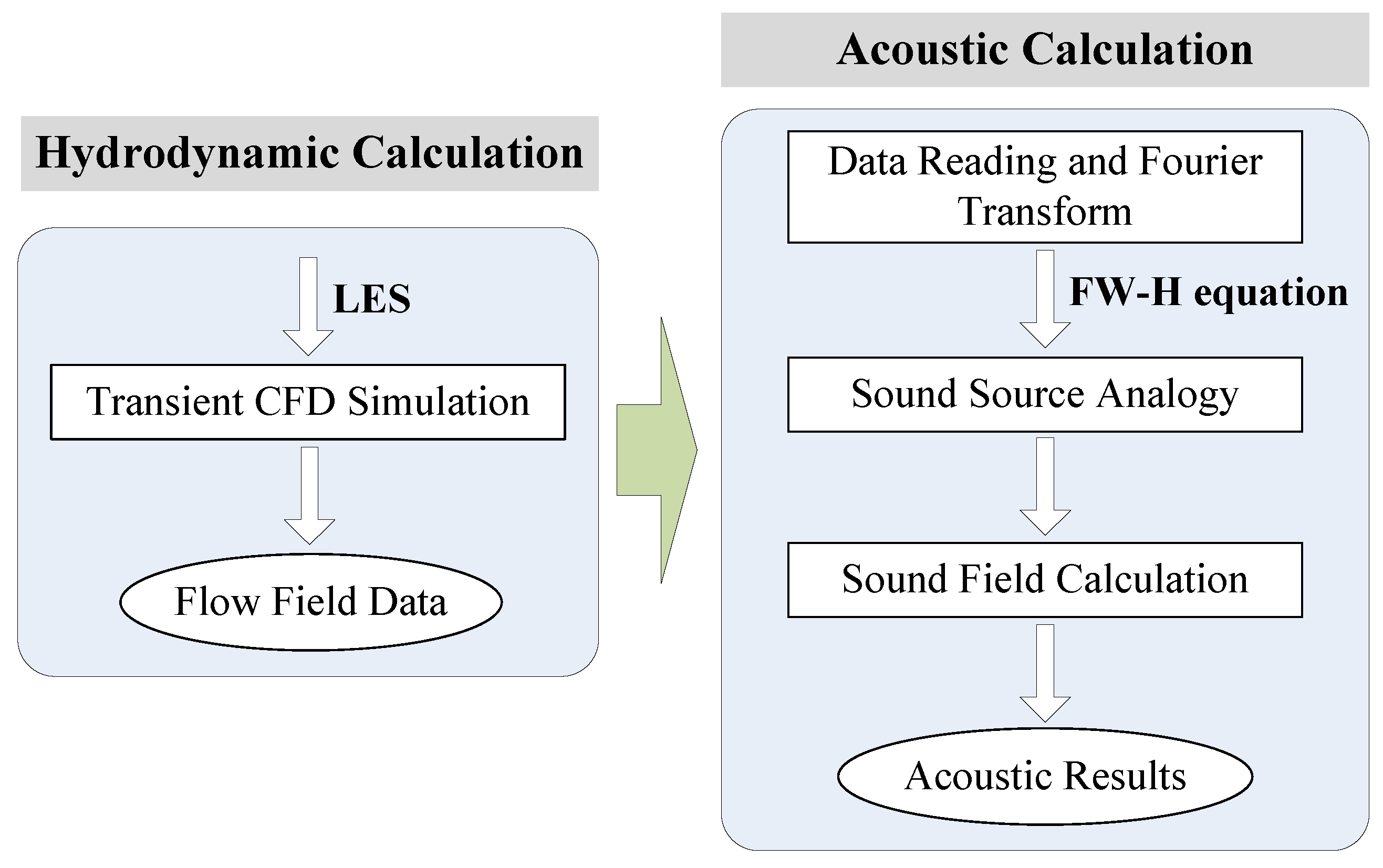
2. Computational Methods

Large eddy simulations (LES) combined with the Ffowcs Williams and Hawkings (FW-H) equation were applied to simulate the hydrodynamic noise of 3D hydrofoil. LES were performed first to calculate the hydrodynamic characteristics of the flow field with a transient Computational Fluid Dynamics (CFD) method [45]. Then, the sound pressure levels were obtained from the fluctuating surface pressure on the hydrofoils based on the FW-H equation [46]. The flowchart of the numerical simulation is given in Figure 2.

2.1. Large Eddy Simulation Model

Turbulence is the three-dimensional unsteady random motion observed in fluids at moderate to high Reynolds numbers [47]. There are three main numerical methods, including direct numerical simulation (DNS), Reynolds-averaged Navier–Stokes (RANS) equation, and LES. The most accurate results could be obtained with DNS. However, in most situations, it is not feasible to resolve the wide range of scales in time and space by using DNS, as the central processing unit (CPU) requirements would by far exceed the available computing power. For this reason, averaging procedures are applied to the Navier–Stokes equations to obtain the flow field characteristics equivalently and rapidly. The most well-known one is the RANS equation, through which a smooth variation of the averaged velocity and pressure fields can be obtained. With low spatial resolution and a small workload, it cannot reflect the fluctuation of the flow field precisely. As a result, LES is proposed to overcome the shortcomings of the other two above methods. It not only greatly reduces the computational complexity, but also obtains the low-frequency evolution information in the instantaneous turbulent flow field with high numerical accuracy. Therefore, this method can simulate the detailed characteristics of the pulsation in the flow field better, so as to calculate the acoustic field more accurately. An incompressible simulation was used for the LES model in this paper.

In the theory of LES, there are two parts for turbulent vortices: the low-pass filtered quantity $\overline{\phi }$, representing large scale vortices before the filter cut-off, and the sub-grid scale quantity $\phi \prime$, representing small-scale vortices after the filter cut-off. The variable $\overline{\phi }$ after filtering is the average in the spatial domain, which is obtained directly by solving the governing equation of LES, while the filtered variable $\overline{\phi }(x)$ is solved by establishing the turbulence model.

$$\overline{\phi }(x)={\displaystyle {\int }_D\phi (x\prime )G(x,x\prime )\mathrm{d}x\prime }$$

(1)

where $D$ is the flow area, $\mathrm{x}\prime$ is the spatial coordinate of the actual flow, $x$ is the large-scale spatial coordinate after filtering, $G(x,x\prime )$ is the filtering function, which can be written as:

$$G(x,x\prime )=\{\begin{array}{c}\frac{1}{V},\hspace{0.17em}\hspace{0.17em}\hspace{0.17em}x\prime \in V\\ 0,\hspace{0.17em}\hspace{0.17em}\hspace{0.17em}\hspace{0.17em}x\prime \notin V\end{array}$$

(2)

where $V$ is the volume of a computational cell. The substitution of the filtering function $G(x,x\prime )$ of Equation (2) into Equation (1) results in:

$$\overline{\phi }(x)=\frac{1}{V}{\displaystyle {\int }_V\phi (x\prime )\mathrm{d}x\prime ,\hspace{0.17em}\hspace{0.17em}\hspace{0.17em}}x\prime \in V.$$

(3)

Then, the governing equations of LES can be obtained by substituting the mass conservation equation and the transient Navier–Stokes equation into Equation (3):

$$\frac{\partial \overline{\rho }}{\partial t}+\frac{\partial }{\partial x_i}(\overline{\rho }{\overline{u}}_i)=0$$

(4)

$$\frac{\partial }{\partial t}(\overline{\rho }{\overline{u}}_i)+\frac{\partial }{\partial x_j}(\overline{\rho }\overline{u_i{u}_j})=-\frac{\partial \overline{p}}{\partial x_i}+\frac{\partial }{\partial x_j}(\mu \frac{\partial {\overline{u}}_i}{\partial x_j})-\frac{\partial {\tau }_{ij}}{\partial x_j}$$

(5)

where ${\tau }_{ij}$ is the term of sub-grid stress, also called the filtered stress tensor, represented as:

$${\tau }_{ij}=\overline{\rho }\left(\overline{u_i{u}_j}-{\overline{u}}_{{}_i}{\overline{u}}_{{}_j}\right).$$

(6)

The sub-grid stress ${\tau }_{ij}$ denotes the momentum transport between small-scale vortex $\phi \prime$ and large-scale vortex $\overline{\phi }$. Additionally, the effect of small-scale fluctuations on the overall flow field is quantified. To make Equation (5) enclosed, the corresponding sub-grid model has to be constructed. At present, the sub-grid model is based largely on the hypothesis proposed by Boussinesq [48], and the sub-grid stress is determined as:

$${\tau }_{ij}-\frac{1}{3}{\tau }_{\mathrm{kk}}{\delta }_{ij}=-2{\mu }_t{\overline{S}}_{ij}$$

(7)

where ${\delta }_{ij}$ is the sub-grid scale of Reynolds stress, ${\mu }_t$ is the coefficient of the sub-grid eddy viscosity, and ${\overline{S}}_{ij}$ is the deformation rate tensor corresponding to the scale of solution, which can be written as:

$${\overline{S}}_{ij}=\frac{1}{2}\left(\frac{\partial {\overline{u}}_i}{\partial x_j}+\frac{\partial {\overline{u}}_j}{\partial x_i}\right).$$

(8)

The eddy viscosity hypothesis above will transform solving the sub-grid stress into solving for the sub-grid scale eddy viscosity coefficient. The Smagorinsky–Lilly model is developed to solve this problem. The coefficient of the sub-grid eddy viscosity, ${\mu }_t$, can be obtained as:

$${\mu }_t=\overline{\rho }{L}_{\mathrm{s}}^2\left|\overline{S}\right|$$

(9)

$$\left|\overline{S}\right|=\sqrt{2{\overline{S}}_{ij}{\overline{S}}_{ij}}$$

(10)

where $L_{\mathrm{s}}$ is the mixing length of sub-grid, and it can be expressed as:

$$L_{\mathrm{s}}=\min (kd,C_s\Delta )$$

(11)

where $k$ is Karman constant, $d$ is the distance from the node to the nearest wall, $C_s$ is Smagorinsky constant, and $\Delta$ is the filter scale.

2.2. Ffowcs-Williams and Hawkings Acoustics Model

In the direct method of predicting hydrodynamically generated noise, both generation and propagation of sound waves are directly computed by solving the appropriate fluid dynamics equations. It is thus computationally expensive and difficult inasmuch as it requires very fine computational meshes, highly accurate numbers all the way to receivers, and acoustically nonreflecting boundary conditions [49], whereas for the methods based on acoustic analogy, such as the FW-H equation, the propagation of sound from its generation is essentially decoupled, allowing one to separate the flow solution process form the acoustic analysis. By solving the FW-H equation, the sound pressure level spectrum and total sound pressure level at the observer points are then calculated from the fluctuating surface pressure on the hydrofoil.

The Lighthill equation is the foundation of hydrodynamic noise, which is derived by the RANS equation and the continuity equation, expressed as:

$$\frac{\partial \rho }{\partial t}+\frac{\partial }{\partial x_i}(\rho u_i)=Q$$

(12)

$$\frac{\partial }{\partial t}(\rho u_i)+\frac{\partial }{\partial x_j}(\rho u_i{u}_j+p{\delta }_{ij}-{\tau }_{ij})=F$$

(13)

where $Q$ is the radiation of unit volume source per unit time and $F$ is the generalized force per unit volume. Subtracting the result of differentiating Equation (12) with respect to time $t$ from the result of differentiating Equation (13) with respect to $x_i$, results in:

$$\frac{{\partial }^2\rho }{\partial t^2}-c_0^2{\nabla }^2\rho =\frac{\partial Q}{\partial t}-\frac{\partial F}{\partial x_i}+\frac{{\partial }^2{T}_{ij}}{\partial x_i\partial x_j}$$

(14)

where $T_{ij}$ is the Lighthill stress tensor, represented as:

$$T_{ij}=\rho u_i{u}_j+{\tau }_{ij}-c_0^2\rho {\delta }_{ij}.$$

(15)

It can be seen from Equation (14) that, if radiation $Q$ changes with time, generalized force $F$ changes with time, or Lighthill stress tensor $T_{ij}$ changes, hydrodynamic noise will be produced.

For solid wall turbulence, the general solution for Equation (14) can be written as:

$$\rho (\tilde{x},t)-{\rho }_0=\frac{1}{4\pi c^2}\frac{{\partial }^2}{\partial x_i\partial x_j}{\displaystyle {\int }_V\frac{T_{ij}\left(\tilde{y},t-\frac{r}{c}\right)}{r}}\mathrm{d}V(\tilde{y})-\frac{1}{4\pi c^2}\frac{\partial }{\partial x_i}{\displaystyle {\int }_V\frac{P_i\left(\tilde{y},t-\frac{r}{c}\right)}{r}}\mathrm{d}V(\tilde{y})$$

(16)

$$P_i=-l_j{p}_i{}_j$$

(17)

where $l_j$ is cosine in the normal direction of source plane area $S$ and the direction is from inside to outside for the boundary-layer flow of a flat plate, $l_1=l_3=0$, $l_2=1$. In this way, $P_1=-{\sigma }_{12}$, $P_2=p$, and $P_3=-{\sigma }_{32}$, where ${\sigma }_{12}$ and ${\sigma }_{32}$ represent the shear stress $p_{12}$ and $p_{32}$, separately. Substituting the value of $P_i$ into Equation (16) yields the following sound pressure equation:

$$\rho (\tilde{x},t)=\frac{1}{4\pi }\frac{{\partial }^2}{\partial x_i\partial x_j}{\displaystyle {\int }_{2V}\frac{T_{ij}}{r}}\mathrm{d}V(\tilde{y})-\frac{1}{2\pi }\frac{\partial }{\partial x_1}{\displaystyle {\int }_S\frac{{\sigma }_{12}}{r}}\mathrm{d}S(\tilde{y})-\frac{1}{2\pi }\frac{\partial }{\partial x_3}{\displaystyle {\int }_S\frac{{\sigma }_{32}}{r}}\mathrm{d}S(\tilde{y}).$$

(18)

Then, a further transformation is conducted into a form suitable for engineering calculation of hydrodynamic sound pressure:

$$\rho (\tilde{x},t)=\frac{1}{4\pi c^2}\frac{x_i{x}_j}{r^3}{\displaystyle {\int }_{2V}\frac{{\partial }^2{T}_{ij}}{\partial t^2}}\mathrm{d}V(\tilde{y})+\frac{1}{2\pi c}\frac{x}{r^2}{\displaystyle {\int }_S\frac{\partial {\sigma }_{12}}{\partial t}}\mathrm{d}S(\tilde{y})+\frac{1}{2\pi c}\frac{z}{r^2}{\displaystyle {\int }_S\frac{\partial {\sigma }_{32}}{\partial t}}\mathrm{d}S(\tilde{y}).$$

(19)

From Equation (18), it can be seen that the hydrodynamic noise is composed of monopole, dipole, and quadrupole sound sources. Then, the sound pressure in the time domain is obtained. After Fourier transformation, the noise characteristics in the frequency domain are calculated. The sound pressure level (SPL) is defined as

$$\mathrm{SPL}\left(\mathrm{dB}\right)=20{\log }_{10}\left(\frac{p}{p_{ref}}\right)$$

(20)

where $p$ is the acoustic pressure and $p_{ref}$ is the reference acoustic pressure. For sound transmission in water, the reference pressure is defined as 1 $\mathsf{\mu }\mathrm{Pa}$($1\times {10}^{-6}\mathrm{Pa}$). Correspondingly, the overall sound pressure level (OASPL) is obtained as

$$\mathrm{OASPL}\left(\mathrm{dB}\right)=10{\log }_{10}\left({\displaystyle \sum _{i=1}^n{10}^{\frac{\mathrm{SPL}(i)}{10}}}\right)$$

(21)

where $\mathrm{SPL}(i)$ is the octave band sound pressure level in the broadband frequency domain and $n$ is the number of octave bands from the lowest frequency to the highest frequency concerned.

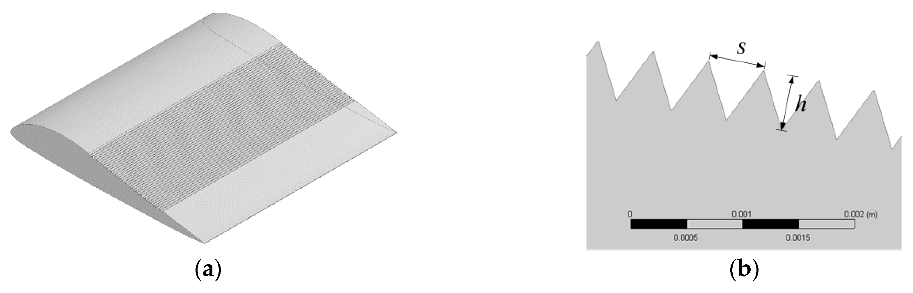
3. Design of Spanwise Microgrooves on the Surface of Hydrofoils

The airfoil shapes used in this paper are created from the FF-77-W airfoil shape, which is available at [50]. As is shown in Figure 3, the relative thickness of the airfoil is 14.8% of the length of the chord. When the fluid flows around the hydrofoil, it will produce drag in the flow direction and lift in the vertical direction. Boundary layer separation occurs when the flow angle is larger than a certain value. The location of the separation point and the flow pattern in the boundary layer are closely related to the surface structure of the airfoil, and they also determine the resistance of the airfoil. The turbulent boundary layer has stronger fluid mixing, more uniform fluid kinetic energy distribution, and smaller shape resistance compared with that of laminar boundary layer. Therefore, increasing the surface roughness of the structure is often an effective measure to improve the flow field.

According to the results of Walsh [51,52,53], the optimal drag reduction effect could be obtained with microgrooves when its non-dimensional height $h^{+}$ and non-dimensional spacing $s^{+}$ are both 15. The expression of $h^{+}$ and $s^{+}$, according to Walsh, are defined as

$$h^{+}=\frac{h{u}_{\infty }}{v}\sqrt{\frac{c_f}{2}}$$

(22)

$$s^{+}=\frac{s{u}_{\infty }}{v}\sqrt{\frac{c_f}{2}}$$

(23)

where $h$ is the microgroove height, $s$ is the microgroove spacing, $v$ is the kinematic viscosity, $u_{\infty }$ is the free-stream velocity, and $c_f$ is the local skin friction coefficient. In this way, the dimension parameters of the microgrooves are determined. As a preliminary design inspired by [43] and [44], partial coverage is applied to the upper surface from 40% of the airfoil chord to 80% of the airfoil chord. The overall 3D hydrofoil partially covered by microgrooves and details of the microgrooves are shown in Figure 4.

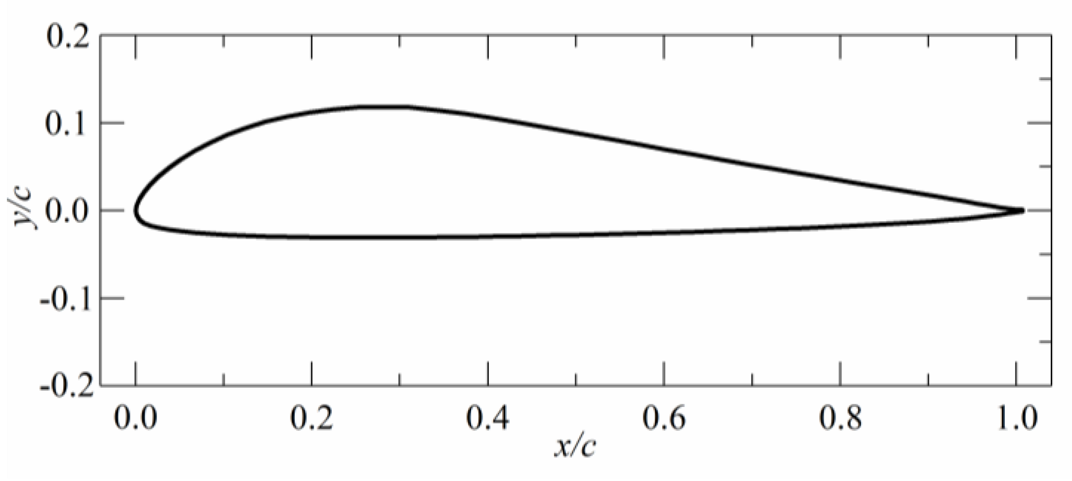
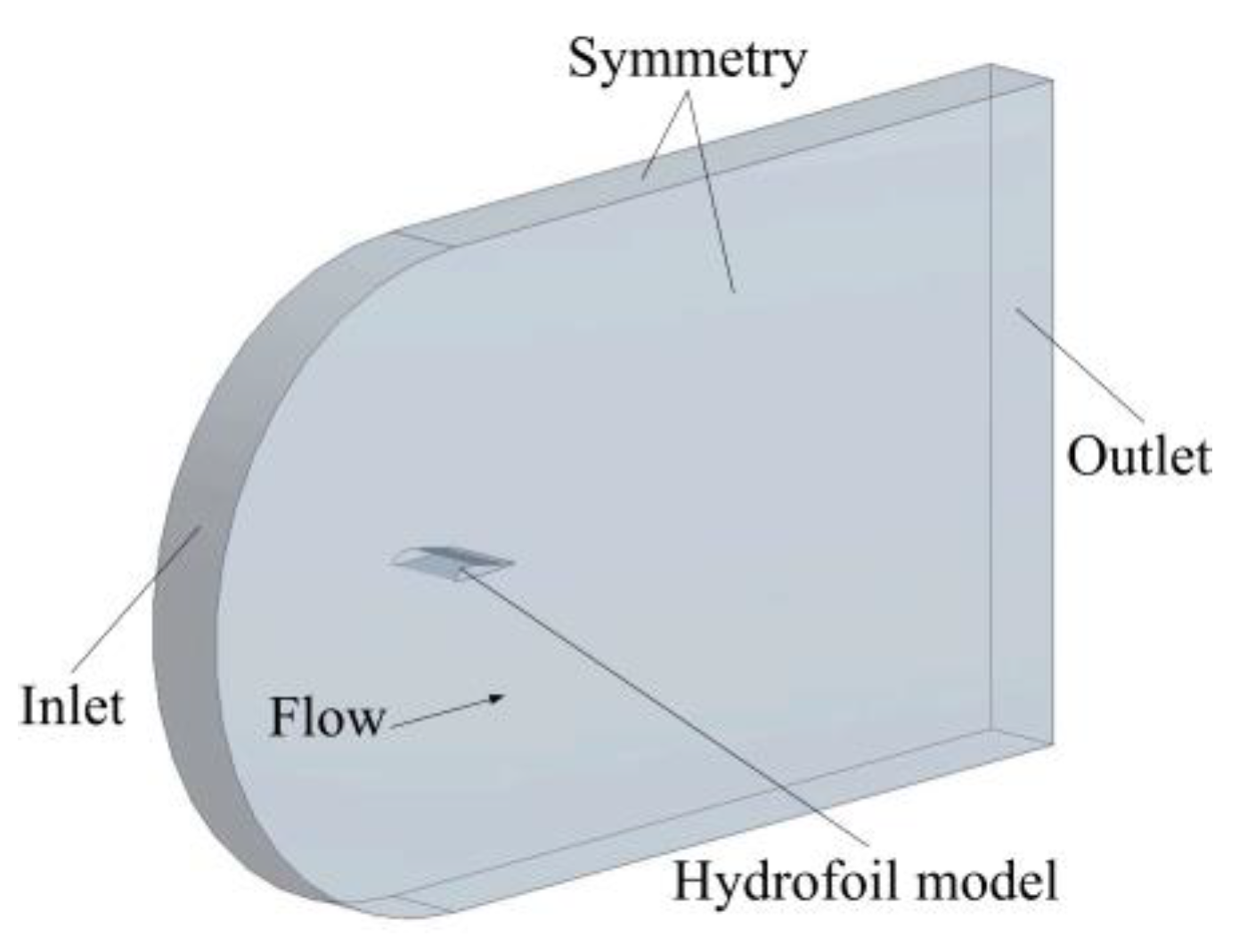
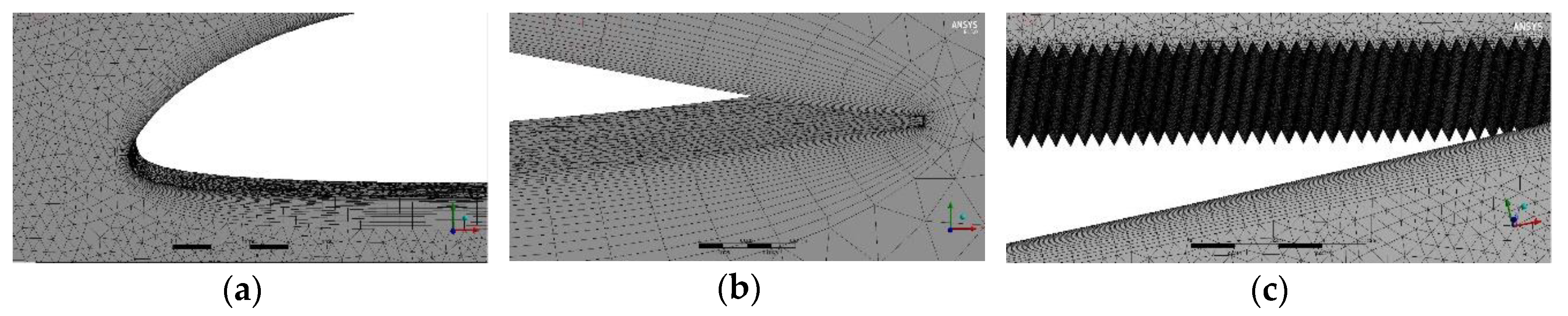
4. Computational Model

The transient simulations were performed utilizing the FLUENT code in the ANSYS v15.0 environment. In the simulation, the computational domain was sized to decrease the blockage effect and to allow for full development of the upstream flow. The hydrofoil, with a fixed chord $c$, stood in the middle position of the vertical direction of the computational domain. The upstream inlet was $5c$ from the leading edge of the hydrofoil, and the outlet boundary was placed $10c$ downstream of the trailing edge of the hydrofoil. Spanwise length in the $z$-direction was set to 50 mm (0.99c). The computational domain and the corresponding boundary conditions are shown in Figure 5.

Due to the small dimensions of microgrooves (less than 1 mm), unstructured grids were applied in the computational domain. In order to make the calculation results more accurate, (1) mesh refinement was carried out at the microgrooves, and (2) boundary layer mesh was applied at the surface of the hydrofoil with more layers in the boundary layers and fine element size of the boundary layers. The details of the grids near the leading edge region, the trailing edge region, and the microgrooves are shown in Figure 6.

A flow with uniform and steady velocity of 1 m/s was applied at the inlet of the computational domain, and a pressure outlet boundary was imposed at the outlet of the computational domain. A no-slip boundary condition was applied at the surface of the hydrofoils. To improve the reliability of the numerical model, symmetry boundary conditions were used at the four side walls of the domain, which allowed us to consider the computational domain in a larger domain, avoiding the effects of walls.

5. Numerical Method Verification and Validation

Because there is no available experimental data about the hydrofoils studied in this paper, airfoil NACA0012 was selected to test the reliability and accuracy of the present numerical model. The verification and validation of the present numerical method were as follows. The Reynolds numbers of the NACA0012 airfoil were 1.0 × 10⁵ for grid independence verification and acoustical validation and 2.88 × 10⁶ for the flow field validation. The transient pressure-based solver was adopted with the drop of all scaled residuals below 1.0 × 10⁻⁵, which was employed as the convergence criterion. The time step size was 2.0 × 10⁻⁵, and the maximum number of iterations was set as 5.0 × 10⁴, which enabled the sound frequency range calculated to be 1 Hz~20 kHz with an interval of about 1 Hz. The non-iterative time-advancement scheme, which significantly speeds up transient simulations by performing only a single outer iteration per time step, was applied in the simulation. The fractional-step method was adopted in ANSYS FLUENT as a velocity-coupling scheme in a non-iterative time-advancement algorithm for the solution method in this paper.

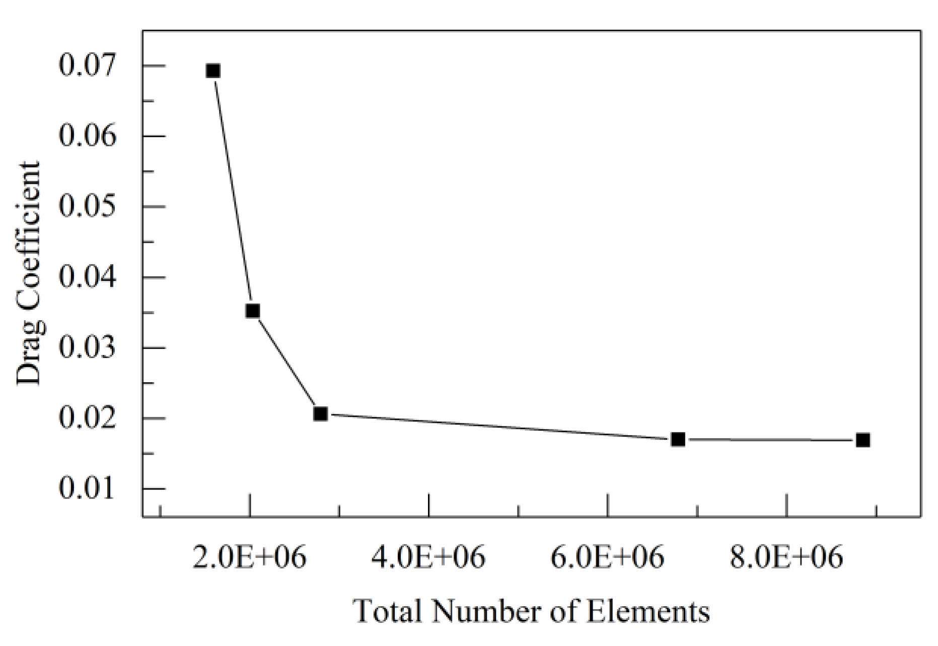
5.1. Verification

A grid resolution study was performed to evaluate the influence of grid resolution on the drag coefficient of five different meshing schemes. The angle of attack of the airfoil was zero. The details of the five mesh schemes, including the total number of elements, the parameters of boundary layers, and the element size along the spanwise direction are listed in

Table 1. Mesh details of the selected meshing schemes for mesh independence study.

Details of Mesh	Mesh 1	Mesh 2	Mesh 3	Mesh 4	Mesh 5
Total number of elements	1,593,064	2,035,810	2,793,386	6,788,150	8,856,372
Layer number of boundary layers	10	20	10	20	30
Element size of boundary layers (m)	8.0 × 10−4	8.0 × 10−4	5.0 × 10−4	5.0 × 10−4	5.0 × 10−4
Element size along spanwise direction	2.0 × 10−3	2.0 × 10−3	2.0 × 10−3	1.0 × 10−3	1.0 × 10−3

. The drag coefficient at the angle of attack of zero is calculated by

$$C_d=\frac{F_d}{0.5\rho u_{\infty }^{2}cl}$$

(24)

where $F_d$ is the drag force and $l$ is the spanwise length of the hydrofoil.

Figure 7 presents the results with different grid resolutions. It can be seen that the drag coefficient approximately approached a stable value with the increase of total number of elements. This indicates that further increasing the grid resolution would not significantly affect the results of drag coefficient in the simulation. Considering the economy of time in the simulation, the grid configuration of Mesh 4 was chosen for the following simulations.

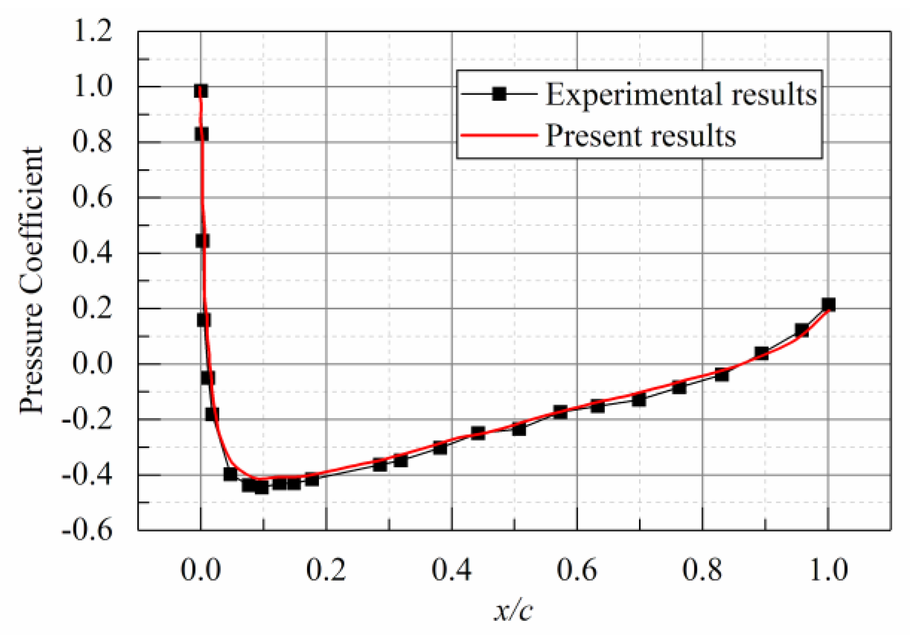
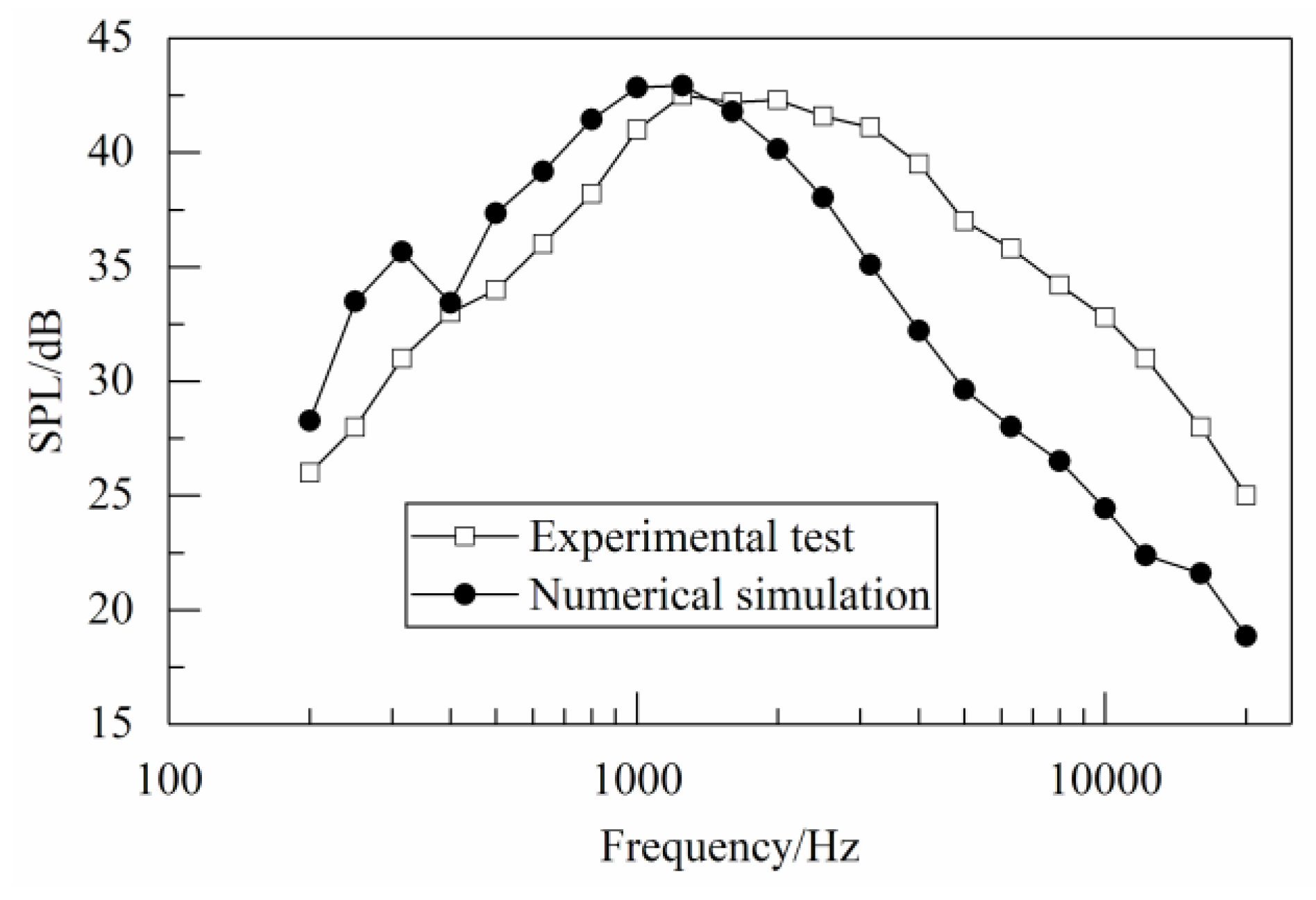
5.2. Validation

In order to validate the accuracy of the numerical method used in this paper, the flow field characteristics and sound field performance were evaluated with the experimental results simultaneously.

First, the surface pressure coefficients’ distribution on the NACA0012 airfoil with an angle of attack at 0° was compared with the experiment results [54], as shown in Figure 8. In the simulation, the Reynolds number was 2.88 × 10⁶, which was in accordance with the experimental test. It was shown that the numerical results have fairly good agreement with the experimental results tested in the wind tunnel.

Then, the predictive SPL by experimental test for the NACA0012 airfoil at the observing point was used to verify the accuracy of the acoustic signals. The observing point was perpendicular to and 1.22 m from the trailing edge and the model midspan. In the validation, the model of smooth surface airfoil where the boundary layers were untripped was chosen, the inlet flow velocity was 31.7m/s, and the angle of attack was 0°. Figure 9 shows the comparison of SPL in 1/3 octave frequency bands of 30.48-cm-chord NACA0012 airfoil in the experimental test [6] and the numerical simulation. It can be observed that the numerical results are in close agreement with the experimental results at low and medium frequencies, while for the high-frequency range, the trend was consistent. Considering that the most concern was concentrated on the main peaks of the noise spectrum at lower frequency in the subsequent analysis, which dominated the main noise energy, a conclusion could be drawn that the numerical method applied in this paper is able to study the noise reduction of biomimetic hydrofoil.

6. Results and Discussions

The numerical calculations of the hydrofoil were conducted at an angle of attack of 0° and a Reynolds number of 5.0 × 10⁴, based on using the hydrofoil chord as the characteristic length. The hydrofoil was created from the FF-77-W airfoil shape, whose relative thickness was 14.8% of the length of the chord, as mentioned in Section 3. The dimensions of the computational domain are shown in Section 4. A similar density grid (Mesh 4), as shown in Section 5.1, was adopted to calculate both the flow field characteristics and sound field performance of the original hydrofoil model and the biomimetic hydrofoil model. To complete the numerical calculation, the relevant material properties of water used in this paper are listed in

Table 2. Material properties of water used in the simulation.

Description	Parameter and Value
Temperature	$T$ = 20 °C
Density	$\rho$ = 998.2 kg/m3
Viscosity	$\mu$ = 0.001003 kg/(m·s)
Sound speed	$v$ = 1483 m/s
Reference acoustic pressure	$p_{ref}$ = 1.0 × 10−6 Pa

.

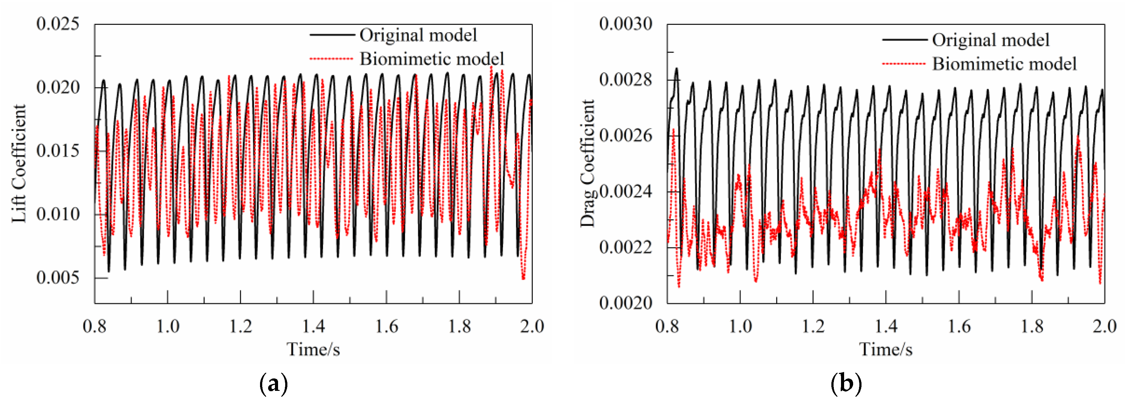
6.1. Analysis of Hydrodynamic Performance

Figure 10 shows time histories of the hydrodynamic force coefficients of the original hydrofoil and biomimetic hydrofoil at 0.8–2.0 s, with a running average over 5 times of calculation. It can be seen that the curves of the lift coefficient and drag coefficient for the original hydrofoil fluctuated periodically. Further, it can be easily seen that there was a small pulse near the peak of each period of drag coefficient, which was largely due to the instability of the flow velocity gradient, while the for biomimetic model, there was not an evident periodicity of properties for the lift coefficient curve, but the values of the lift coefficient were very close. The drag coefficient curve for the biomimetic model was even much more arbitrary than the lift coefficient curve. Moreover, it is shown in Figure 10 that the lift coefficient of the biomimetic model was almost unchanged, and the drag coefficient of the biomimetic model was slightly decreased. In total, the amplitudes of fluctuations with variation of time were significantly lower than that of the original hydrofoil.

In addition, the sound pressure with variation of time of the original hydrofoil at three different observing points was depicted in Figure 11. The three points, named Receiver 1, Receiver 2, and Receiver 3, were perpendicular to the trailing edge and 0.1 c, 0.3 c, and 5.5 c from the model midspan, respectively. From Figure 11, it can be seen that the amplitudes of the sound waves gradually decreased with the sound transmission with distance. Further, one can observe that the period of the three curves was the same.

6.2. Analysis of Near-Field Hydrodynamic Noise

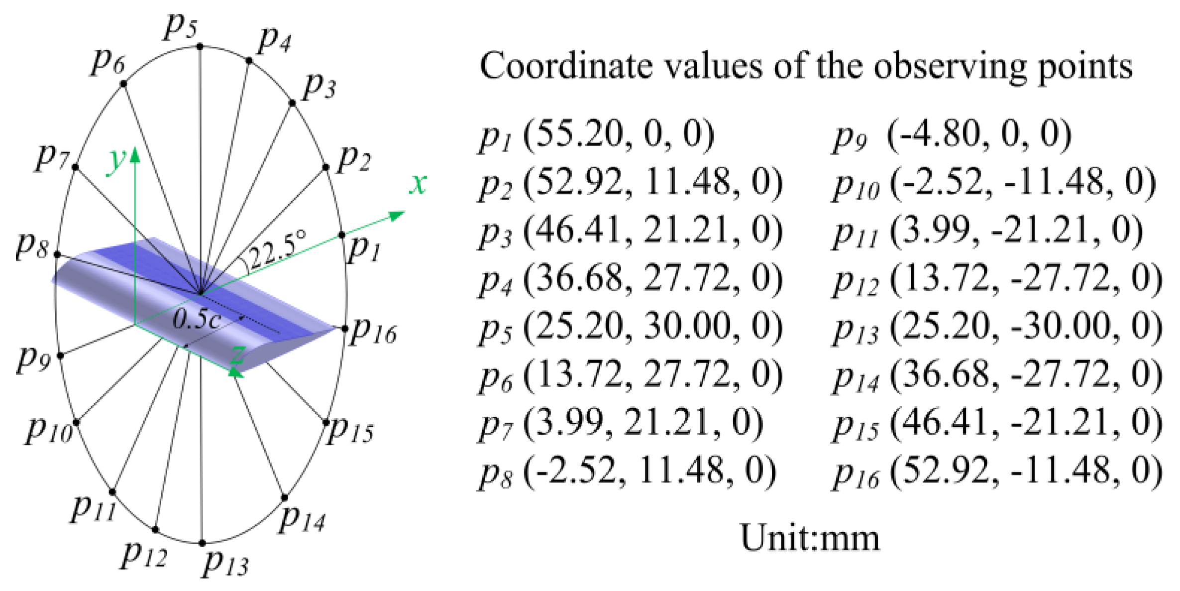
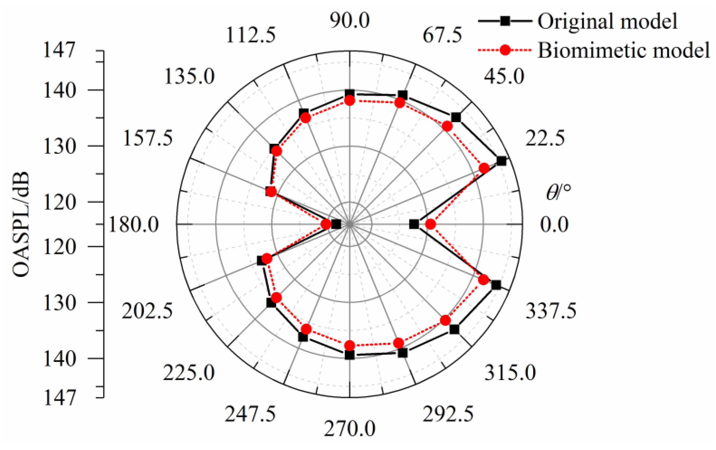
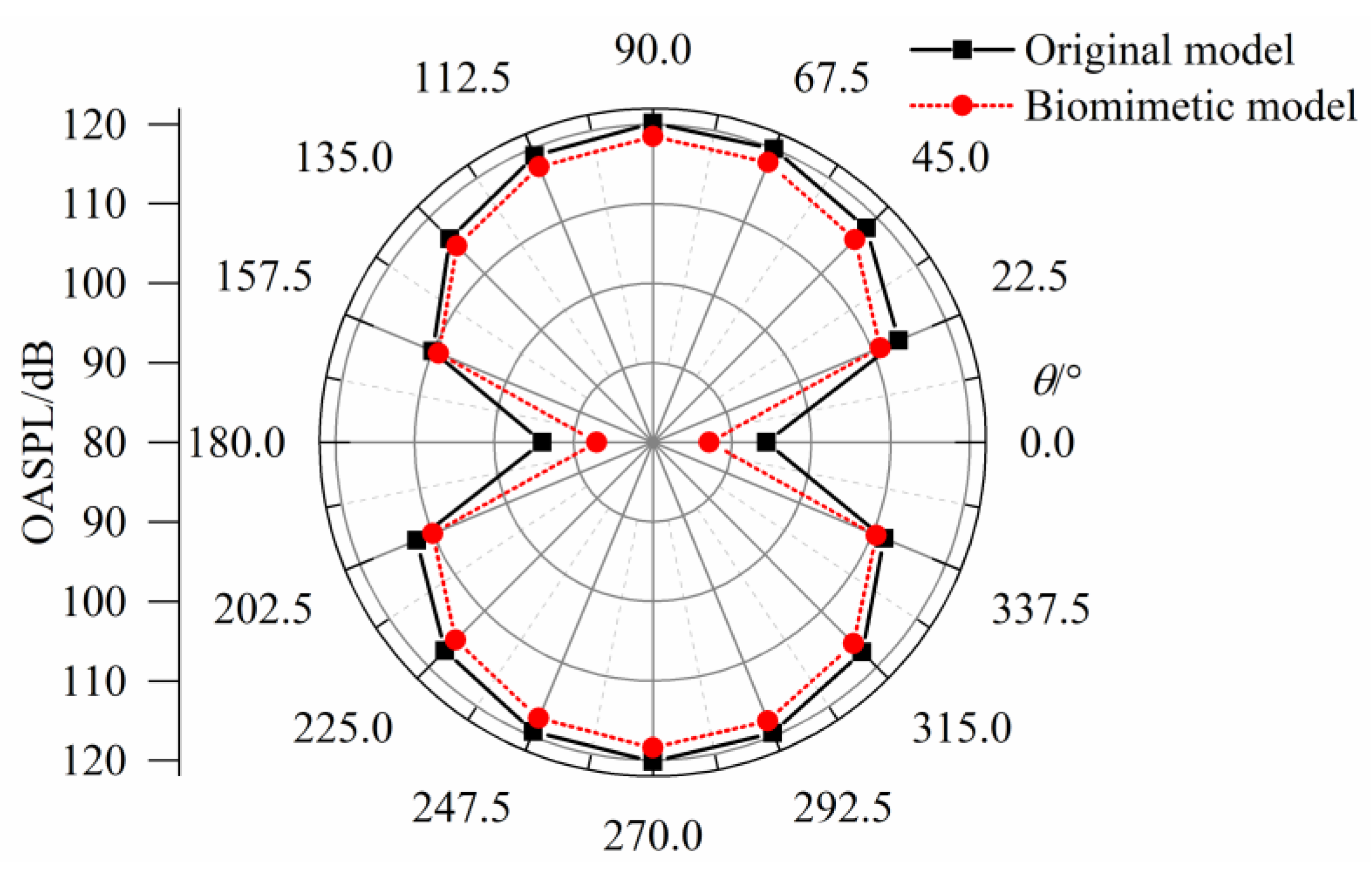
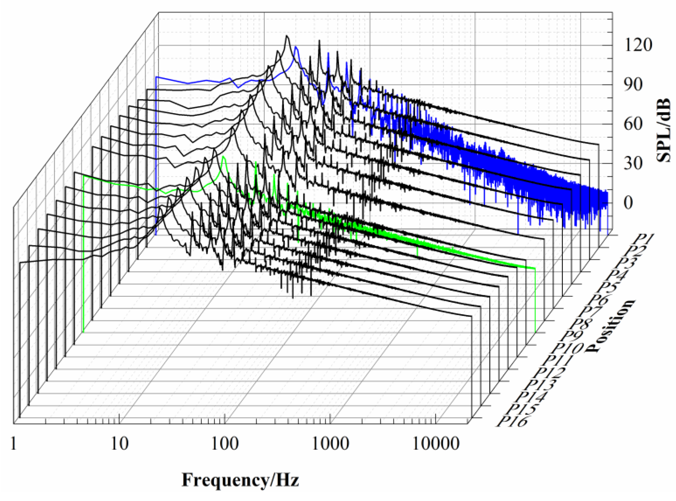
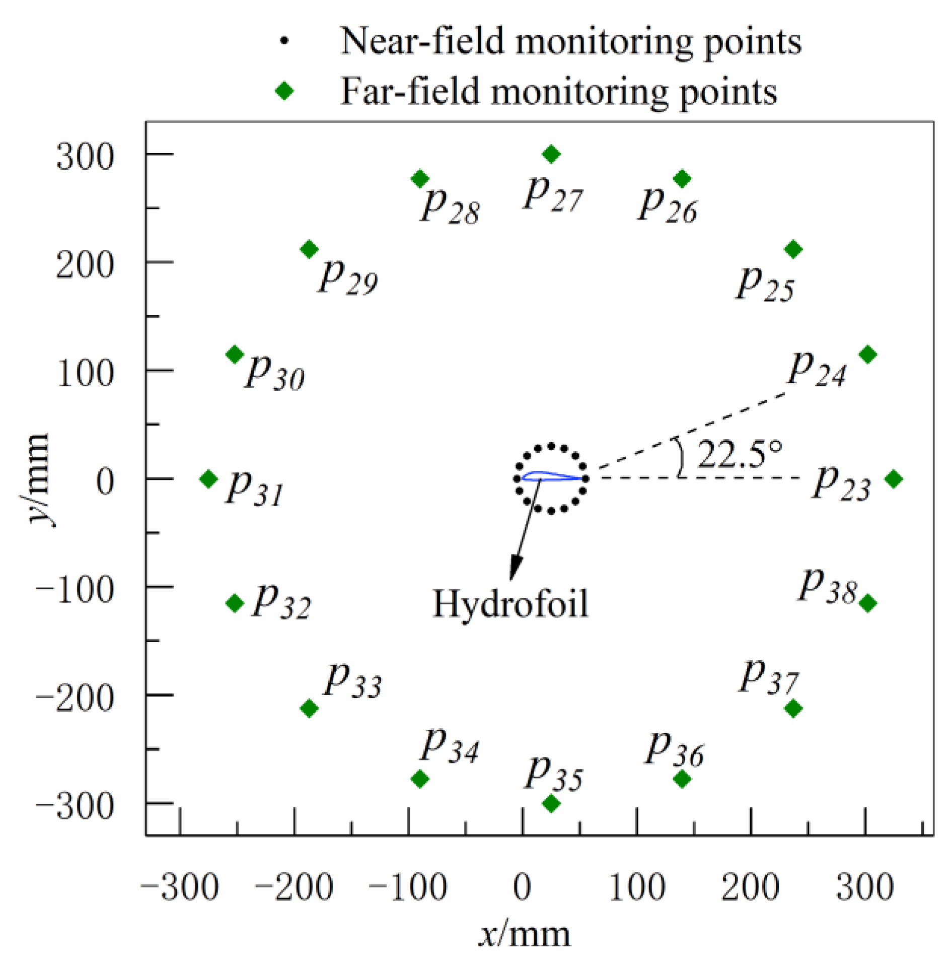
6.2.1. Noise Characteristics along the Circumferential Direction

A total of 16 observing points were defined to evaluate the acoustic performance of near-field hydrofoil noise along the circumferential direction, which are presented in Figure 12. It can be seen that the observing points were evenly distributed in a circle with a radius of 30.00 mm. As is shown in Figure 12, the origin of the coordinate was at the midspan of the leading edge, and the center of the circle was obtained by translating the origin of the coordinate along the x-axis direction. The predicted SPL for each observing point of original hydrofoil as a function of frequency is shown in Figure 13. It can be seen that all of the curves exhibited similar peaks and dips and followed the same trend, which first increased in the lower frequency range and then decreased in the higher frequency range, except for the points near the trailing edge p₁ and leading edge p₉. To show the noise characteristics of the original hydrofoil and biomimetic models, four representative observing points were chosen, that is, p₁, p₅, p₉, and p₁₃. The comparisons of the predicted SPL spectra generated from the original and biomimetic model for the four observing points are illustrated in Figure 14. Additionally, the OASPL of the 16 observing points for the two models are presented in Figure 15.

It can be observed from Figure 14 that the noise spectra generated from the original hydrofoil and biomimetic hydrofoil were totally different in these four observing points. The SPL generated from biomimetic model increased at low frequencies, and the frequency of the main peaks of the SPL curve all increased a little. As for the noise spectrum at higher frequency, it can obviously be seen that the biomimetic model would generate more noise than the original hydrofoil at observing point p₁. Combined with the results of Figure 15, it was shown that the OASPLs of the biomimetic hydrofoil at observing points p₁ and p₉ were larger than those of the original model. Except for observing points p₁ and p₉, all the other observing points had positive effects on noise attenuation. The maximal noise reduction effect was found at observing point p₂, with an overall noise reduction of 3.37 dB.

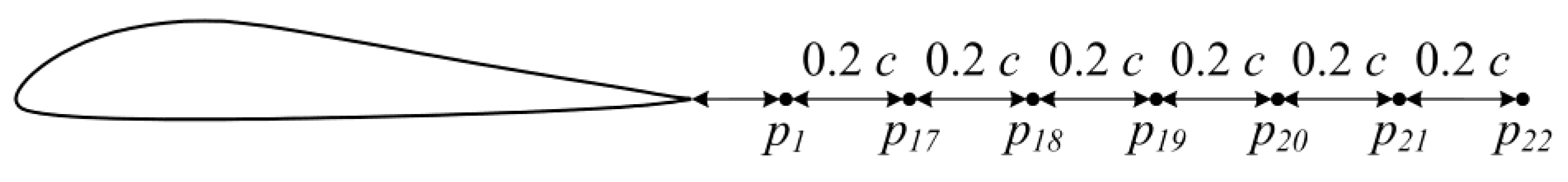
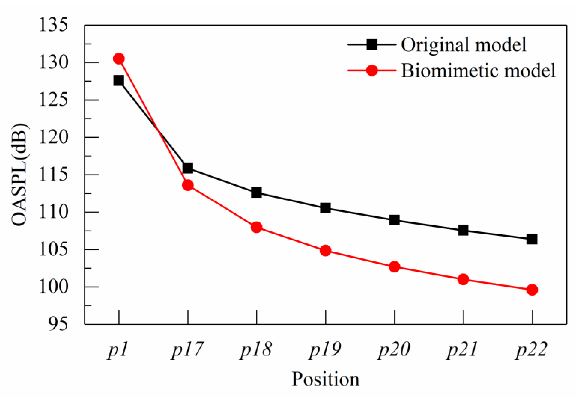
6.2.2. Noise Characteristics along the Radial Direction

Due to the high change rate of sound pressure in the near sound field, which can be found in Figure 11, the noise characteristics along the radial direction were investigated. Another six observing points were chosen, named p₁₇, p₁₈, p₁₉, p₂₀, p₂₁, and p₂₂, as shown in Figure 16. The interval between the neighboring observing points was 0.2 c. Correspondingly, the predicted SPL spectra and predicted OASPLs of the original hydrofoil and biomimetic hydrofoil at the six observing points are shown in Figure 17; Figure 18, respectively.

It can be seen from Figure 17 that the main peaks in the SPL curve gradually faded away in the biomimetic design with the increase of observing distance. Further, the noise reduction effect in the high-frequency range gradually became more intense. As is shown in Figure 18, the overall noise reduction for the six observing points was 2.27 dB, 4.65 dB, 5.67 dB, 6.23 dB, 6.56 dB, and 6.78 dB, respectively. The six observing points had increasingly positive noise reduction effects, which was different from that of observing point p₁.

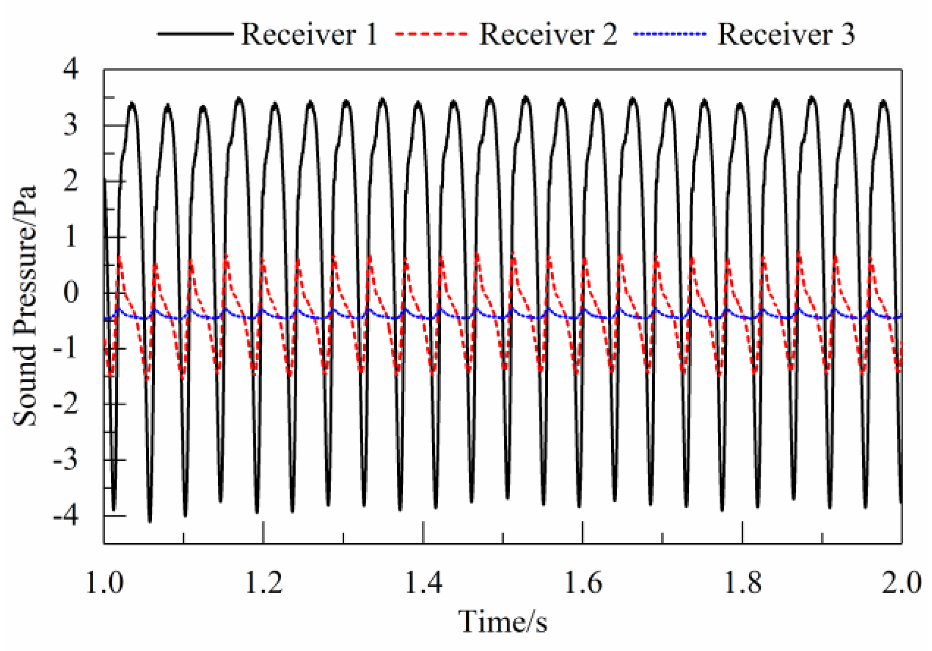
6.3. Analysis of Far-Field Hydrodynamic Noise

To quantify the noise reduction of the biomimetic hydrofoil in the far sound field, another 16 observing points were chosen. As is shown in Figure 19, the observing points were evenly distributed in a circle with a radius of 300.00 mm. In order to observe the comparisons of the two models clearly, the observing points at 0°, 90°, 180°, and 270° were chosen, which was similar to the conduction of the near sound field in Section 6.2.1. The comparisons of the predicted SPL spectra generated from the original hydrofoil and biomimetic models are shown in Figure 20. And the OASPLs of all the far sound field observing points are demonstrated in Figure 21.

It is easily observed from Figure 20 that the main peaks of the original model were eliminated after carrying out biomimetic design. Combined with the result of Figure 21, it can be seen that all of the observing points have achieved a certain degree of noise reduction effect. It is worth noting that the observing points at 0° and 180°, where negative effects could be found in the near sound field, had significant noise reduction effects in the far sound field. Among all of the 16 observing points, the maximal noise reduction was 7.28 dB, obtained at observing point p₂₃.

6.4. Noise Reduction Mechanism

The hydrofoil self-noise is produced by the interaction between the structure and the turbulence produced in its own boundary layer and the near wake [6]. To give a clear view of the flow field, the two-dimensional contours of the flow field at the mid plane of the hydrofoil at 2.0 s are given in this section.

The comparison of the pressure contours between the original hydrofoil and biomimetic hydrofoil is shown in Figure 22. It can be seen that the pressure of the biomimetic model was much more stable than the original one, especially near the region of suction surface. Moreover, the contours of velocities in the y direction and in the flow direction at the trailing edge of the two models investigated in this paper are illustrated in Figure 23; Figure 24, respectively. It is noticeable that the velocity fluctuations in both the y direction and in the flow direction at the trailing edge improved a lot after adding spanwise microgrooved surfaces. The velocity gradient of the flow in the wake of the trailing edge was significantly decreased. To give more explanations for the mechanism of the noise reduction demonstrated in this paper, the streamlines in the groove are exhibited in Figure 25.

As is shown in Figure 25, two pairs of vortices rotating reversely existed in the interior of the microgrooves. It is noticeable that the rotation direction of the larger vortex near the surface of the hydrofoil was favorable to the flow of the external flow field. The “micro-air bearing” introduced by Pan [55] could provide explanations for this phenomenon in this paper. The advantages of surfaces with spanwise microgrooves for retarding the development of the turbulent boundary layer include the following: (1) weakening of the streamwise vortices that spawn the secondary vortices and (2) retention of low-speed fluid within the grooves. For the present cases, the spanwise microgrooves, which were introduced onto the surface of the hydrofoils, consumed the energy of the flow. The existence of these secondary flow vortices plays a similar role to “roller bearings”. These secondary flow vortices are stable in the groove and will not appear on the surface, which would lead to the phenomenon of vortices scattering. In short, the basic idea of underwater noise reduction of hydrofoils with spanwise microgrooved surface is to hinder the process of turbulence, reduce the flow energy, and weaken the intensity of turbulent burst.

7. Conclusions

A biomimetic hydrofoil is proposed in this study with spanwise microgrooved surfaces inspired by sharkskin on the FF-77-W airfoil profile. Firstly, LES were carried out to simulate hydrodynamic characteristics of the hydrofoil; then, the sound pressure at the observing points was calculated based on the FW-H equation. After verifying and validating the numerical method, the hydrodynamic performance and the sound field characteristics were compared between the biomimetic hydrofoil and the original hydrofoil. The main conclusions of this research were as follows:

• The change of the lift coefficient and drag coefficient had no obvious cycle. Compared with the characteristics of original hydrofoil, the lift coefficient of the biomimetic model was almost unchanged, and the drag coefficient of the biomimetic model was slightly decreased.
• In near sound field, the OASPLs of the observing points in the 0° and 180° direction of the biomimetic hydrofoil were larger than those of the original model. With the increase of observing distance along the direction, the OASPL of the biomimetic model gradually became lower than that of original model at the same observing positions. In particular, the maximum noise reduction of 7.28 dB could be obtained at the observing point in the 0° direction of the far sound field, which was the optimal position of all the 16 observing points along the circumferential direction.
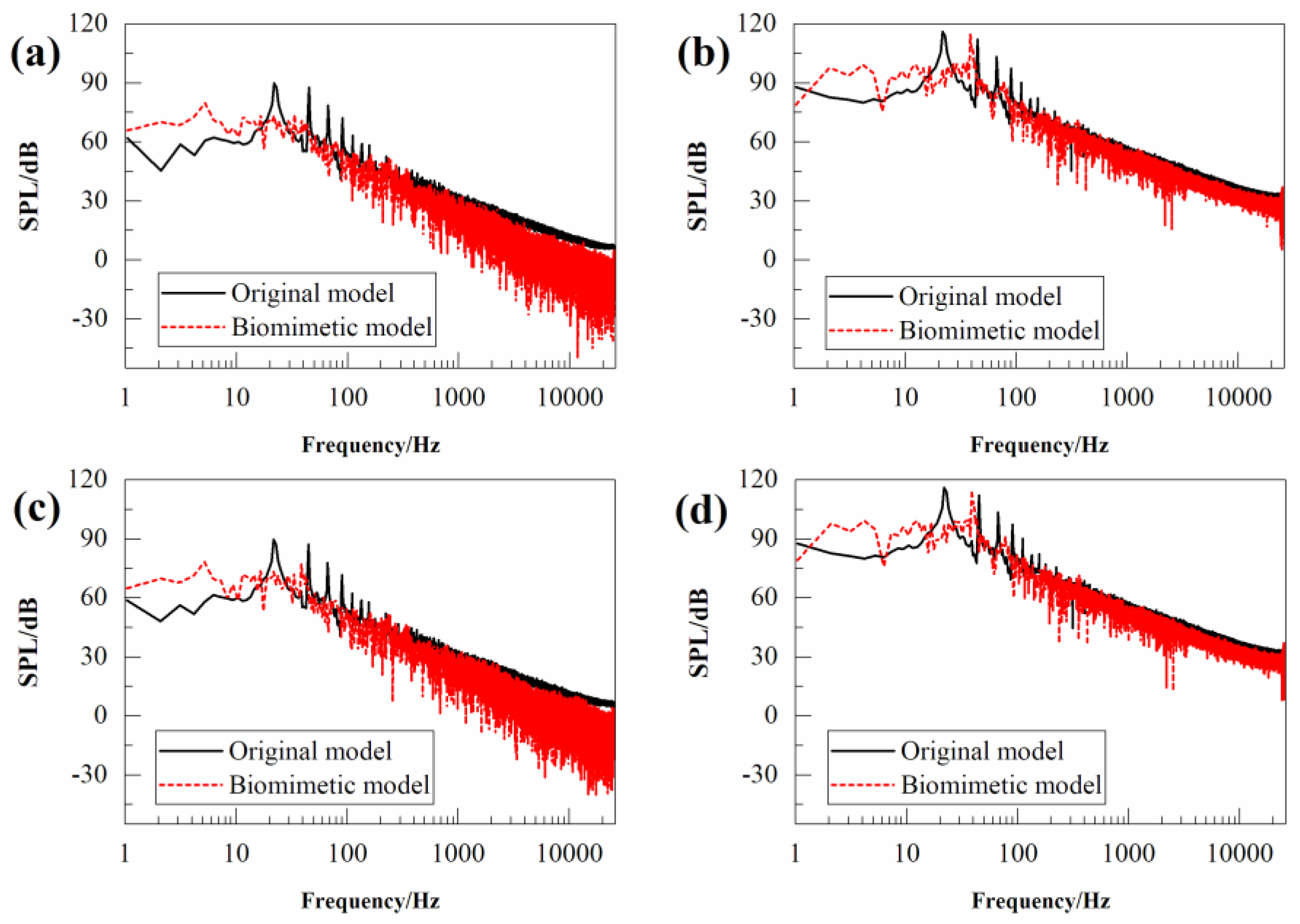
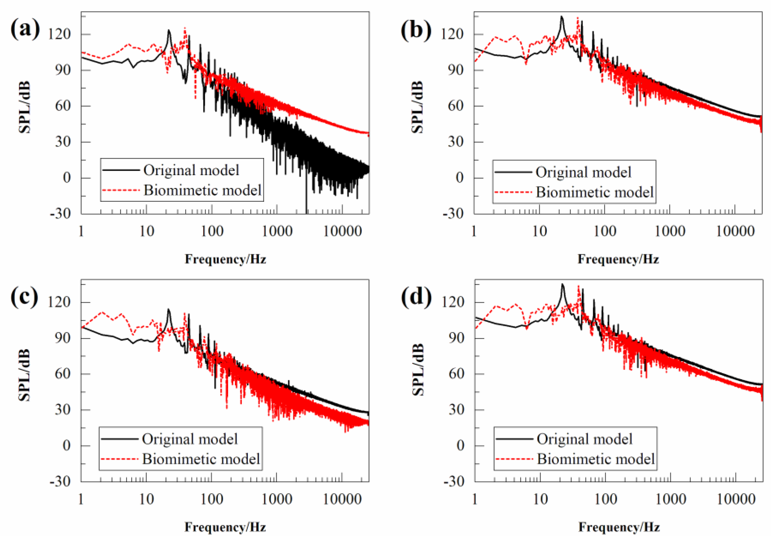
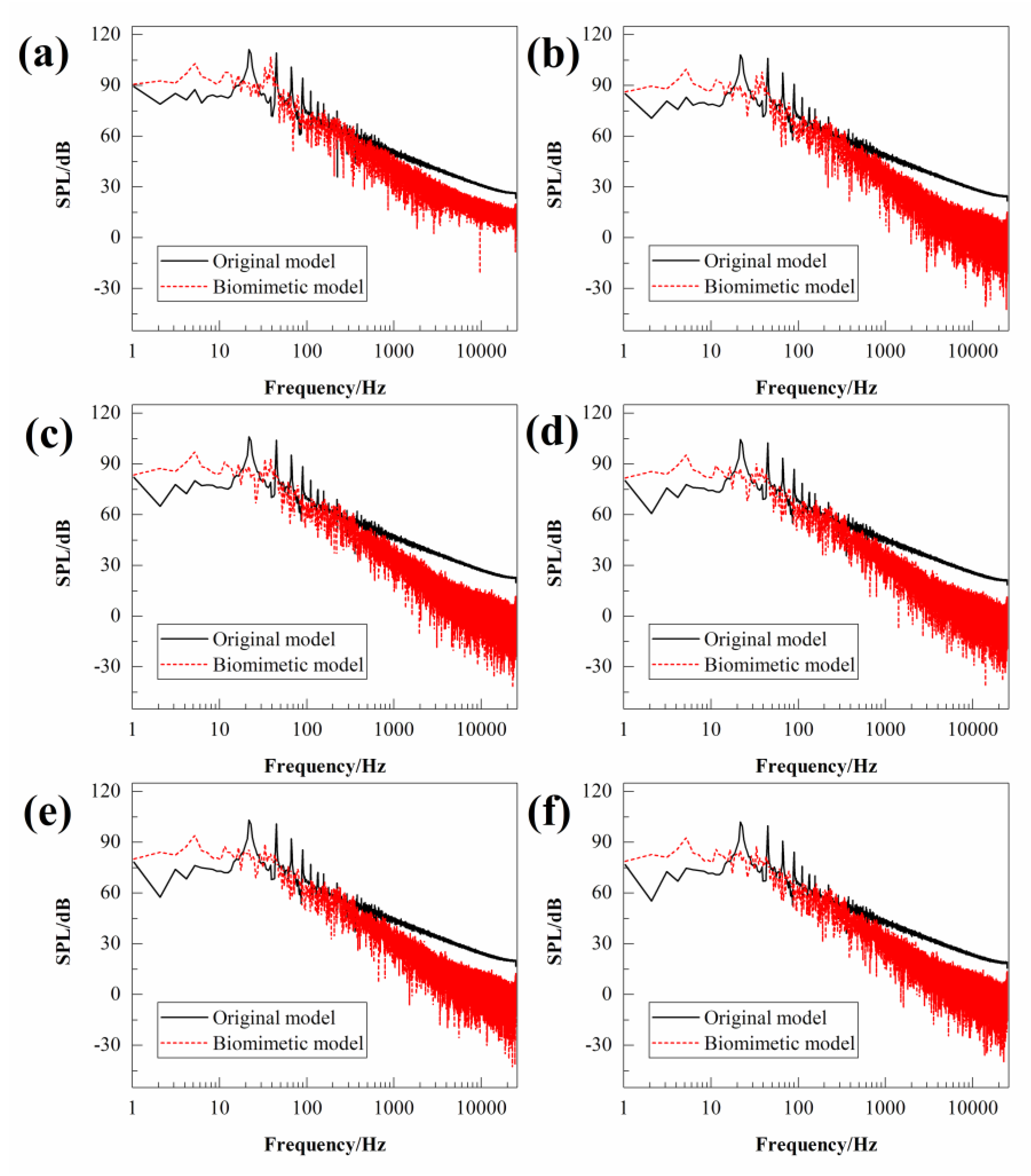
• Compared with the noise spectra of the biomimetic hydrofoil and the original hydrofoil, it can be seen that the SPL of the biomimetic model is higher at low frequencies. In the near sound field, the main peaks in the noise spectrum shifted to a higher frequency, while in the far sound field, it was observed that the main peaks in the noise spectrum almost disappeared, which resulted in a favorable noise reduction effect.
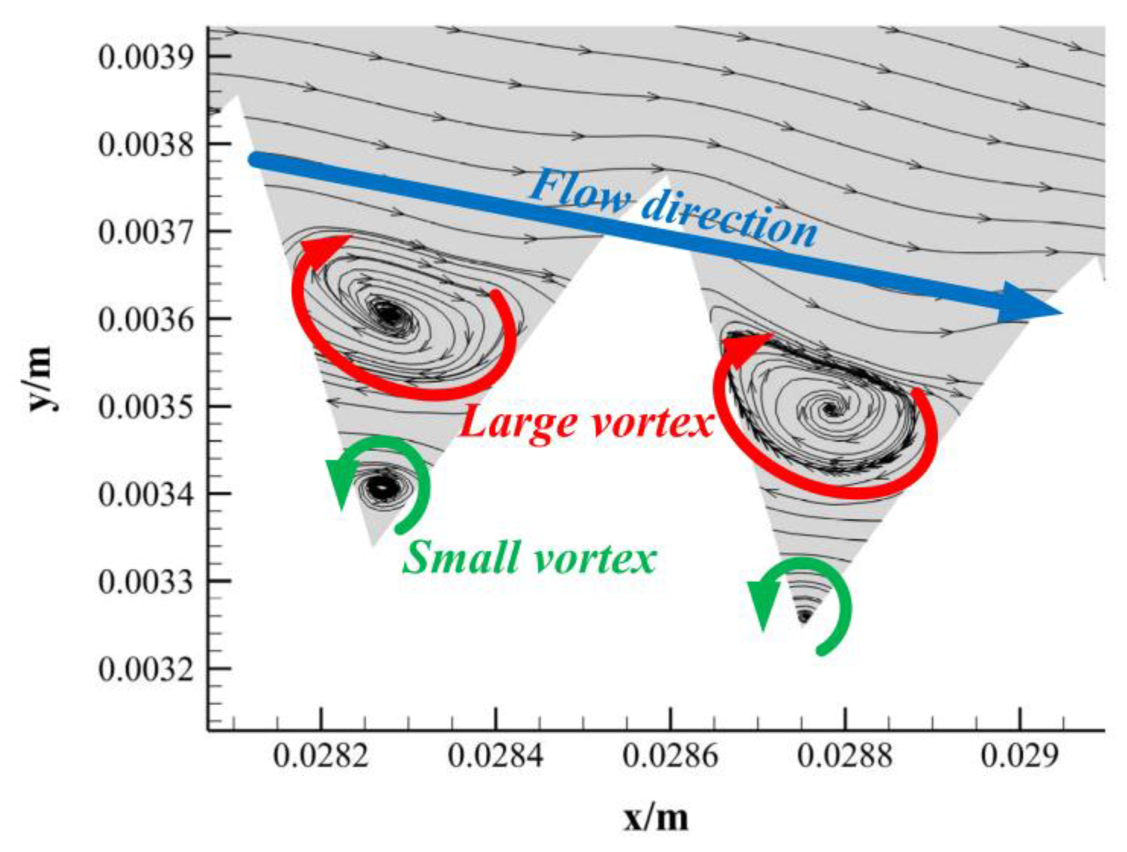
• The key to noise reduction was the generation of the secondary vortex in the microgrooves. These secondary flow vortices played a similar role to “roller bearings”, which improved the flow field around the hydrofoil and flow in the wake field.

Because noise reduction technology with spanwise microgrooved surfaces has the advantages of simple structure, easy manufacturing, and no major structural changes, it is a promising tool with the potential to be applied in marine propulsors, marine turbine blades, and other structures. However, future studies still need to be conducted on the following issues:

• The influence of the flow velocity, angle of attack of the hydrofoil, and other parameters on the noise reduction performance.
• The optimal design of the spanwise microgrooves, including its dimensional parameters and suitable positions on the hydrofoils.

References

- Lossent, J.; Lejart, M.; Folegot, T.; Clorennec, D.; Iorio, L.D.; Gervaise, C. Underwater operational noise level emitted by a tidal current turbine and its potential impact on marine fauna. Mar. Pollut. Bull. 2018, 131, 323–334. [Google Scholar] [CrossRef] [PubMed]
- Hafla, E.; Johnson, E.; Johnson, C.N.; Preston, L.; Aldridge, D.; Roberts, J.D. Modeling underwater noise propagation from marine hydrokinetic power devices through a time-domain, velocity-pressure solution. J. Acoust. Soc. Am. 2018, 143, 3242–3253. [Google Scholar] [CrossRef] [PubMed]
- Harris, B.A. Turn Down the Volume: Improved Federal Regulation of Shipping Noise Is Necessary to Protect Marine Mammals. UCLA J. Environ. Law Policy 2017, 35, 206. [Google Scholar]
- Bosschers, J. A semi-empirical prediction method for broadband hull-pressure fluctuations and underwater radiated noise by propeller tip vortex cavitation. J. Mar. Sci. Eng. 2018, 6, 49. [Google Scholar] [CrossRef]
- Viitanen, V.; Hynninen, A.; Sipilä, T.; Siikonen, T. DDES of wetted and cavitating marine propeller for CHA underwater noise assessment. J. Mar. Sci. Eng. 2018, 6, 56. [Google Scholar] [CrossRef]
- Brooks, T.F.; Pope, D.S.; Marcolini, M.A. Airfoil Self-Noise and Prediction; NASA Reference Publication 1218; NASA Langley Research Center: Hampton, VA, USA, 1989.
- Howe, M.S. Aerodynamic noise of a serrated trailing edge. J. Fluid Struct. 1991, 5, 33–45. [Google Scholar] [CrossRef]
- Howe, M.S. Noise produced by a sawtooth trailing edge. J. Acoust. Soc. Am. 1991, 90, 482–487. [Google Scholar] [CrossRef]
- Gruber, M.; Joseph, P.F.; Chong, T.P. On the mechanisms of serrated airfoil trailing edge noise reduction. In Proceedings of the 17th AIAA/CEAS Aeroacoustics Conference, Portland, OR, USA, 5–8 June 2011; p. 2781. [Google Scholar]
- Sandberg, R.D.; Jones, L.E. Direct numerical simulations of low Reynolds number flow over airfoils with trailing-edge serrations. J. Sound Vib. 2011, 330, 3818–3831. [Google Scholar] [CrossRef]
- Chong, T.P.; Joseph, P.F. An experimental study of airfoil instability tonal noise with trailing edge serrations. J. Sound Vib. 2013, 332, 6335–6358. [Google Scholar] [CrossRef]
- Jaron, R.; Moreau, A.; Guérin, S.; Schnell, R. Optimization of trailing-edge serrations to reduce open-rotor tonal interaction noise. J. Fluid Eng. 2018, 140, 021201. [Google Scholar] [CrossRef]
- Lee, H.M.; Lu, Z.; Lim, K.M.; Xie, J.; Lee, H.P. Quieter propeller with serrated trailing edge. Appl. Acoust. 2019, 146, 227–236. [Google Scholar] [CrossRef]
- Chong, T.P.; Joseph, P.F.; Gruber, M. Airfoil self noise reduction by non-flat plate type trailing edge serrations. Appl. Acoust. 2013, 74, 607–613. [Google Scholar] [CrossRef]
- Chong, T.P.; Dubois, E. Optimization of the poro-serrated trailing edges for airfoil broadband noise reduction. J. Acoust. Soc. Am. 2016, 140, 1361–1373. [Google Scholar] [CrossRef]
- León, C.A.; Ragni, D.; Pröbsting, S.; Scarano, F.; Madsen, J. Flow topology and acoustic emissions of trailing edge serrations at incidence. Exp. Fluids 2016, 57, 91. [Google Scholar] [CrossRef]
- Avallone, F.; Van der Velden, W.C.P.; Ragni, D. Benefits of curved serrations on broadband trailing-edge noise reduction. J. Sound Vib. 2017, 400, 167–177. [Google Scholar] [CrossRef]
- Avallone, F.; Van der Velden, W.C.P.; Ragni, D.; Casalino, D. Noise reduction mechanisms of sawtooth and combed-sawtooth trailing-edge serrations. J. Fluid Mech. 2018, 848, 560–591. [Google Scholar] [CrossRef]
- Clair, V.; Polacsek, C.; Garrec, T.L.; Reboul, G.; Gruber, M.; Joseph, P. Experimental and numerical investigation of turbulence-airfoil noise reduction using wavy edges. AIAA J. 2013, 51, 2695–2713. [Google Scholar] [CrossRef]
- Narayanan, S.; Chaitanya, P.; Haeri, S.; Joseph, P.; Kim, J.W.; Polacsek, C. Airfoil noise reductions through leading edge serrations. Phys. Fluids 2015, 27, 025109. [Google Scholar] [CrossRef]
- Chaitanya, P.; Joseph, P.; Narayanan, S.; Kim, J.W. Aerofoil broadband noise reductions through double-wavelength leading-edge serrations: A new control concept. J. Fluid Mech. 2018, 855, 131–151. [Google Scholar] [CrossRef]
- Chen, W.; Qiao, W.; Tong, F.; Wang, L.; Wang, X. Experimental investigation of wavy leading edges on rod-aerofoil interaction noise. J. Sound Vib. 2018, 422, 409–431. [Google Scholar] [CrossRef]
- Shi, W.; Atlar, M.; Rosli, R.; Aktas, B.; Norman, R. Cavitation observations and noise measurements of horizontal axis tidal turbines with biomimetic blade leading-edge designs. Ocean Eng. 2016, 121, 143–155. [Google Scholar] [CrossRef]
- Liu, Y.; Li, Y.; Shang, D. The Hydrodynamic Noise Suppression of a Scaled Submarine Model by Leading-Edge Serrations. J. Mar. Sci. Eng. 2019, 7, 68. [Google Scholar] [CrossRef]
- Wang, C. Trailing edge perforation for interaction tonal noise reduction of a contra-rotating fan. J. Vib. Acoust. 2018, 140, 021016. [Google Scholar] [CrossRef]
- Maizi, M.; Mohamed, M.H.; Dizene, R.; Mihoubi, M.C. Noise reduction of a horizontal wind turbine using different blade shapes. Renew. Energy 2018, 117, 242–256. [Google Scholar] [CrossRef]
- Carpio, A.R.; Martínez, R.M.; Avallone, F.; Ragni, D.; Snellen, M.; Van der Zwaag, S. Experimental characterization of the turbulent boundary layer over a porous trailing edge for noise abatement. J. Sound Vib. 2019, 443, 537–558. [Google Scholar] [CrossRef]
- Arnold, B.; Lutz, T.; Krämer, E.; Rautmann, C. Wind-Turbine Trailing-Edge Noise Reduction by Means of Boundary-Layer Suction. AIAA J. 2018, 5, 1843–1854. [Google Scholar] [CrossRef]
- Walsh, M.; Weinstein, L. Drag and heat transfer on surfaces with small longitudinal fins. In Proceedings of the 11th Fluid and Plasma Dynamics Conference, Seattle, WA, USA, 10–12 July 1978; p. 1161. [Google Scholar]
- Walsh, M. Turbulent boundary layer drag reduction using riblets. In Proceedings of the 20th Aerospace Sciences Meeting, Orlando, FL, USA, 11–14 January 1982; p. 169. [Google Scholar]
- Choi, K.S. Smart Flow Control with Riblets. Adv. Mater. Res. 2013, 745, 27–40. [Google Scholar] [CrossRef]
- Choi, K.S. Near-wall structure of a turbulent boundary layer with riblets. J. Fluid Mech. 1989, 208, 417–458. [Google Scholar] [CrossRef]
- Joslin, R.D.; Thomas, R.H.; Choudhari, M.M. Synergism of flow and noise control technologies. Prog. Aerosp. Sci. 2005, 41, 363–417. [Google Scholar] [CrossRef]
- Gillcrist, M.C.; Reidy, L.W. Drag and Noise Measurements on an Underwater Vehicle with a Riblet Surface Coating; Naval Ocean Systems Center (NOSC): San Diego, CA, USA, 1989. [Google Scholar]
- Shi, X.; Song, B.; Shi, Z. Experimental study on flow-noise reduction by riblets. J. Northwest. Polytech. Univ. 1997, 15, 395–398. (In Chinese) [Google Scholar]
- Fu, Y.F.; Yuan, C.Q.; Bai, X.Q. Marine drag reduction of shark skin inspired riblet surfaces. Biosurf. Biotribol. 2017, 3, 11–24. [Google Scholar] [CrossRef]
- Chen, D.; Liu, Y.; Chen, H.; Zhang, D. Bio-inspired drag reduction surface from sharkskin. Biosurf. Biotribol. 2018, 4, 39–45. [Google Scholar] [CrossRef]
- Luo, Y. Recent progress in exploring drag reduction mechanism of real sharkskin surface: A review. J. Mech. Med. Biol. 2015, 15, 1530002. [Google Scholar] [CrossRef]
- Luo, Y.H.; Li, X.; Zhang, D.Y.; Liu, Y.F. Drag reducing surface fabrication with deformed sharkskin morphology. Surf. Eng. 2016, 32, 157–163. [Google Scholar] [CrossRef]
- Lee, S.J.; Jang, Y.G. Control of flow around a NACA 0012 airfoil with a micro-riblet film. J. Fluid. Struct. 2005, 20, 659–672. [Google Scholar] [CrossRef]
- Chamorro, L.P.; Arndt, R.E.A.; Sotiropoulos, F. Drag reduction of large wind turbine blades through riblets: Evaluation of riblet geometry and application strategies. Renew. Energy 2013, 50, 1095–1105. [Google Scholar] [CrossRef]
- Zhang, Y.; Chen, H.; Fu, S.; Dong, W. Numerical study of an airfoil with riblets installed based on large eddy simulation. Aerosp. Sci. Technol. 2018, 78, 661–670. [Google Scholar] [CrossRef]
- Yuan, Y.; Yang, H.; Shi, Y.; Zuo, H. Study on drag reduction characteristics of airfoil for wind turbine with microgrooves on surface. J. Eng. Therm. 2018, 39, 1258–1266. (In Chinese) [Google Scholar]
- Kaakkunen, J.J.; Tiainen, J.; Jaatinen-Värri, A.; Grönman, A.; Lohtander, M. Nanosecond laser ablation of the trapezoidal structures for turbomachinery applications. Procedia Manuf. 2018, 25, 435–442. [Google Scholar] [CrossRef]
- Lam, K.; Lin, Y.F. Large eddy simulation of flow around wavy cylinders at subcritical Reynolds number. Int. J. Heat Fluid Flow 2008, 29, 1071–1088. [Google Scholar] [CrossRef]
- Ffowcs, J.E.; Hawkings, D.L. Sound generated by turbulence and surfaces in arbitrary motion. Philos. Trans. R. Soc. A Math. Phys. Sci. 1969, 264, 321–342. [Google Scholar]
- ANSYS. ANSYS FLUENT User’s Guide; ANSYS Inc.: Canonsburg, PA, USA, 2011. [Google Scholar]
- Hinze, J.O. Turbulence; McGraw-Hill Inc.: New York, NY, USA, 1975. [Google Scholar]
- ANSYS. ANSYS FLUENT Theory Guide; ANSYS Inc.: Canonsburg, PA, USA, 2011. [Google Scholar]
- UIUC Airfoil Coordinates Database. Available online: https://m-selig.ae.illinois.edu/ads/coord_database.html (accessed on 31 March 2019).
- Walsh, M.J. Drag characteristics of V-groove and transverse curvature riblets. In Proceedings of the Symposium on Viscous Flow Drag Reduction, Dallas, TX, USA, 7–8 November 1979. [Google Scholar]
- Walsh, M.J. Riblets as a viscous drag reduction technique. AIAA J. 1983, 21, 485–486. [Google Scholar] [CrossRef]
- Walsh, M.J. Effect of detailed surface geometry on riblet drag reduction performance. J. Aircr. 1990, 27, 572–573. [Google Scholar] [CrossRef]
- Gregory, N.; O’reilly, C.L. Low-Speed Aerodynamic Characteristics of NACA 0012 Aerofoil Section, Including the Effects of Upper-Surface Roughness Simulating Hoar Frost; HM Stationery Office: London, UK, 1973. [Google Scholar]
- Pan, J. The experimental approach to drag reduction of the transverse ribbons on turbulent flow. Acta Aerodyn. Sin. 1996, 14, 304–310. (In Chinese) [Google Scholar]