Understanding Ocean Acoustics by Eigenray Analysis

Abstract

Acoustics is important for all underwater systems for object detection, classification, surveillance systems, and communication. However, underwater acoustics is often difficult to understand, and even the most carefully conducted measurements may often give unexpected results. The use of theory and acoustic modelling in support of measurements is very important since theory tends to be better behaved and more consistent than experiments, and useful to acquire better knowledge about the physics principle. This paper, having a tutorial flair, concerns the use of ray modelling and in particular eigenray analysis to obtain increased knowledge and understanding of underwater acoustic propagation.

1. Introduction

Acoustics is important for all underwater systems for object detection, classification, surveillance, and communication. However, the reliability and performance of such systems depend on the environmental conditions: the water depth and bathymetry, the geoacoustic properties of the bottom, wind, and waves. These environmental properties are often unknown and change with time and location. The geoacoustic properties of the bottom are very important for low-frequency sound propagation and costly to acquire. Obtaining the required knowledge by experiments and measurements is important, but often time-consuming and costly and the results are sometimes of limited value since the environmental conditions are constantly changing.

Not all environmental parameters are equally important for a given situation. For instance, detailed acoustic information of the bottom is not required for high-frequency applications and when paths are not striking the surface and are independent of wind and waves. Therefore, sensitivity analysis is useful for a better understanding of the interaction between the environment and the system performance

The use of theory and acoustic modelling in support of measurements is very important. Theory tends to be better behaved and more consistent than experiments, and it is useful to acquire a better knowledge of the physics principle. This is an area of active research and a useful source for updated information is the Ocean Acoustics Library [1]. This paper studies the use of ray modelling and in particular eigenray analysis to obtain increased knowledge and understanding of underwater acoustic propagation.

2. Acoustic Modelling

Modelling acoustic propagation is an important issue in underwater acoustics, and there exist several mathematical/numerical models based on different approaches [2,3,4]. Some of the most used approaches are based on ray theory, modal expansion, or wavenumber integration techniques. Ray acoustics and ray tracing techniques are the most intuitive and often the simplest means for modelling sound propagation in the sea. Ray theory is derived from the wave equation when some simplifying assumptions are introduced and the method is essentially a high-frequency approximation. The method is sufficiently accurate for applications involving echo sounders, sonar, and communications systems. These applications normally use frequencies that satisfy the high-frequency conditions. However, ray theory can also be used at much lower frequencies as will be demonstrated later.

This article is about eigenrays and eigenray analysis, and there are at least two alternative models that can be used; the Bellhop model by Michael Porter [5], and the PlaneRay model developed by the first author of this paper [6]. Both models are designed to perform two-dimensional acoustic ray tracing for a given sound speed profile in ocean waveguides with variable absorbing boundaries and range-dependent bathymetry.

Bellhop is a beam ray-tracing model with several types of beams implemented including Gaussian and hat-shaped beams, with both geometric and physics-based spreading laws. The beam tracing techniques calculate the correct caustic phase shift and are free of singularity at caustics and with abrupt discontinuities at shadow zone boundaries.

PlaneRay is a ray-tracing program for modelling underwater acoustic propagation that can treat moderately range-varying scenarios and has capabilities much like Bellhop. The calculation starts with calculating the ray trajectories followed by a unique sorting and interpolation routine for efficient determination of a large number of eigenrays connecting a source with receivers positioned on a horizontal line. The complete acoustic field is determined by coherently summing the contributions of the eigenrays. The bottom reflectivity is modelled by plane-ray angle-dependent reflection coefficients because a stratified sub-bottom is perfectly represented by an angle-dependent reflection coefficient. The standard version of the program assumes that the bottom has a sediment layer over a half space with solid rock. Models for more complicated bottoms can be downloaded from other sources. PlaneRay is programmed in MATLAB, which gives the user an easy opportunity to study and understand the code.

3. The PlaneRay Model

PlaneRay calculates the ray trajectories, which are computed in the standard way by dividing the water column into many thin layers with a sound speed and a sound speed gradient, derived from oceanic databases or CTD measurements. This gives ray trajectories composed of circular segments. The unique feature of PlaneRay is a sorting and interpolation routine for efficient determination of a large number of eigenrays connecting a source with receivers positioned on a horizontal line. The ray theory is a high-frequency approximation, but can also be used for low frequencies, which can be demonstrated by comparison with the wavenumber integration models and models based the parabolic approximation. PlaneRay has been tested and compared with the wavenumber integration model OASES and the parametric model RAMS for an elastic bottom at showing good agreement for frequencies down to 25 Hz [7,8,9,10].

The algorithm consists of three stages

(1)

The initial ray tracing using a large number of rays to accumulate ray history out the entire sound field of interest.

(2)

Sorting the rays in classes having similar history followed by interpolating the classes independently

(3)

Synthesis of the acoustic field in the frequency domain by coherently adding the contributions of the eigenrays

This gives the acoustic field in the frequency domain, and the time responses are obtained by Fourier transformation of the frequency functions.

3.1. Ray tracing and Ray History

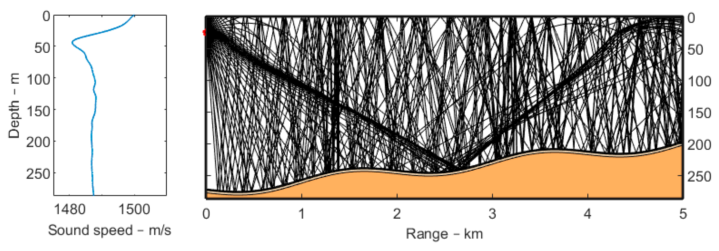
The water column is divided into a number of layers, and the computation is organised in the depth or z-direction. The algorithm makes repeated use of these equations, tracking a ray upward or downward until it reflects from an interface or turns within a layer. The program computes the trajectories of a large number of rays with the starting angles at the source covering the total water volume in the range and depth of interest to the analysis. In addition to the ray trajectories, the program finds the locations of all the surface and bottom reflections and turning points. For the geometrical transmission loss calculation, the incoming and outcoming angles of the reflection are also determined. All information is stored in the computer memory in tables of ray history.

Figure 1 shows the acoustic propagation from a source at 25 m depth over a gently undulating up-sloping bottom with an average slope angle of 2.3 degrees and a sound speed profile typical of northern waters.

For clarity, only a few rays are used in the figure, but in practice, many more are used. Crucial to the modelling accuracy is the choice of the initial angles and the density of the depth samples of the sound speed profile. Typically, the depth spacing should be less than one meter.

The ray history is stored in a script HIST with the fields:

• THETA, initial ray angle at the source
• ANGLE, ray angle at reception
• RANGE, horizontal distance
• TIME, travel time
• DISTANCE, path length
• CLASS, ray type
• COUNT, counter

3.2. Sorting and Interpolation

Generally, the initial ray tracing is not sufficient to produce the acoustic field with sufficient accuracy. The approach used in PlaneRay is based on the interpolation of the results of the initial ray tracing, and the interpolation has to be done on rays having the same type of ray history. The first task is, therefore, to sort the rays into different classes having a similar history. The classes are defined by the number of interactions with the surface and bottom and the number of turning points. The sorted classes will have relatively continuous range-angle relations and therefore be amenable to interpolation. The next step is to determine the eigenrays and their trajectories.

Table 1. Definition of classes.

Class	Bottom	Surface	Initial direction
Class 1	0	0	Direct ray
Class 2	n−1	n	Negative start angle
Class 3	n	n	Negative start angle
Class 4	n	n	Positive start angle
Class 5	n	n−1	Positive start angle
Class	Bottom reflection		Upper tuning points
Class 6	n	n+1	Negative start angle
Class 7	n	n	Negative start angle
Class 8	n	n	Positive start angle
Class 9	n+1	n	Positive start angle
Class	Surface reflection		Lower turning points
Class 10	n+1	n	Negative start angle
Class 11	n	n	Negative start angle
Class 12	n	n	Positive start angle
Class 13	n	n+1	Positive start angle
Class	Upper turning points		Lower turning points
Class 14	n	n−1	Negative start angle
Class 15	n	n	Negative start angle
Class 16	n	n	Positive start angle
Class 17	n−1	n	Positive start angle

shows the definition of classes. Class no. 1 is the direct wave going to the receiver without any contact with the surface or bottom and without going through turning points. The other 16 classes are reflected from the surface or the bottom or go through turning points n or n−1 times. In addition, we have to distinguish between starting with rays that start with a positive angle (downwards) or negative angles (upwards). In total there are, in addition to the direct wave, 16 different combinations of classes of ray history. With a flat bottom, this is the maximum number of possible cases, but there may be more cases when the depth changes significantly with the range, but the program will look for and add such cases.

3.3. Intensity and Transmission Loss Calculations

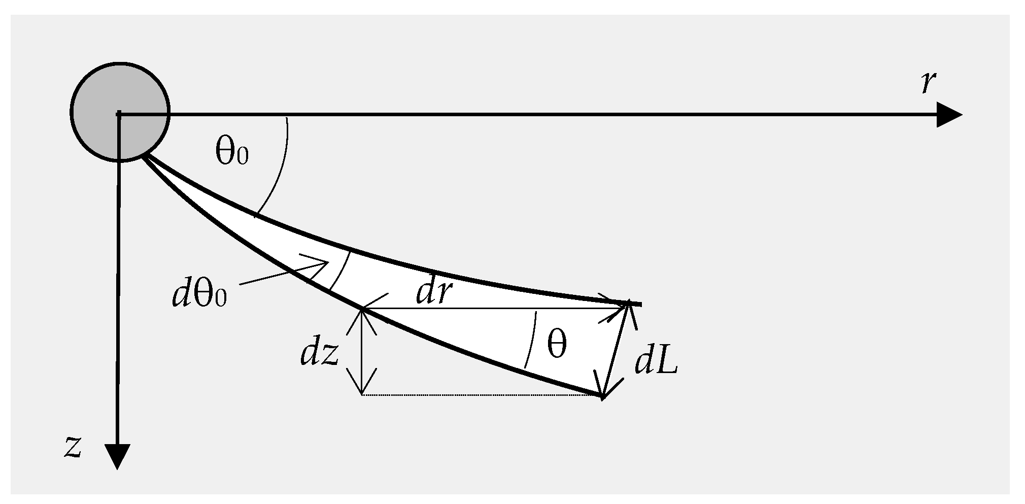
The sorted and interpolated results are computed for each of the classes and used to calculate the sound intensity based on the principle that energy radiated in a narrow tube remains inside the tube as indicated in Figure 2. Here r₀ represents a reference distance and θ₀ is the initial ray angle at the source, dθ₀ is the initial angular separation between two rays, dr is the incremental range increase, θ is the angle at the field point, dz is the depth differential, and dL is the width of the ray tube. The intensity is then expressed as:

$$\frac{I}{I_0}=\frac{r_0^2}{r}\frac{\cos {\theta }_0}{\cos \theta }\left|\frac{d{\theta }_0}{dz}\right|=\frac{r_0^2}{r}\frac{c}{c_0}\left|\frac{d{\theta }_0}{dz}\right|,$$

(1)

where I₀ is the intensity at the reference distance r₀. With reference to the distance r₀, the transmission loss TL is expressed as:

$$TL=10{\log }_{10}\left(\frac{r}{r_0^2}\right)+10{\log }_{10}\left|\frac{dz}{d{\theta }_0}\right|+10{\log }_{10}\left(\frac{c}{c_0}\right),$$

(2)

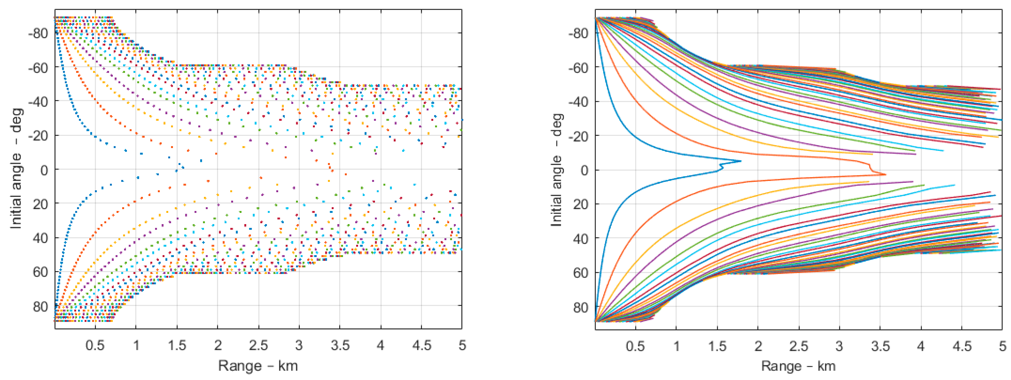
The main problem with using ray history for calculating eigenrays is the calculation of the incremental range increase for a given change in the initial ray angle. A plot of the trajectory of a single initial angle is a, in general, discontinuous function not suited for interpolation. The sorted classes will have relatively continuous range-angle relations and therefore be amenable to interpolation. The calculation of the derivative $dz/d\theta$ is performed using the sorted and interpolated values to ensure high accuracy of the estimates.

A plot of range versus the initial angle is shown in Figure 3. Each dot represents the intersection with a depth layer as a function of the ray angle at the source. The dots give the impression to be partly organised and not completely random (left panel). The right panel of Figure 3 shows an example of sorted range-angle relations.

Note that in this treatment, the transmission loss includes the geometric spreading loss, and the absorption loss must be included separately. The geometric transmission loss consists of two parts. The first term represents the horizontal spreading of the ray tube and results in a cylindrical spreading loss. The second and third terms represent the vertical spreading of the ray tube caused by the depth gradient of the sound speed. The third term can usually be ignored since the sound speed variations are small in the context of intensity calculation.

3.4. Bottom and Surface Interactions

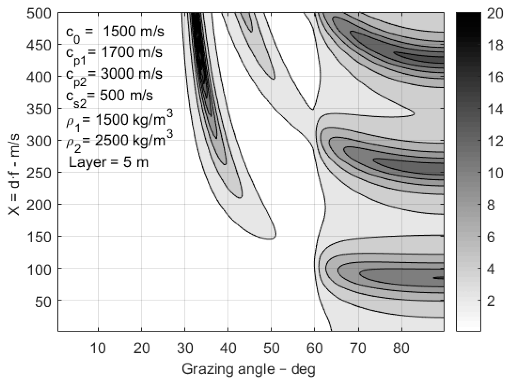
The surface reflection coefficient of the flat surface is equal to minus one, but a surface roughness caused by the ocean waves may lead to diffuse scattering and an incoherent reflection loss. The bottom reflectivity of a layered medium is generally a function of the frequency and angle. Figure 4 shows a contour display of the reflection loss for the bottom with a fluid sediment layer of thickness 5 m over an elastic half-space. The sound speed and density of the sediment layer is 1700 m/s and is 1500 kg/m³, respectively. The elastic half-space is a hard bedrock with a compressional speed of 3000 m/s, a shear speed 500 m/s, and density of 1800 kg/m³. All wave attenuations are set to 0.5 dB per wavelength. For very low frequency, the critical angle is predominately caused by the compressional speed of 3000 m/s, and for the higher frequency, the sediment sound speed of 1700 m/s is dominating.

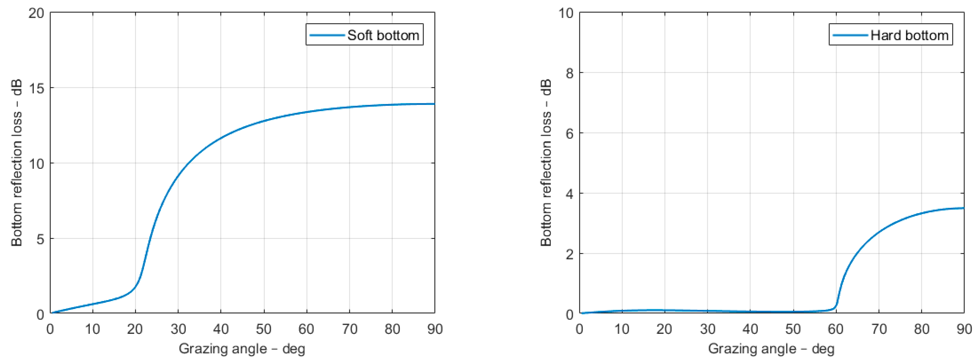
The examples considered in this paper are based on two types of bottoms: a soft bottom and a hard bottom with the parameters given in

Table 2. Parameters for soft and hard bottoms.

Bottom Type	Compressional Speed (m/s)	Shear Speed (m/s)	Density (kg/m3)
Soft	1700	0	1500
Hard	3000	200	2500

. The sound speed of the water is 1500 m/s, and the density is 1000 kg/m³. The bottom attenuations for both compressional and shear waves are set to 0.5 dB per wavelength.

The reflections from the bottom are treated with a hybrid approach whereby the bottom interaction is modelled using plane wave reflection coefficients since any arbitrary stratified sub-bottom is perfectly represented by an angle-dependent reflection coefficient. Figure 5 shows an example of the bottom reflection loss in dB as a function of the grazing angle for the two bottom cases, soft and hard as defined in Table 2. The critical angle, which for a bottom with sound speed c_b and water speed c_w, is defined by:

$${\theta }_{crit}={\cos }^{-1}\left(c_w/c_b\right),$$

(3)

where c_w < c_b, which is nearly always true underwater and almost never true in air acoustics, the critical angle is real and most important for the understanding of the underwater acoustics.

4. Eigenrays

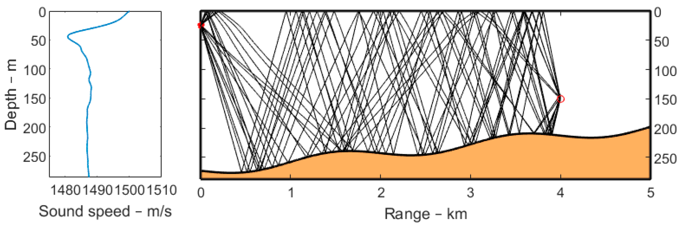
The program first computes the trajectories of a large number of rays with the starting angles at the source covering the total water volume in the range and depth of interest to the analysis. The program computes the locations and striking angles of all the surface and bottom reflections and the geometrical transmission loss. All information is stored in the computer memory in tables of ray history, and all the eigenrays. Figure 6 shows an example of the eigenrays from a source at 25 m depth to a target or receiving point at 150 m depth at a range of 4 km.

The eigenray contributions are denoted by $p_n\left(r,z,\omega \right)$ and the total sound pressure is expressed as a coherent sum of eigenrays:

$$p(r,z,\omega )={\displaystyle {\sum }_{n=1}^N{p}_n^{}}\left(r,z,\omega \right).$$

(4)

The eigenrays are dependent on the sound speed profile and the bathymetry, but not on the frequency. Generally, there are several eigenrays for each combination of start and end positions as shown in Figure 6. How important these are depend on the acoustic properties of the bottom and the critical angle, as shown in the following sections.

From the stored history, the PlaneRay program computes the:

• Amplitude (1)
• Time delay (2)
• Initial angle (3)
• Receiver angle (4)

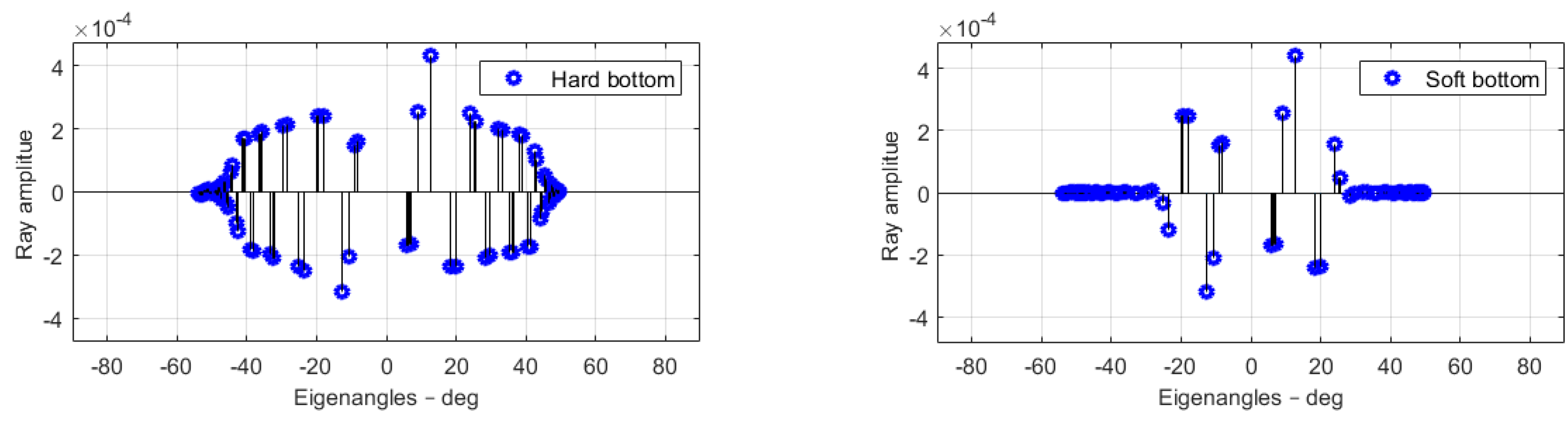
By cross-plotting various items of these elements, many interesting features of the sound field are obtained. Figure 7 shows a cross plot of amplitudes (1) and initial angle (3), the amplitudes of the eigenrays as a function of initial eigenangles. The examples in Figure 7 are for a hard and soft bottom, respectively. The hard bottom has a sound speed of 3000 m/s, and a critical angle of 60°, the sound speed of the soft bottom was 1700 m/s and a critical angle of 28°. In both cases, the effect of the critical angle was evident; only eigenrays with angles lower than the critical angle were important.

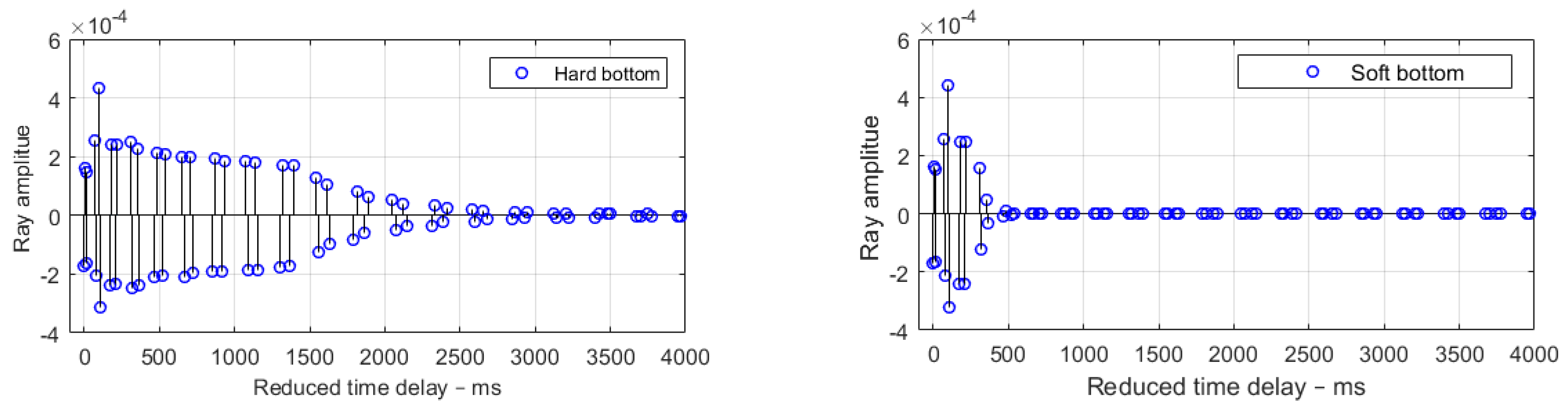
Figure 8 is a cross plot of the amplitude (1) and the time delay (2), which can be interpreted as the channel impulse response. For a hard bottom, the response is an impulse with a duration of 2000 ms. For a soft bottom, the response duration is considerably shorter of about 300 ms.

4.1. Detecting Caustics

A problem with ray theory is caustics and crossing of rays, where the basic ray theory breaks down and predicts infinite intensity. Real caustics are caused by characteristics of the sound speed profiles, or in some cases with the bathymetry. There are also so-called “false” caustics which are really artefacts often caused by too sparsely and wrongly interpolated sound speed profiles.

Some theories exist that amend and repair the defects of ray theory [11], but such theories are frequency dependent and not very useful. However, the PlaneRay model has a component that detects the locations of the turning points and caustics and avoids unnecessary mistakes in interpretation. The caustics occur when the derivative of range r with the initial angle, i.e., $dr/d\theta =0.$

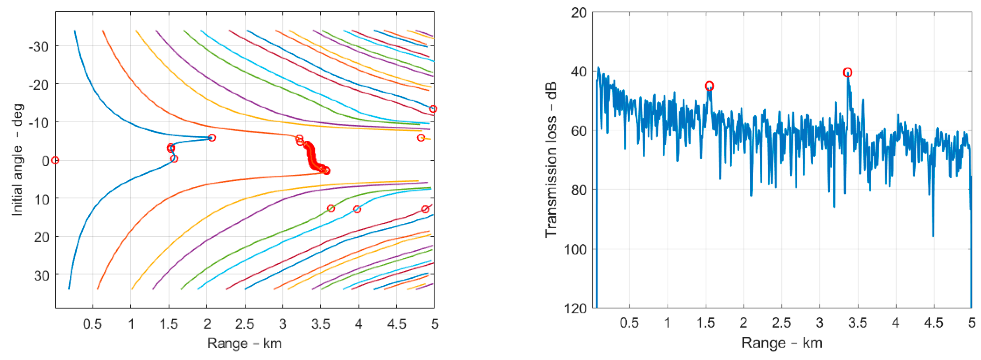
The left panel of Figure 9 illustrates a plot of the range and the initial angle with the detected caustics marked with red circles showing that the caustics are detected at ranges around 1.5 km and 3.4 km. This is demonstrated by the right panel of Figure 9 showing a transmission loss in dB as a function of range for a frequency of 100 Hz. This loss includes absorption and bottom reflection losses and predicts correctly the positions of the anomalously high sound levels at expected ranges with the caustics. Thus, the caustics are detected, which is useful, although the levels are not necessarily correct.

4.2. Modelling Particle Movements

Measurements and models of ocean acoustic wave fields are mostly concerned with sound pressure and not with particle motion, which is a vector quantity. However, there is a growing interest in particle motion driven by new developments and applications of sensor technologies. For instance, marine biologists have found that many species are more sensitive to particle motions, in addition to sound pressure [12].

Equation (4) gives the sound pressure as a coherent sum of eigenray contributions or multipath contributions. The eigenrays are plane waves with the property that the particle velocity is the sound pressure divided by the specific acoustic impedance. The particle velocity is proportional to the gradient of the sound pressure, and therefore the horizontal and vertical components of the particle velocities are found by:

$$\begin{array}{l}v(r,z,\omega )=\frac{1}{\rho c}\cdot {\displaystyle {\sum }_{n=1}^N{p}_n}\left(r,z,\omega \right)\cos \left({\beta }_n\right)\\ u(r,z,\omega )=\frac{1}{\rho c}\cdot {\displaystyle {\sum }_{n=1}^N{p}_n}\left(r,z,\omega \right)\sin \left({\beta }_n\right)\end{array}$$

(5)

where β_n are the ray angles with the horizontal at the receiver shown in Figure 7 for the two bottom types treated here. In addition, it is useful to introduce the nominal particle velocity as:

$${\nu }_{nom}(r,z,\omega )=\frac{1}{\rho c}\cdot {\displaystyle {\sum }_{n=1}^N{p}_n}\left(r,z,\omega \right).$$

(6)

This velocity is nominal in the sense that the particle velocity is obtained by directly converting pressure to velocity by dividing with the acoustic impedance.

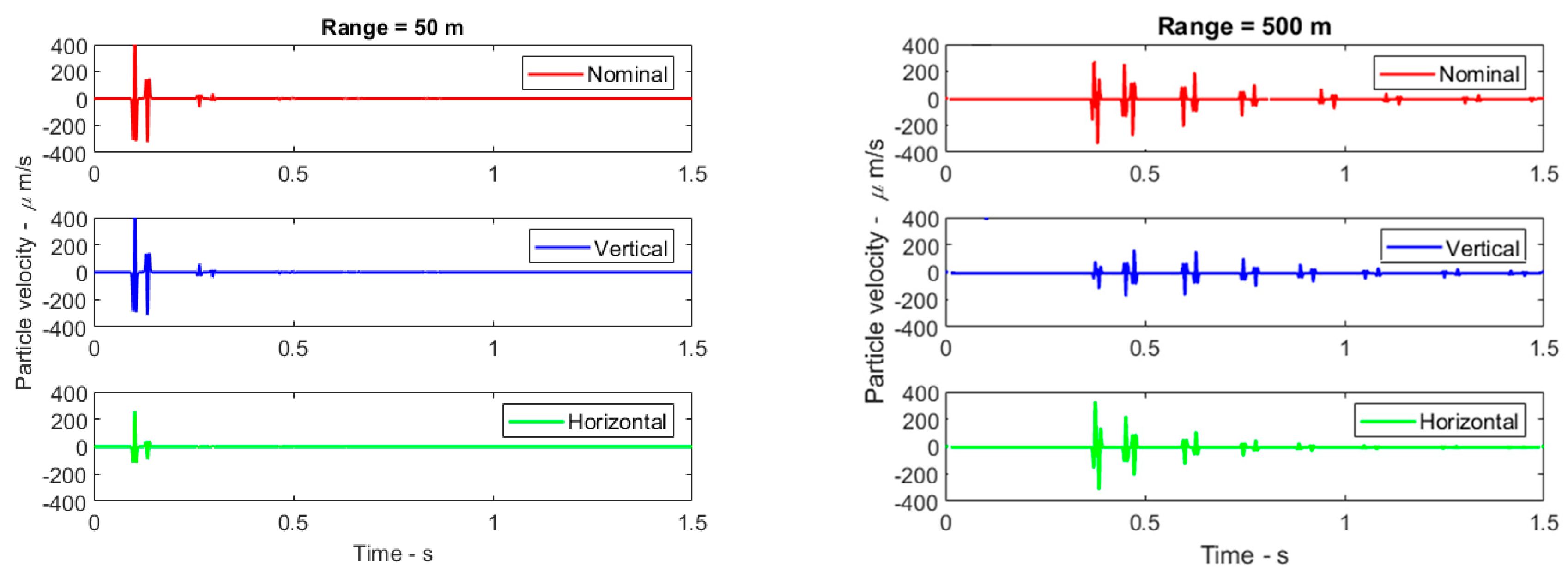
Figure 10 shows the impulse amplitudes (µm/s) at ranges of 50 m and 500 m for the nominal, vertical, and horizontal particle velocities. The impulses are calculated for a source pulse with a peak pressure of 200 dB at 1 µPa. The horizontal response is stronger than the vertical response for distances longer than the water depth when ray angles are closer to the horizontal plane. Notice also that the nominal responses are stronger, but of the same order of magnitude as the amplitudes of the vertical and horizontal responses.

4.3. Using the Reciprocity Principle for Moving Sources

In many cases, a survey is conducted with a moving source transmitting signals to a stationary receiver. This is opposite to that of most propagation models, including PlaneRay, which assumes a stationary source and a moving receiver. In the case of a flat bottom, it is not a problem since the reciprocity principle states that the source and receiver can switch positions giving the same result. However, this is not true in range-dependent situations.

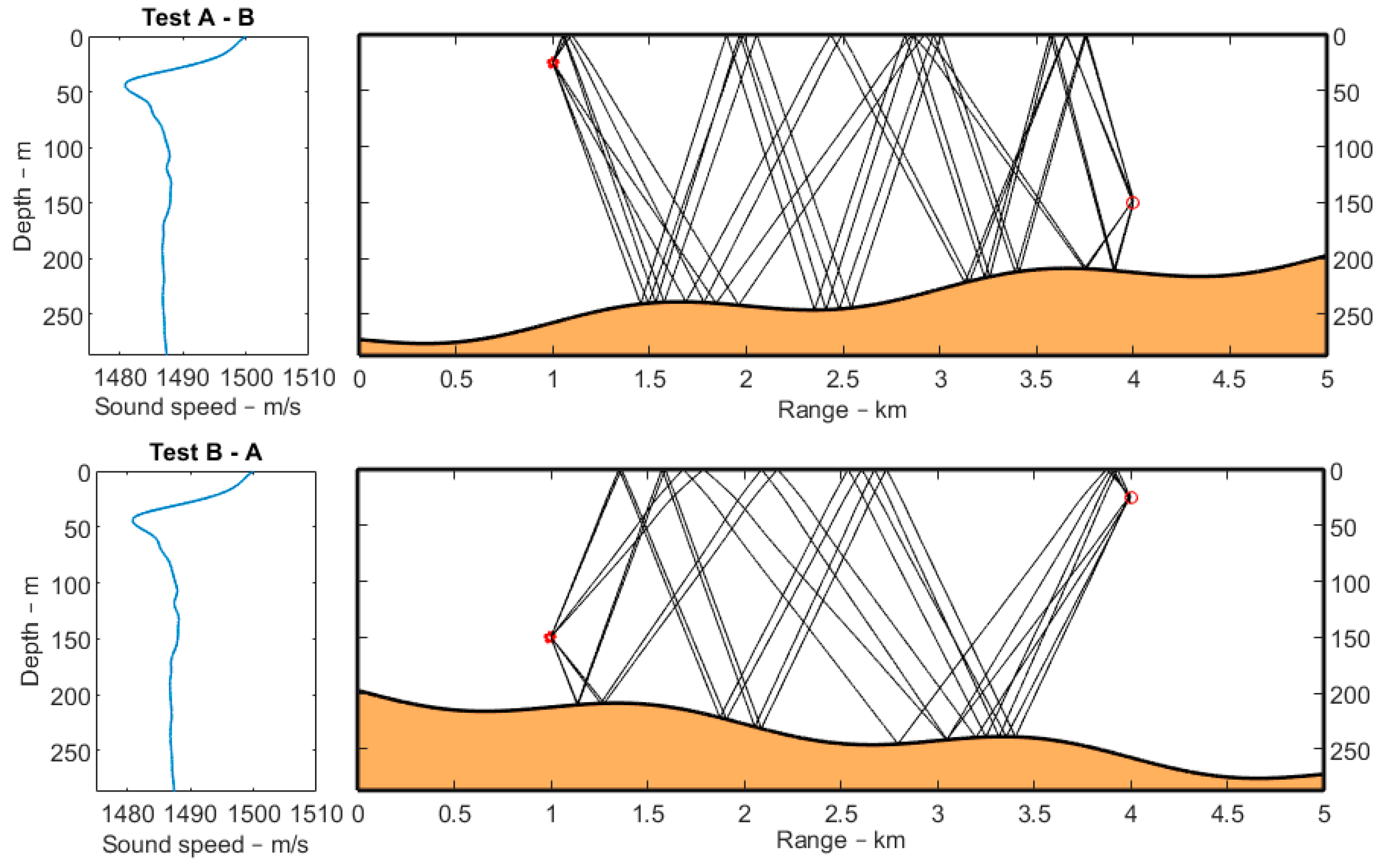
Consider the example where a moving source at position A at a depth of 25 m is transmitting to a stationary receiver in position B at a depth of 150 m. Since the bottom is gently sloping upwards, the results of computing the transmission loss directly from A to B in one single step is not valid. Instead, one will obtain a valid result of using several computations with the source in different ranges along the track, which can be time-consuming. However, valid results are obtained with a single computation by interchanging the source and the receiver and by left-right flipping of the bathymetry, as illustrated in Figure 11. The ray paths in the two plots are identical and therefore produce the same acoustic fields.

4.4. Bathymetric Effects and Long Range Propagation: An Example from Seismic

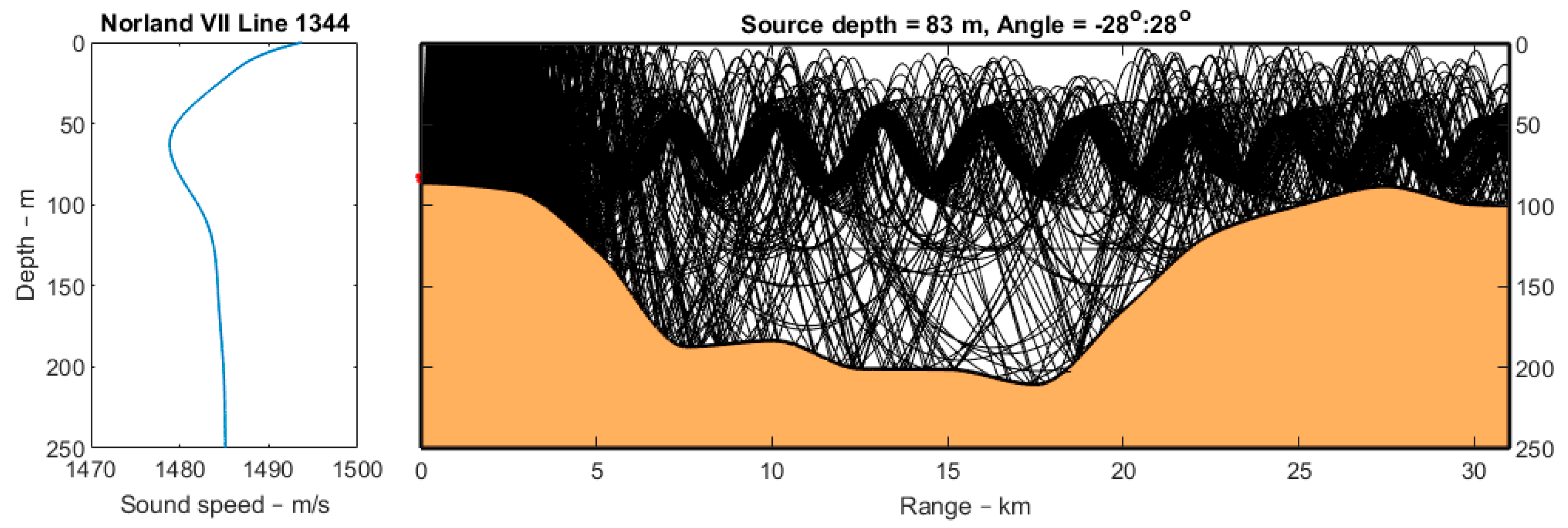
A recent seismic survey in Vesteraalen, Norway used an airgun array at approximately 6 m depth as the source and a towed hydrophone array as the receiver and recorded the sound over a distance of 35 km. In addition, a stationary receiving hydrophone was deployed at a depth of 83 m which was directly below the towing line. The data received on this hydrophone were analysed, compared, and discussed here with the modelled data (see also [13] for more details). Since the source is moving, in this case, the reciprocal scenario technique is applied by flipping the bathymetry and interchanging the depths of the source and the receiver, as described earlier. The modelled scenario is shown in Figure 12 with the sound speed profile, the bathymetry, and some of the ray trajectories.

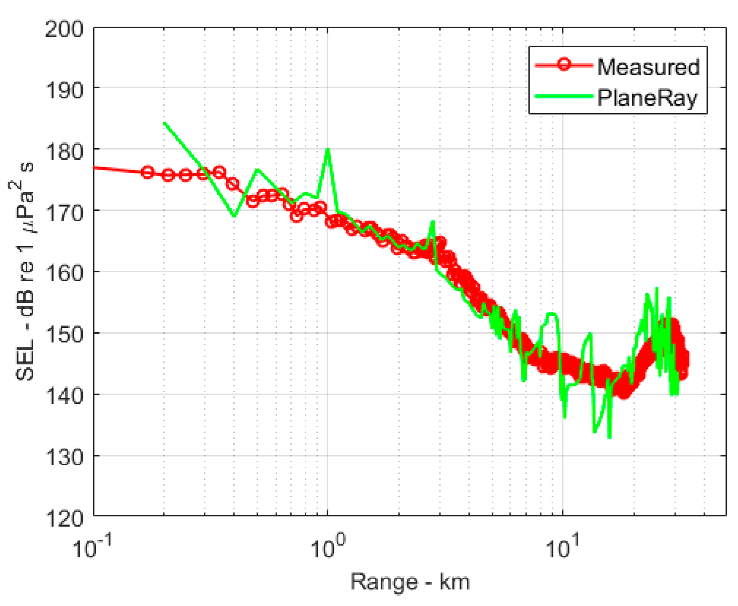
The water depth varies significantly over the track, which makes the modelling very difficult. This is evident from Figure 13, which shows the measured and modelled SEL (Sound Exposure Level) [14] as a function of the range. The effect of the bathymetry is evident. With increasing water depth, the sound decays rapidly with the range, but at the end of the track approaching 30 km, the sound level increases again. The agreement between the measured and modelled values is not very good in such a complicated case mainly because of the numerical difficulties in calculating the eigenrays.

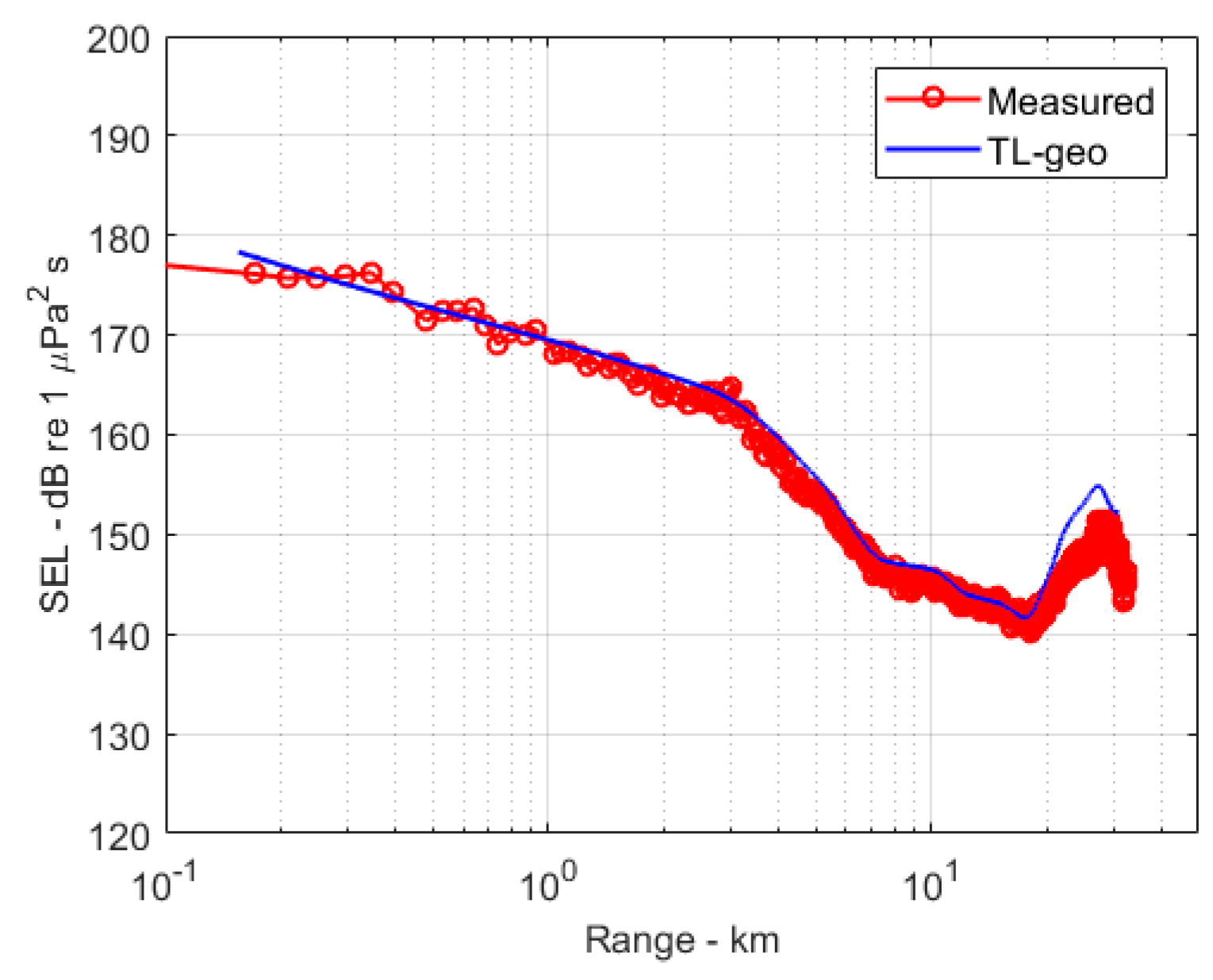
Interestingly, better agreement with the measured values is obtained by using a simple geometrical expression given by:

$$T{L}_{geo}=10{\log }_{10}\left(\frac{r^2}{\sqrt{1+{\left(\frac{r}{r_0}\right)}^2}}\right)+10{\log }_{10}{\left(\frac{D\left(r\right)}{D\left(r=1\right)}\right)}^4.$$

(7)

There is no proof for this expression, but it postulates that the transmission loss is purely geometric and is composed of two parts. Close to the source where r < r₀, the transmission loss is dominated by spherical spreading going gradually over to cylindrical spreading as r > r₀. The parameter r₀ specifies the transitional range between spherical to cylindrical, in this case, is set equal to the water depth at the source. The second part of the equation accounts for bathymetry or depth, D(r), representing the “thinning” of the ray density with increasing depth. Equation (7) is an expression that includes both near and far field effects and the effects of the bathymetry and is in good agreement with the measurements as shown in Figure 14. The agreement indicates that the sound level at long ranges, and after many bottom and surface reflections, is mostly dependent on the bathymetry.

5. Summary and Conclusion

This paper has demonstrated examples of how eigenray analysis could be used to obtain a better understanding of the underwater acoustic propagation problems. The examples are produced using the ray-tracing model PlaneRay, which has a unique algorithm of sorting and interpolation for the efficient determination of a large number of eigenrays connecting a source with receivers positioned on a horizontal line. The acoustics field is found by the coherent summation of all eigenray contributions. The use of eigenray analysis is demonstrated by examples from typical oceanic environments with up-sloping and slightly undulating different bottom parameters. The examples include the importance of the critical angles for transmission over long ranges and only rays striking the bottom with angles lower than the bottom critical angles give a significant contribution to the acoustic field.

Acoustic modelling programs normally assume a stationary source and a moving receiver. This is the opposite of what is used in geophysical surveys, which are conducted with a towed source and a fixed receiver. The paper has demonstrated how the reciprocity principle can be used for efficient modelling of such cases. The program has an algorithm for detection of caustics, which is important for quality control and determination of range intervals where the ray theory breaks down. An example propagation 30 km long rack with significant depth variation is modelled and compared with measurements and with a new formula for the transmission loss calculation, which includes the effects of the bathymetry, in addition to the near and far field effects.