On Tidal Current Velocity Vector Time Series Prediction: A Comparative Study for a French High Tidal Energy Potential Site


Abstract
:1. Introduction
2. Description of the Computational Methods
2.1. Numerical Model
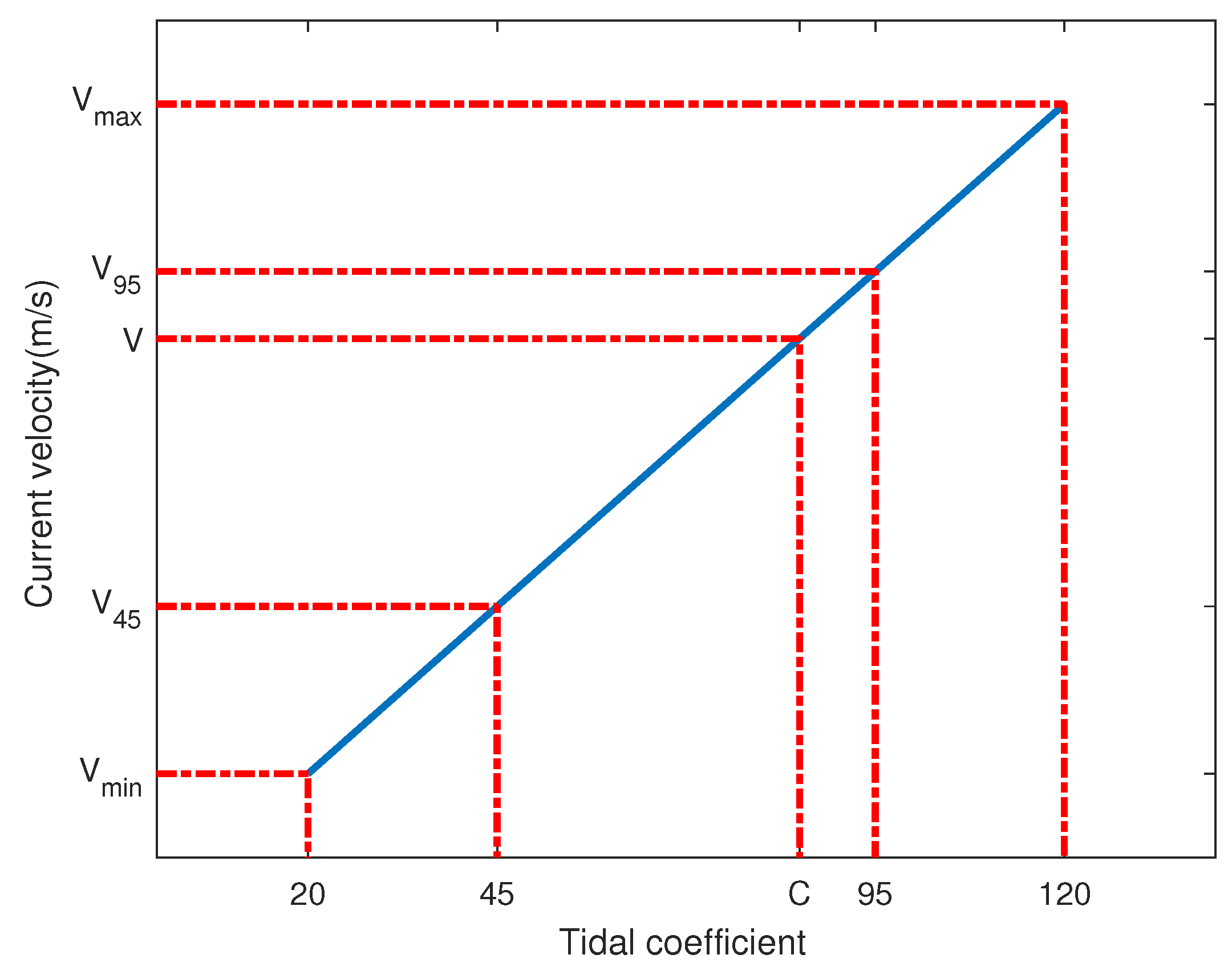
2.2. Linear Approximation
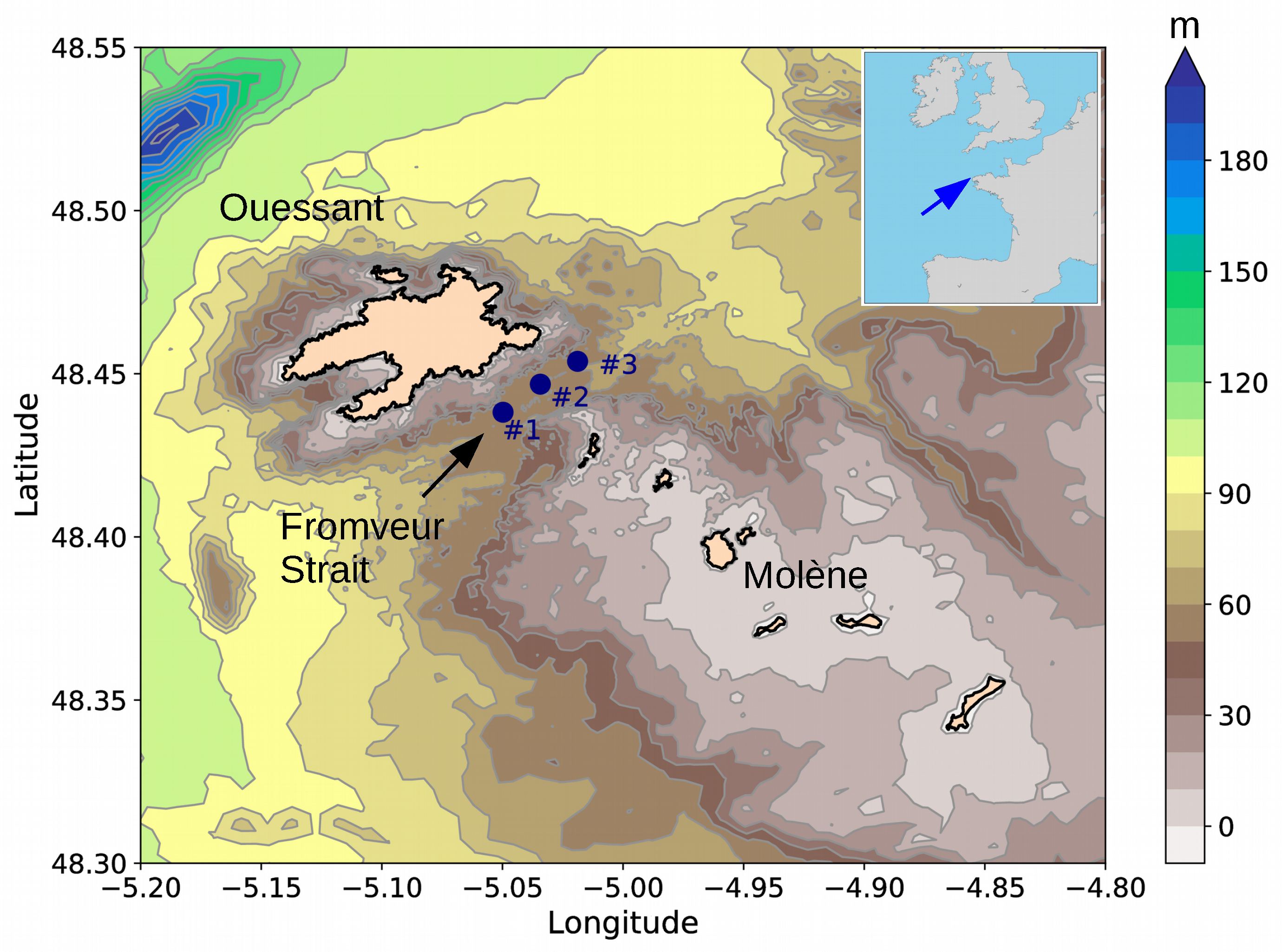
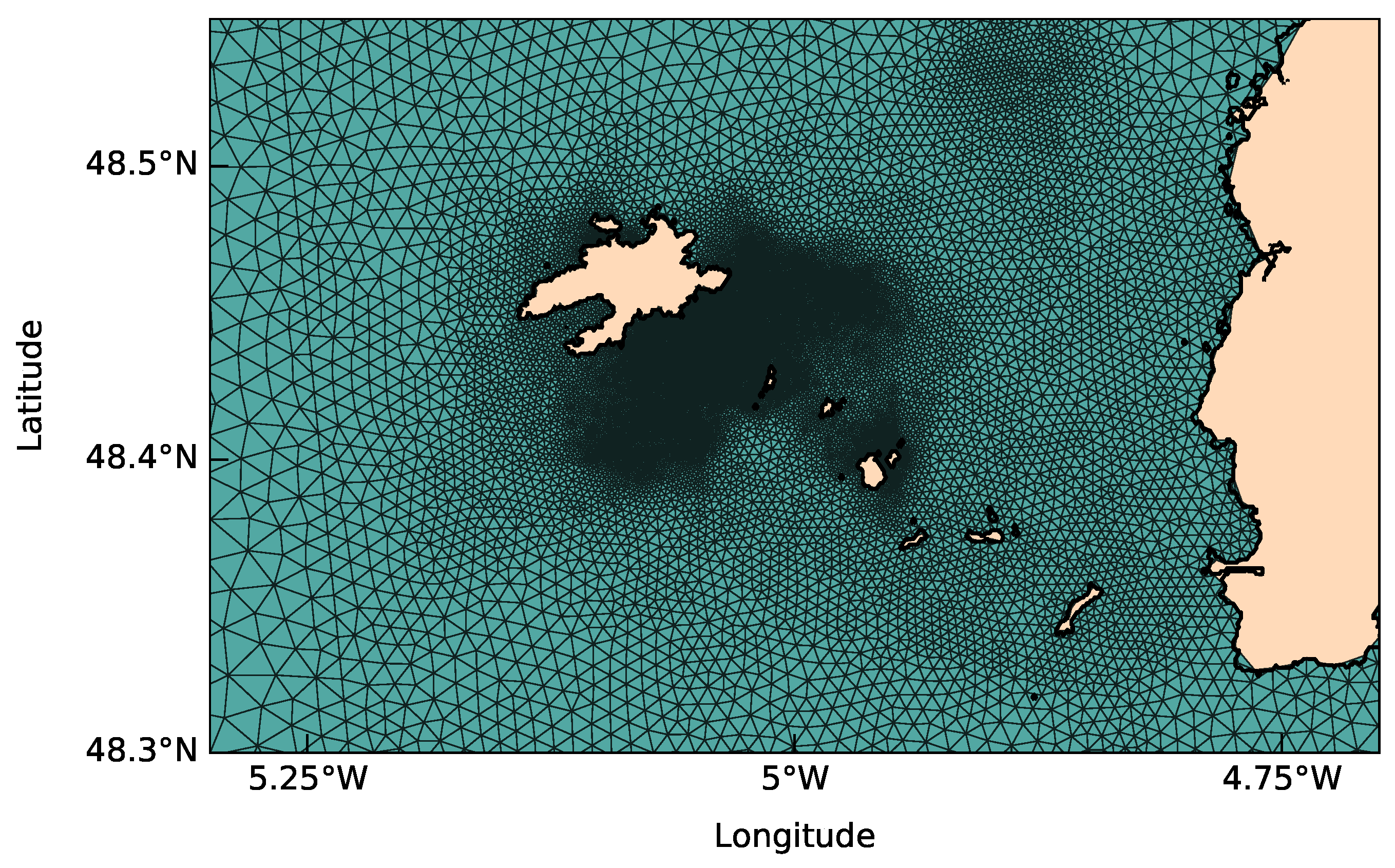
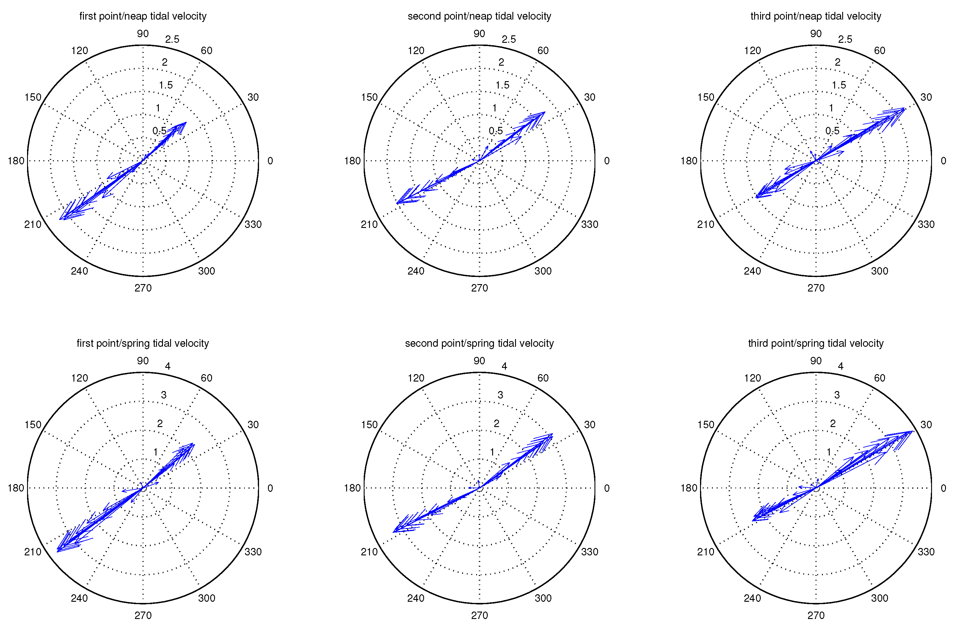
3. Site Description and Selected Locations
4. Discussions about the Results
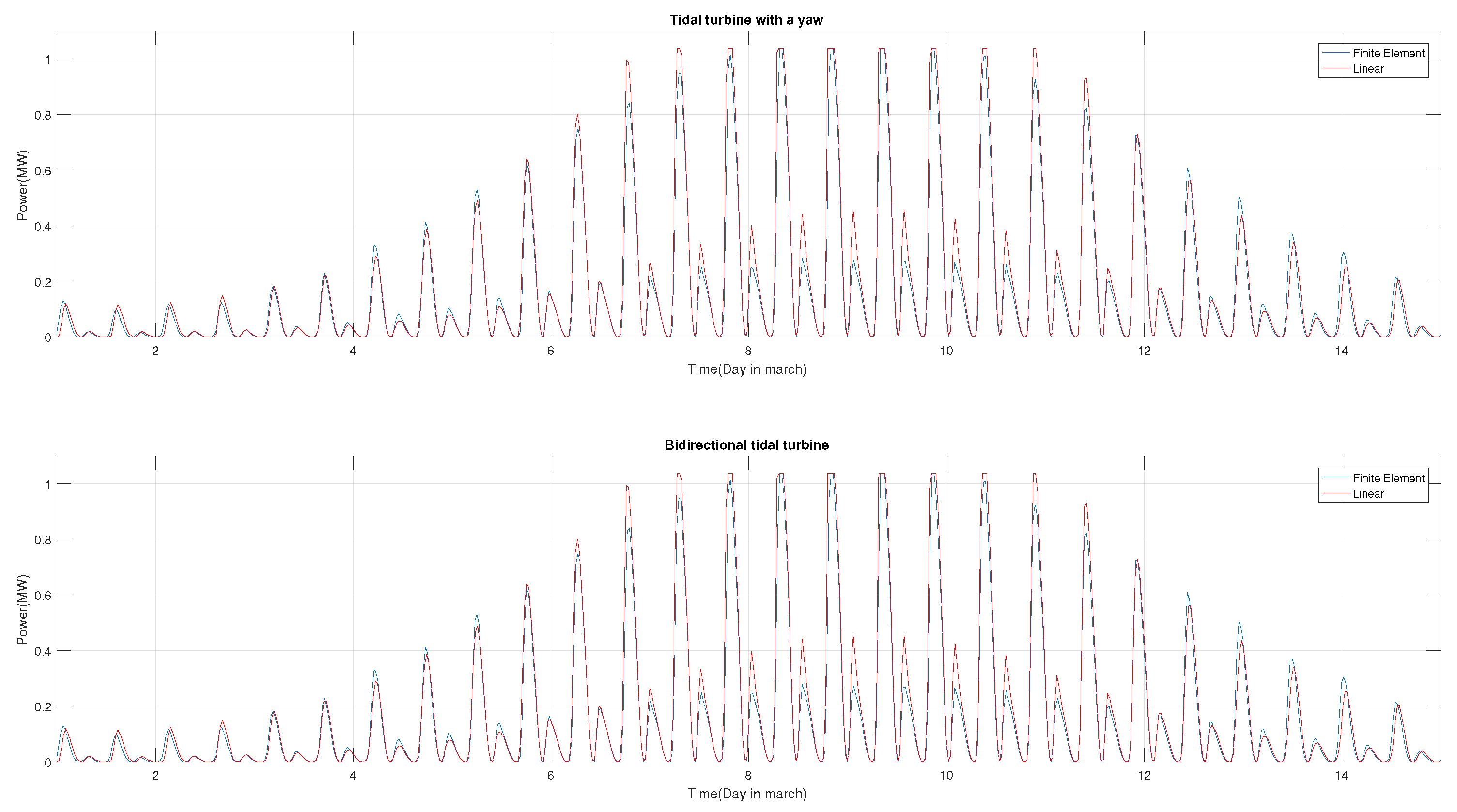
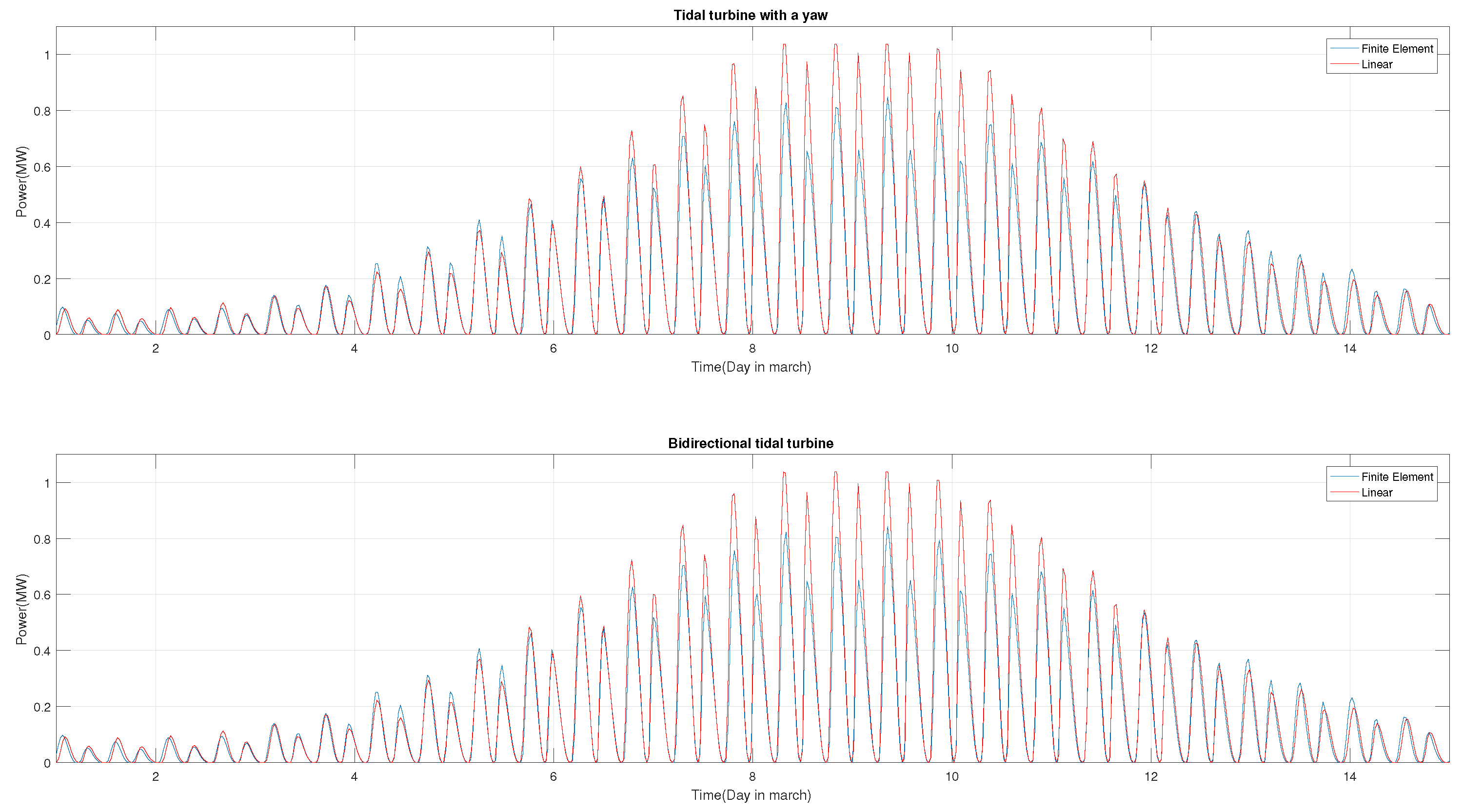
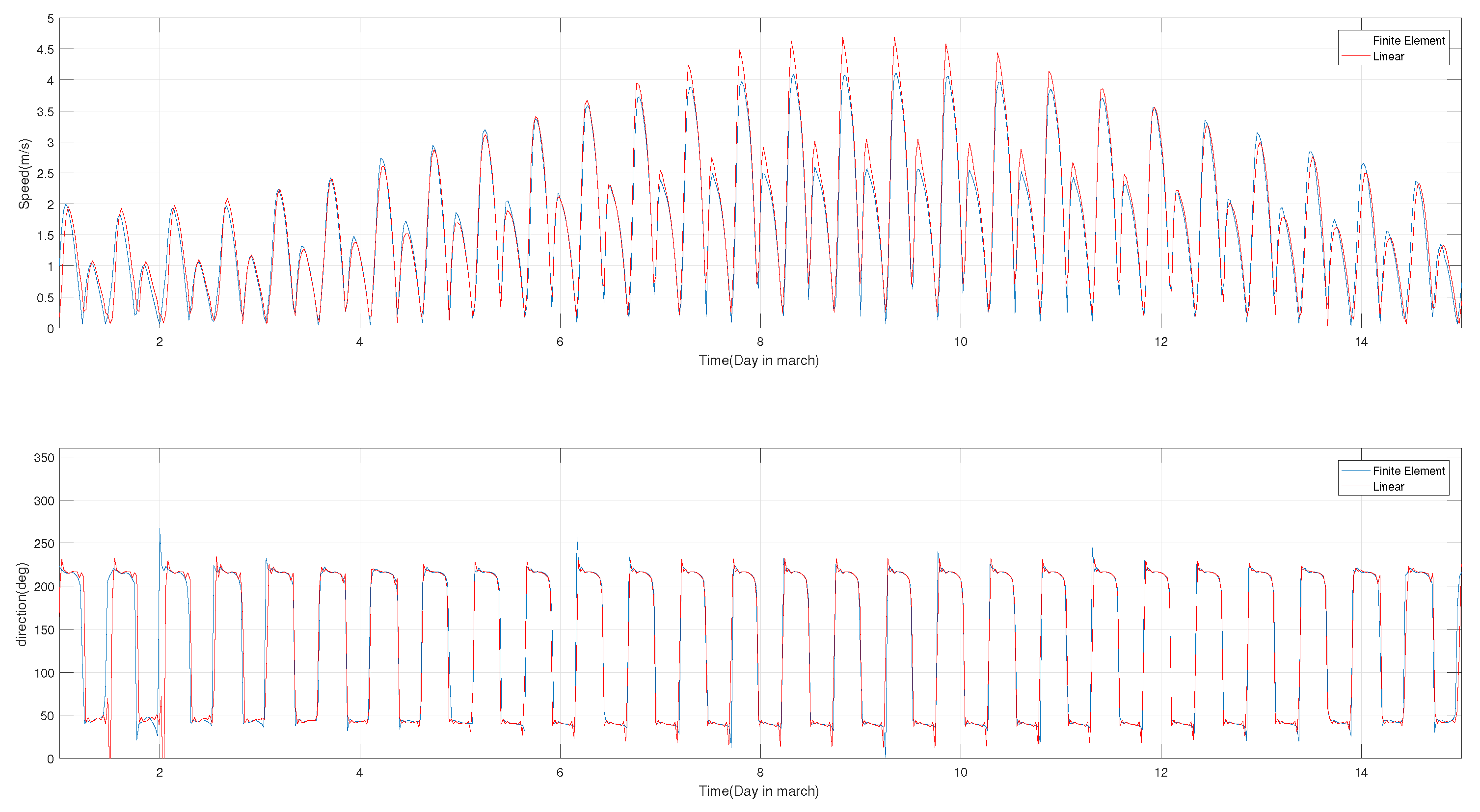
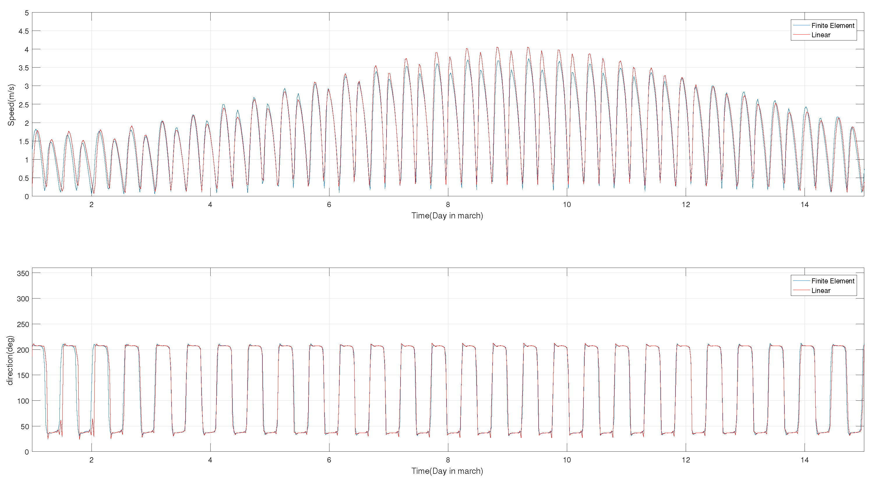
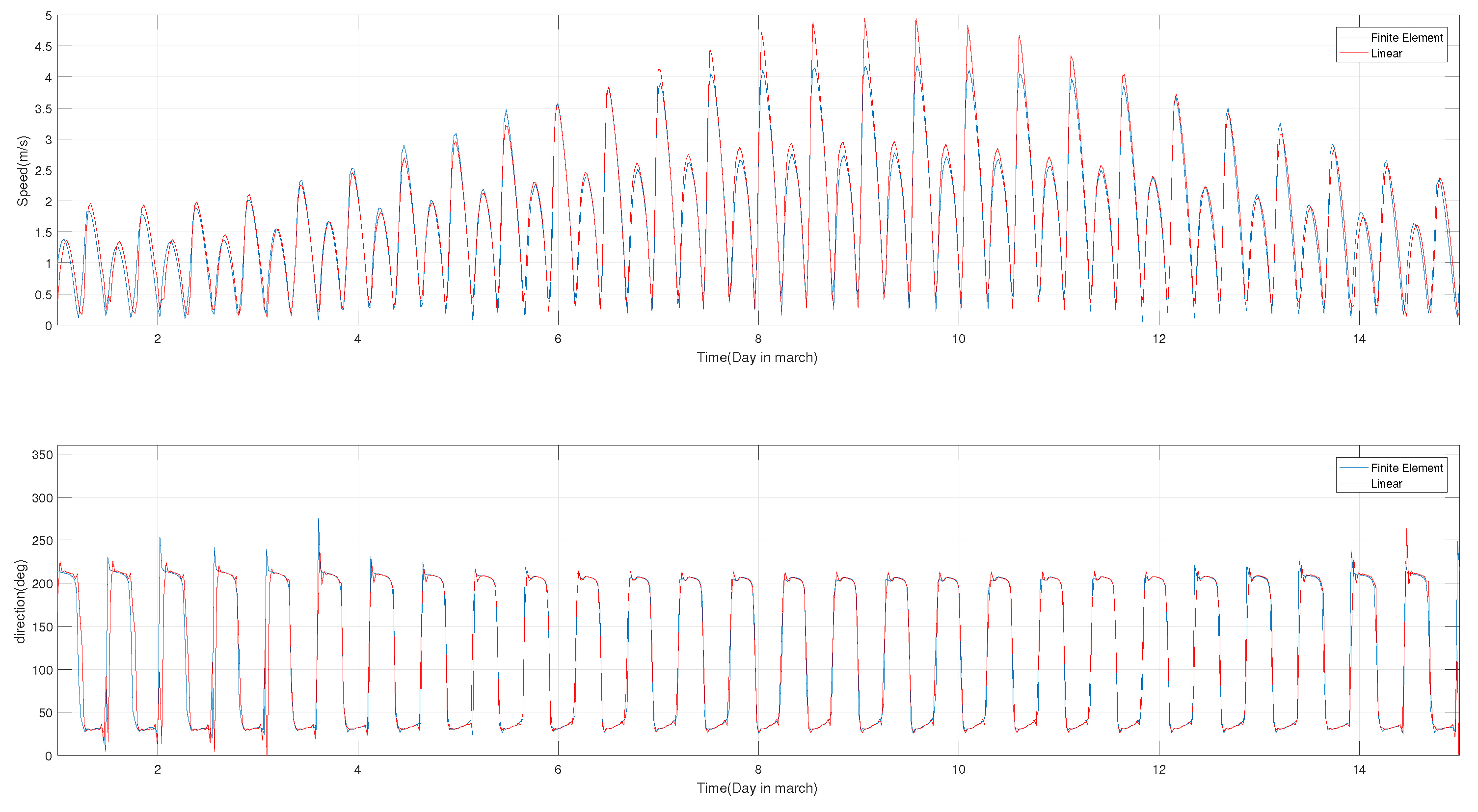
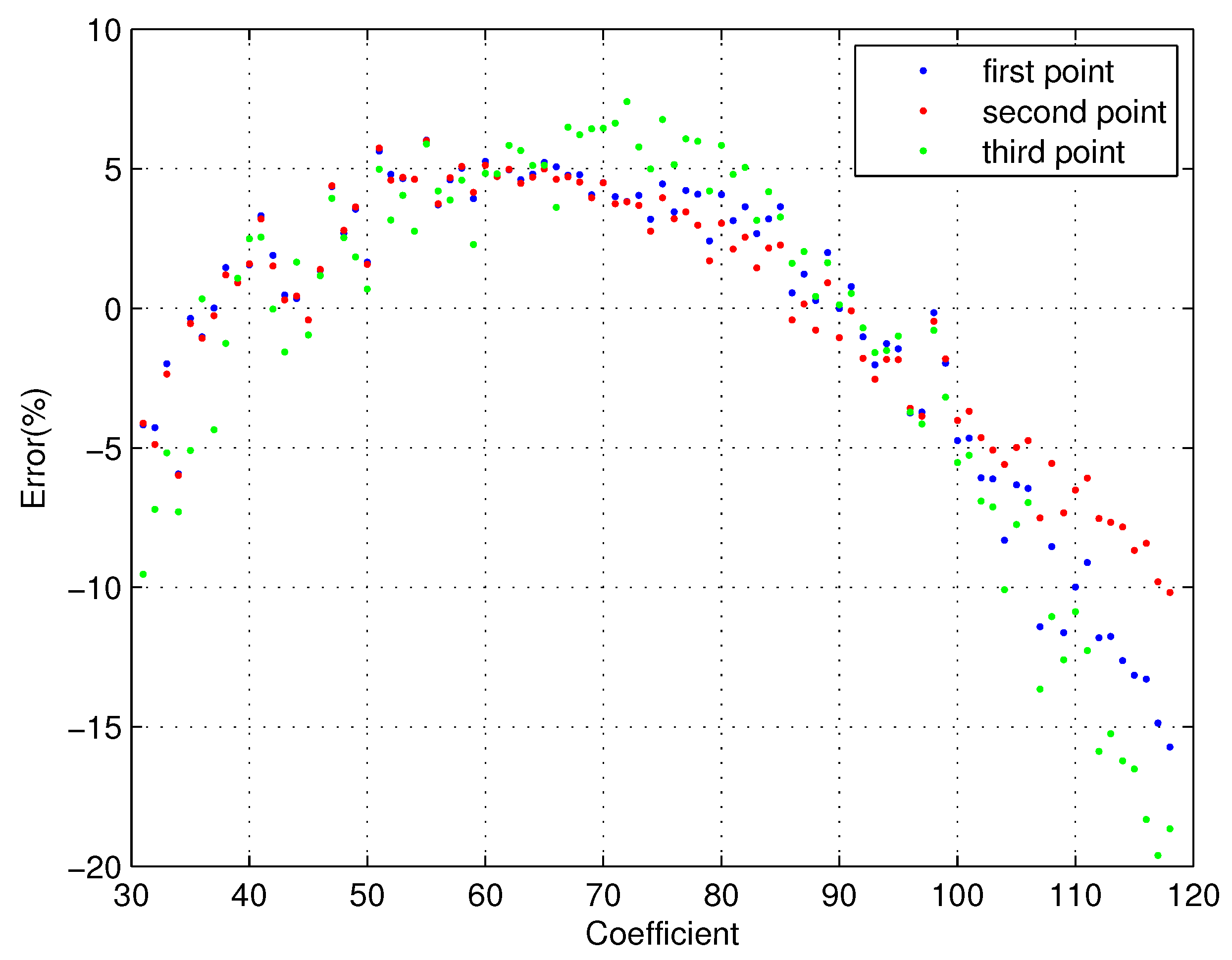
4.1. Current Time Series Prediction Comparison
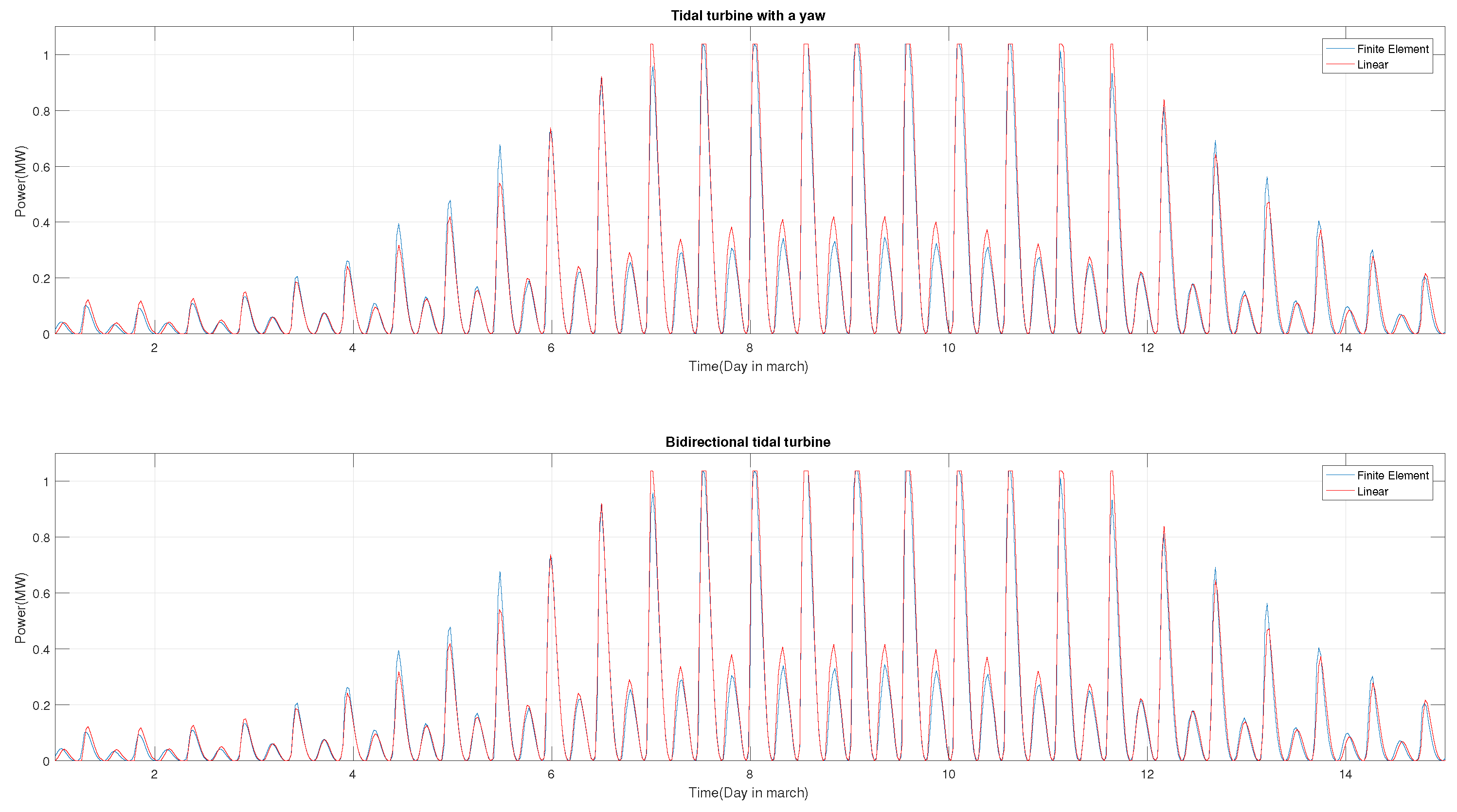
4.2. Energy Harnessing Comparison with Yawed and Fixed Axis Turbine
5. Conclusions
Author Contributions
Funding
Acknowledgments
Conflicts of Interest
References
- Maslov, N.; Charpentier, J.F.; Claramunt, C. A modelling approach for a cost-based evaluation of the energy produced by a marine energy farm. Int. J. Mar. Energy 2015, 9, 1–19. [Google Scholar] [CrossRef]
- El Tawil, T.; Charpentier, J.F.; Benbouzid, M. Tidal energy site characterization for marine turbine optimal installation: Case of the Ouessant Island in France. Int. J. Mar. Energy 2017, 18, 57–64. [Google Scholar] [CrossRef]
- Neill, S.; Hashemi, M.; Lewis, M. Tidal energy leasing and tidal phasing. Renew. Energy 2016, 85, 580–587. [Google Scholar] [CrossRef]
- Guillou, N.; Neill, S.P.; Robins, P.E. Characterising the tidal stream power resource around France using a high-resolution harmonic database. Renew. Energy 2018, 123, 706–718. [Google Scholar] [CrossRef]
- Zhou, Z.; Benbouzid, M.; Charpentier, J.F.; Scuiller, F.; Tang, T. Developments in large marine current turbine technologies—A review. Renew. Sustain. Energy Rev. 2017, 71, 852–858. [Google Scholar] [CrossRef]
- Guillou, N.; Chapalain, G. Tidal Turbines’ Layout in a Stream with Asymmetry and Misalignment. Energies 2017, 10, 1892. [Google Scholar] [CrossRef]
- Epler, J.; Polagye, B.; Thomson, J. Shipboard Acoustic Doppler Current Profiler Surveys to Assess Tidal Current Resources. In Proceedings of the IEEE OCEANS 2010, Sydney, Australia, 24–27 May 2010. [Google Scholar]
- Fairley, I.; Evans, P.; Wooldridge, C.; Willis, M.; Masters, I. Evaluation of tidal stream resource in a potential array via direct measurements. Renew. Energy 2013, 57, 70–78. [Google Scholar] [CrossRef]
- Carpmand, N.; Thomas, K. Tidal resource characterization in the Folda Fjord, Norway. Int. J. Mar. Energy 2016, 13, 27–44. [Google Scholar] [CrossRef]
- Hervouet, J.M. Hydrodynamics of Free Surface Flows: Modelling with the Finite Element Method; John Wiley & Sons: Hoboken, NJ, USA, 2007. [Google Scholar]
- Guillou, N.; Thiébot, J. The impact of seabed rock roughness on tidal stream power extraction. Energy 2016, 112, 762–773. [Google Scholar] [CrossRef]
- Guillou, N.; Chapalain, G.; Neill, S.P. The influence of waves on the tidal kinetic energy resource at a tidal stream energy site. Appl. Energy 2016, 180, 402–415. [Google Scholar] [CrossRef]
- SHOM. MNT Bathymétrique de la Façade Atlantique (Projet HOMONIM). Available online: http:// diffusion.shom.fr/produits/bathymetrie/mnt-facade-atl-homonim.html (accessed on 1 September 2017).
- Loubrieu, B.; Bourillet, J.; Moussat, E. Bathy-Morphologique Régionale du Golfe de Gascogne et de la Manche, Modèle Numérique; Technical Report; IFREMER: Issy-les-Moulineaux, France, 2008.
- Hamdi, A.; Vasquez, M.; Populus, J. Cartographie des Habitats Physiques Eunis-Côtes de France; Technical Report DYNECO/AG/10-26/JP; IFREMER: Issy-les-Moulineaux, France, 2010.
- Soulsby, R.L. The bottom boundary layer of shelf seas. In Elsevier Oceanography Series; Elsevier: Amsterdam, The Netherlands, 1983; Volume 35, pp. 189–266. [Google Scholar]
- Smagorinsky, J. General circulation experiments with the primitive equations. I: The basic experiments. Mon. Weather Rev. 1963, 91, 99–164. [Google Scholar] [CrossRef]
- Quetin, B. Modèles mathématiques de calcul des ećoulements induits par le vent. In Proceedings of the 17th Congress of the International Association of Hydraulic Research, Baden-Baden, Germany, 15–19 August 1977. [Google Scholar]
- Egbert, G.D.; Bennett, A.F.; Foreman, M.G. TOPEX/POSEIDON tides estimated using a global inverse model. J. Geophys. Res. Oceans 1994, 99, 24821–24852. [Google Scholar] [CrossRef]
- Simon, B. La marée La marée Océanique Côtière; Institut Océanographique: Paris, France, 2007; p. 435. [Google Scholar]
- SHOM. Service Hydrographique et Océanographique de la Marine (2016). Courants de Marée—Mer d’Iroise de L’île Vierge à la Pointe de Penmarc’h; Technical report 560-UJA; SHOM: Brest, France, 2016.
- SHOM. Available online: http://maree.info/82/calendrier (accessed on 5 September 2018).
- Ajiwibowo, H.; Lodiwa, K.S.; Pratama, M.B.; Wurjanto, A. Field measurement and numerical modeling of tidal current in Larantuka Strait for renewable energy utilization. Int. J. Geomate 2017, 13, 124–131. [Google Scholar] [CrossRef]
- Zhou, Z.; Scuiller, F.; Charpentier, J.F.; Benbouzid, M.E.H.; Tang, T. Power control of a nonpitchable PMSG-based marine current turbine at overrated current speed with flux-weakening strategy. IEEE J. Ocean. Eng. 2015, 40, 536–545. [Google Scholar] [CrossRef]
- Arnold, M.; Biskup, F.; Cheng, P.W. Load reduction potential of variable speed control approaches for fixed pitch tidal current turbines. Int. J. Mar. Energy 2016, 15, 175–190. [Google Scholar] [CrossRef]


| Locations | Longitude | Latitude | Mean Water Depths |
|---|---|---|---|
| # 1 | W | N | 58 m |
| # 2 | W | N | 56 m |
| # 3 | W | N | 54 m |
| Turbine diameter | 10 m |
| Turbine power coefficient | 0.4 |
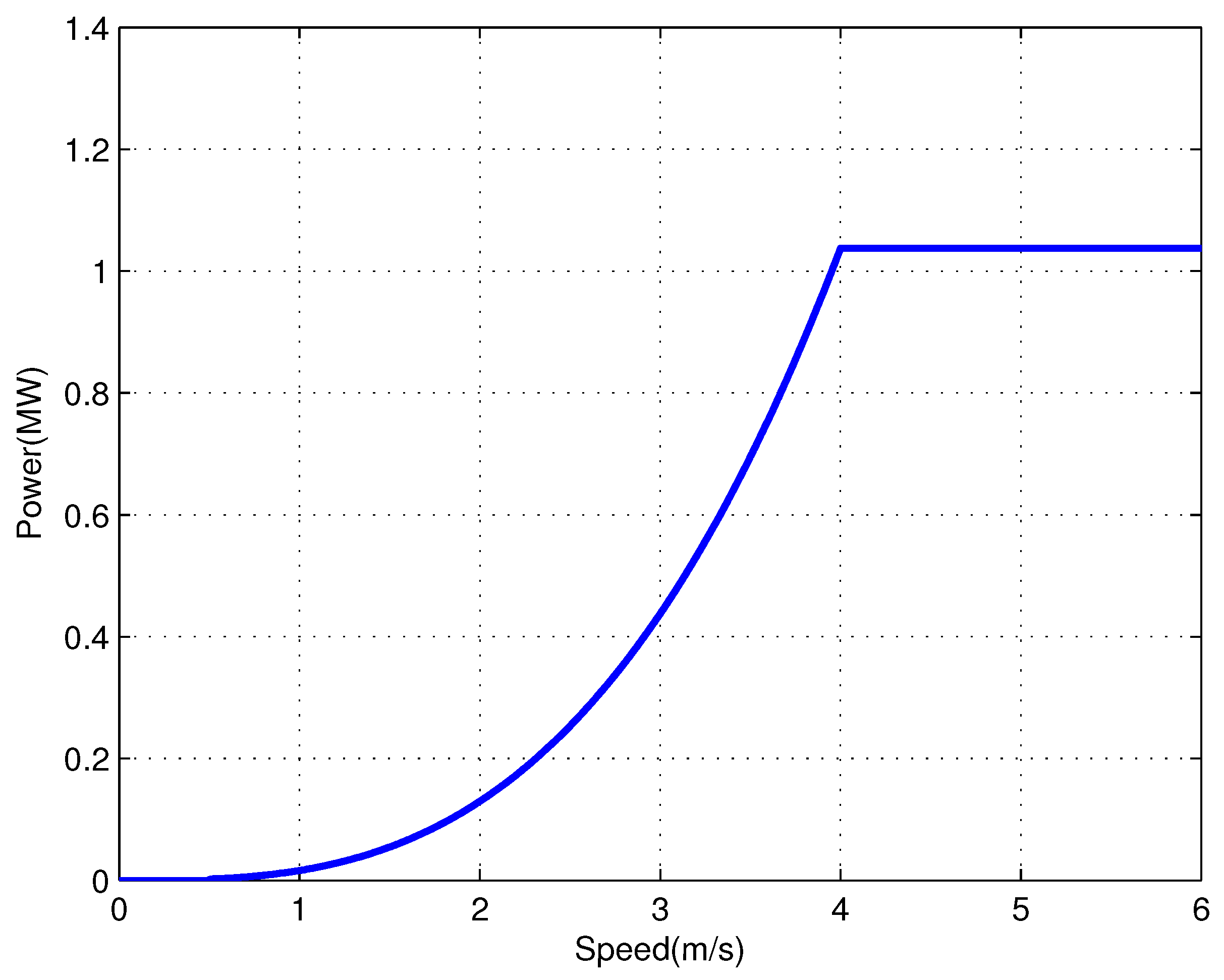
| Cut-in speed | 0.5 m/s |
| Nominal speed | 4 m/s |
| Nominal power | 1 MW |
| Detailed Method | Linear Approximation Method | |||||
|---|---|---|---|---|---|---|
| Yawed | Fixed Axis | Difference (%) | Yawed | Fixed Axis | Difference (%) | |
| #1 | 1193 | 1190 | 0.25 | 1213.6 | 1204 | 0.79 |
| #2 | 1275 | 1262 | 0.99 | 1296.9 | 1285 | 0.89 |
| #3 | 1283 | 1278 | 0.37 | 1281.3 | 1275 | 0.44 |
© 2019 by the authors. Licensee MDPI, Basel, Switzerland. This article is an open access article distributed under the terms and conditions of the Creative Commons Attribution (CC BY) license (http://creativecommons.org/licenses/by/4.0/).
Share and Cite
El Tawil, T.; Guillou, N.; Charpentier, J.-F.; Benbouzid, M. On Tidal Current Velocity Vector Time Series Prediction: A Comparative Study for a French High Tidal Energy Potential Site. J. Mar. Sci. Eng. 2019, 7, 46. https://doi.org/10.3390/jmse7020046
El Tawil T, Guillou N, Charpentier J-F, Benbouzid M. On Tidal Current Velocity Vector Time Series Prediction: A Comparative Study for a French High Tidal Energy Potential Site. Journal of Marine Science and Engineering. 2019; 7(2):46. https://doi.org/10.3390/jmse7020046
Chicago/Turabian StyleEl Tawil, Tony, Nicolas Guillou, Jean-Frédéric Charpentier, and Mohamed Benbouzid. 2019. "On Tidal Current Velocity Vector Time Series Prediction: A Comparative Study for a French High Tidal Energy Potential Site" Journal of Marine Science and Engineering 7, no. 2: 46. https://doi.org/10.3390/jmse7020046
APA StyleEl Tawil, T., Guillou, N., Charpentier, J.-F., & Benbouzid, M. (2019). On Tidal Current Velocity Vector Time Series Prediction: A Comparative Study for a French High Tidal Energy Potential Site. Journal of Marine Science and Engineering, 7(2), 46. https://doi.org/10.3390/jmse7020046