Detection of Visual Signatures of Marine Mammals and Fish within Marine Renewable Energy Farms using Multibeam Imaging Sonar


Abstract
1. Introduction
2. Methods
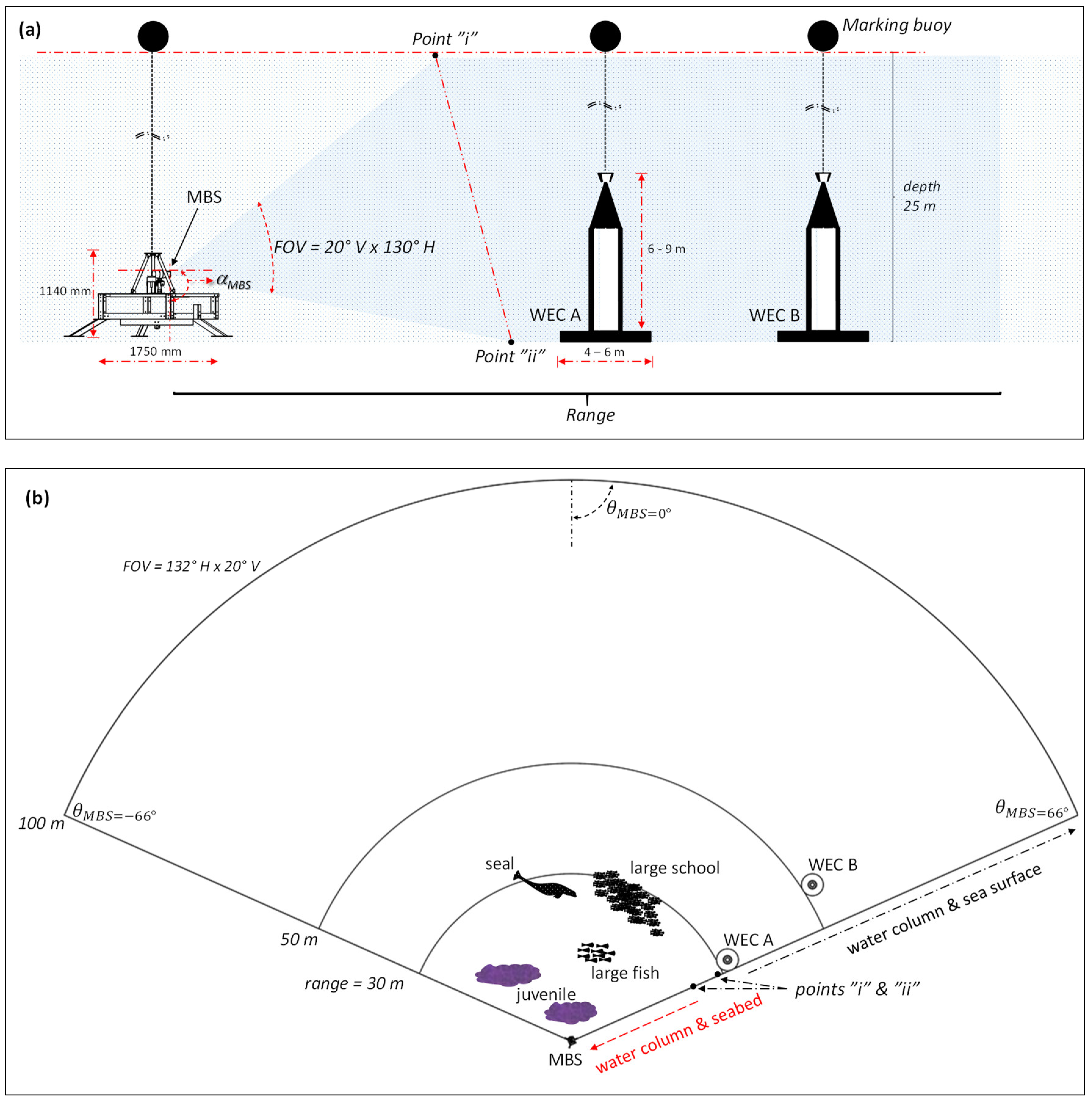
2.1. Survey Design
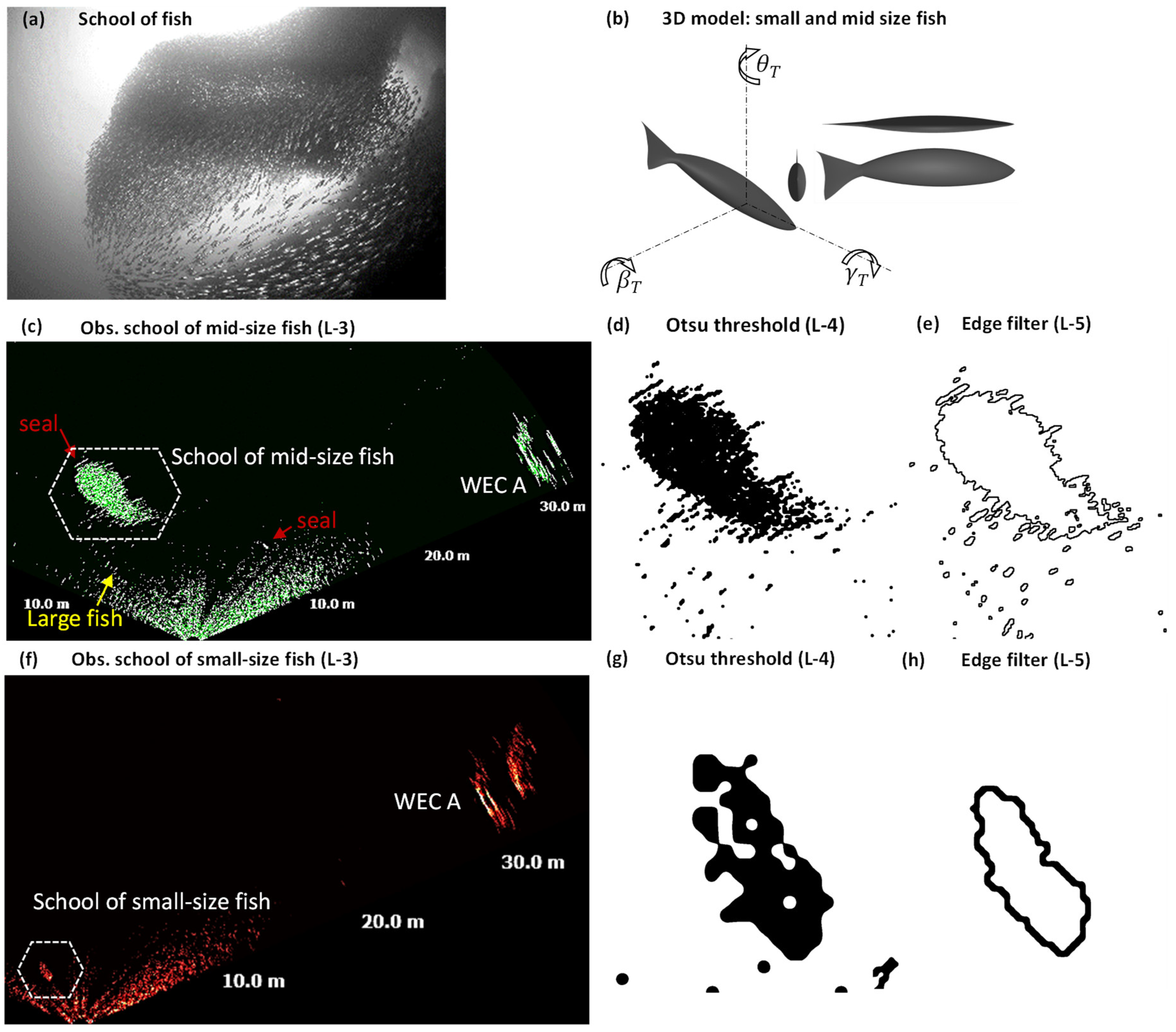
2.2. Data processing Protocol
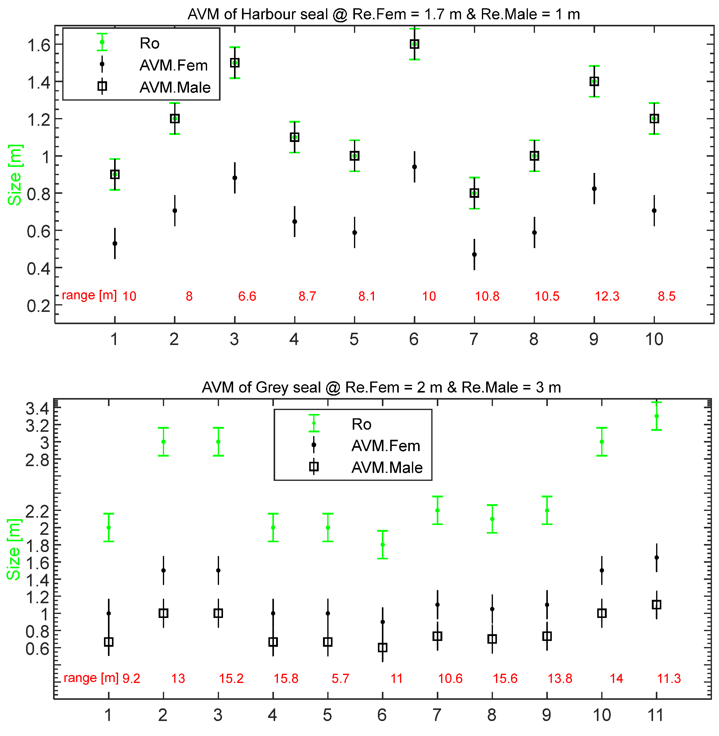
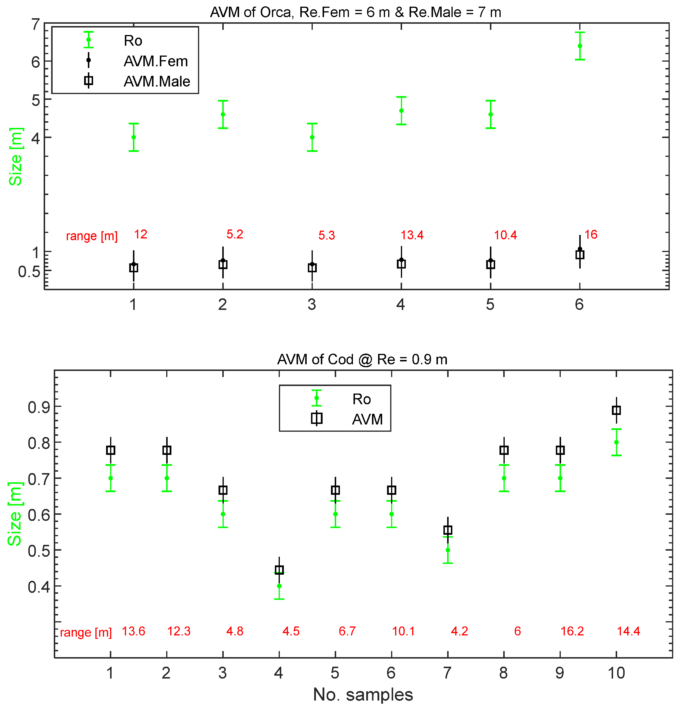
2.3. The Acoustic Visibility Measure
3. Results and Discussion
3.1. Schools of Fish
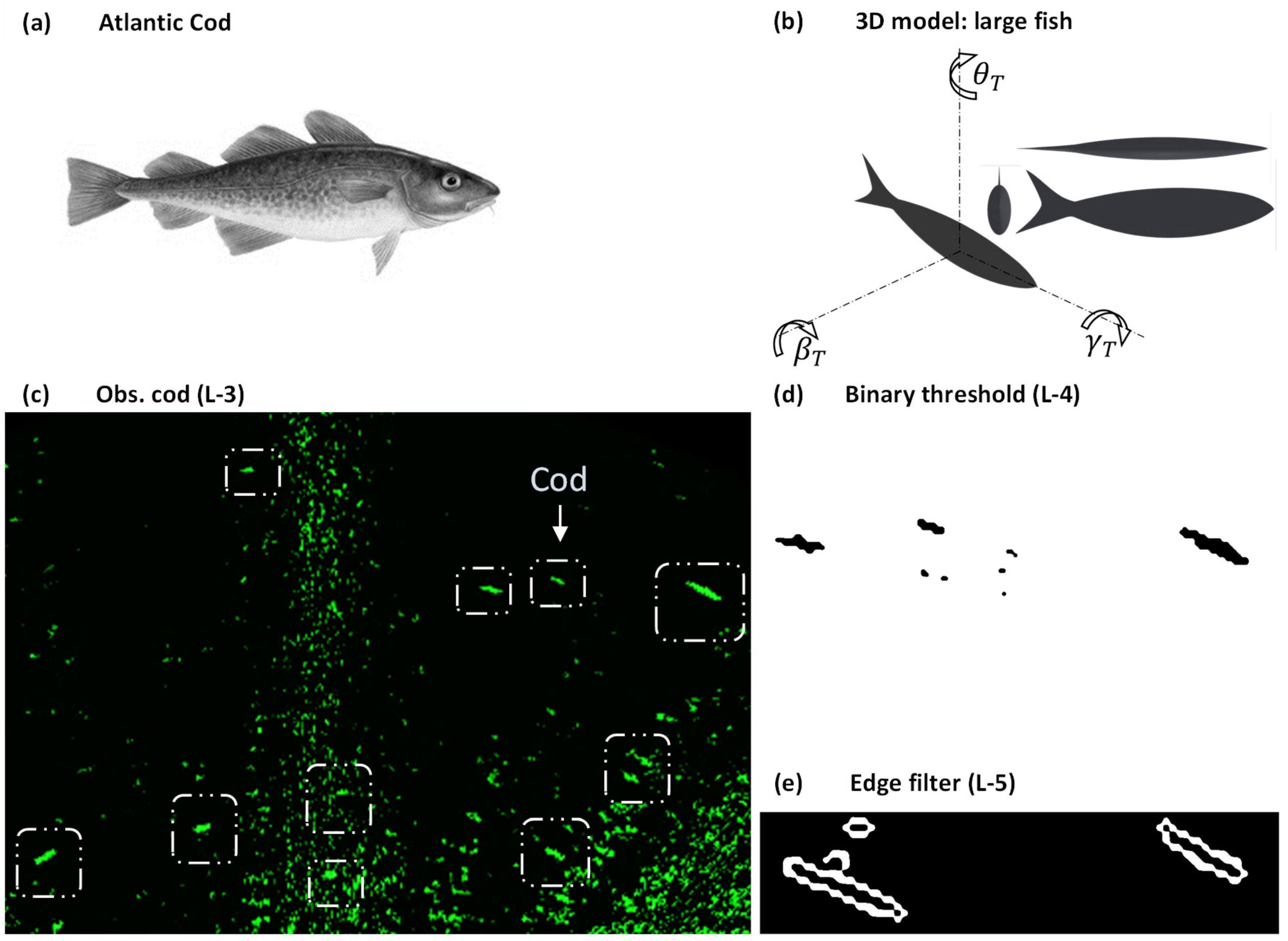
3.2. Large Fish
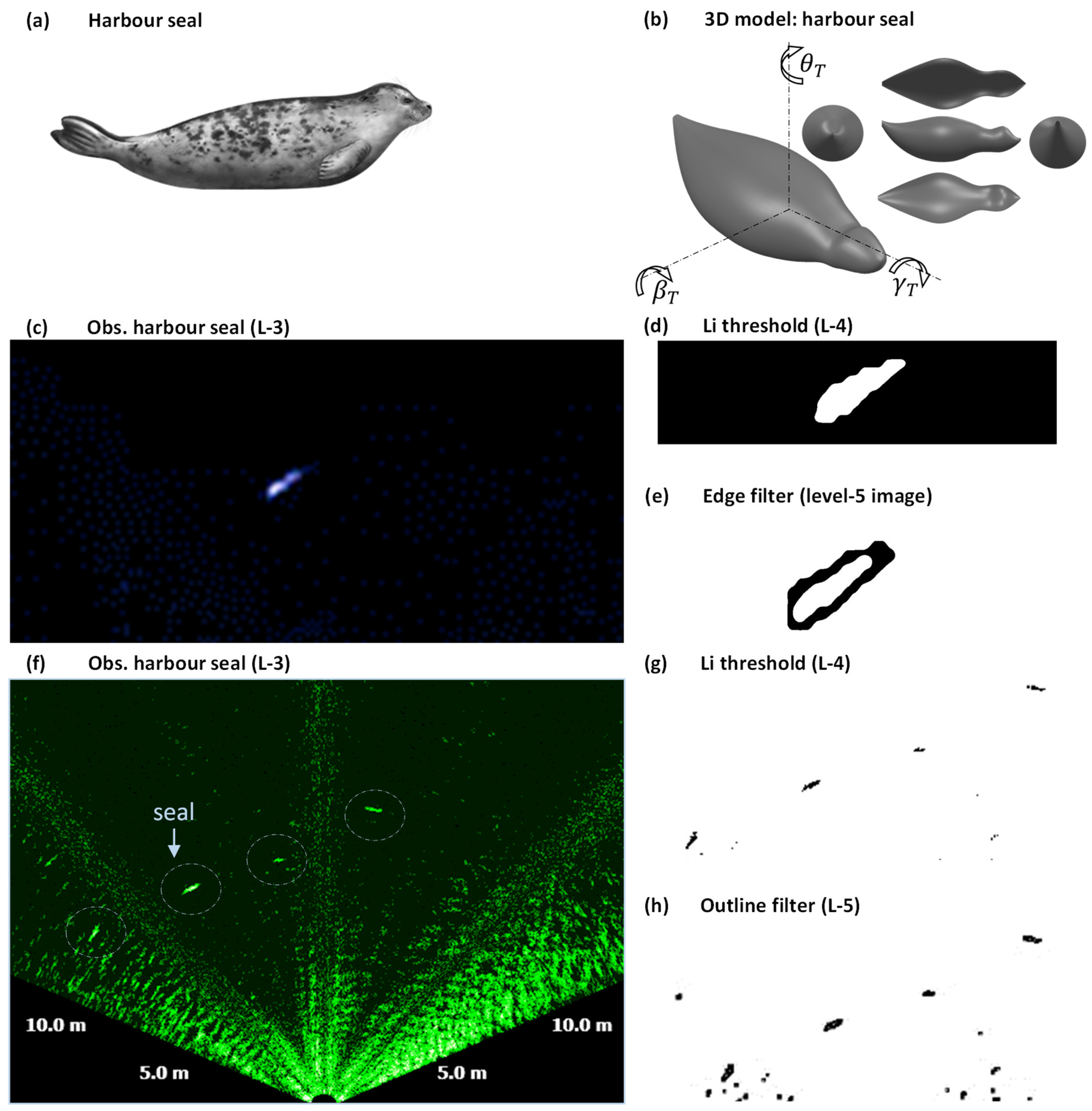
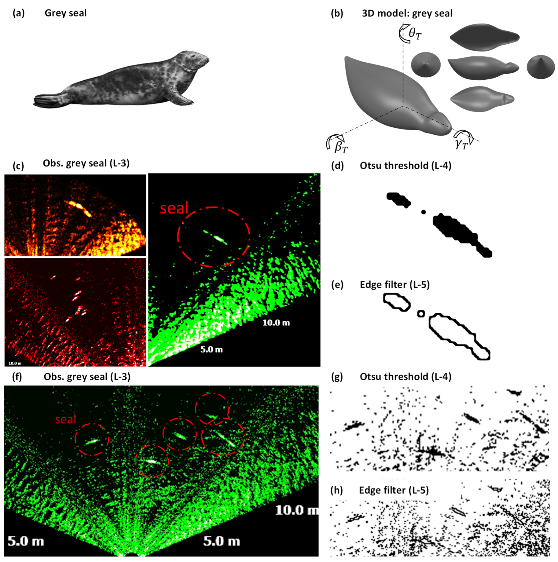
3.3. Seals
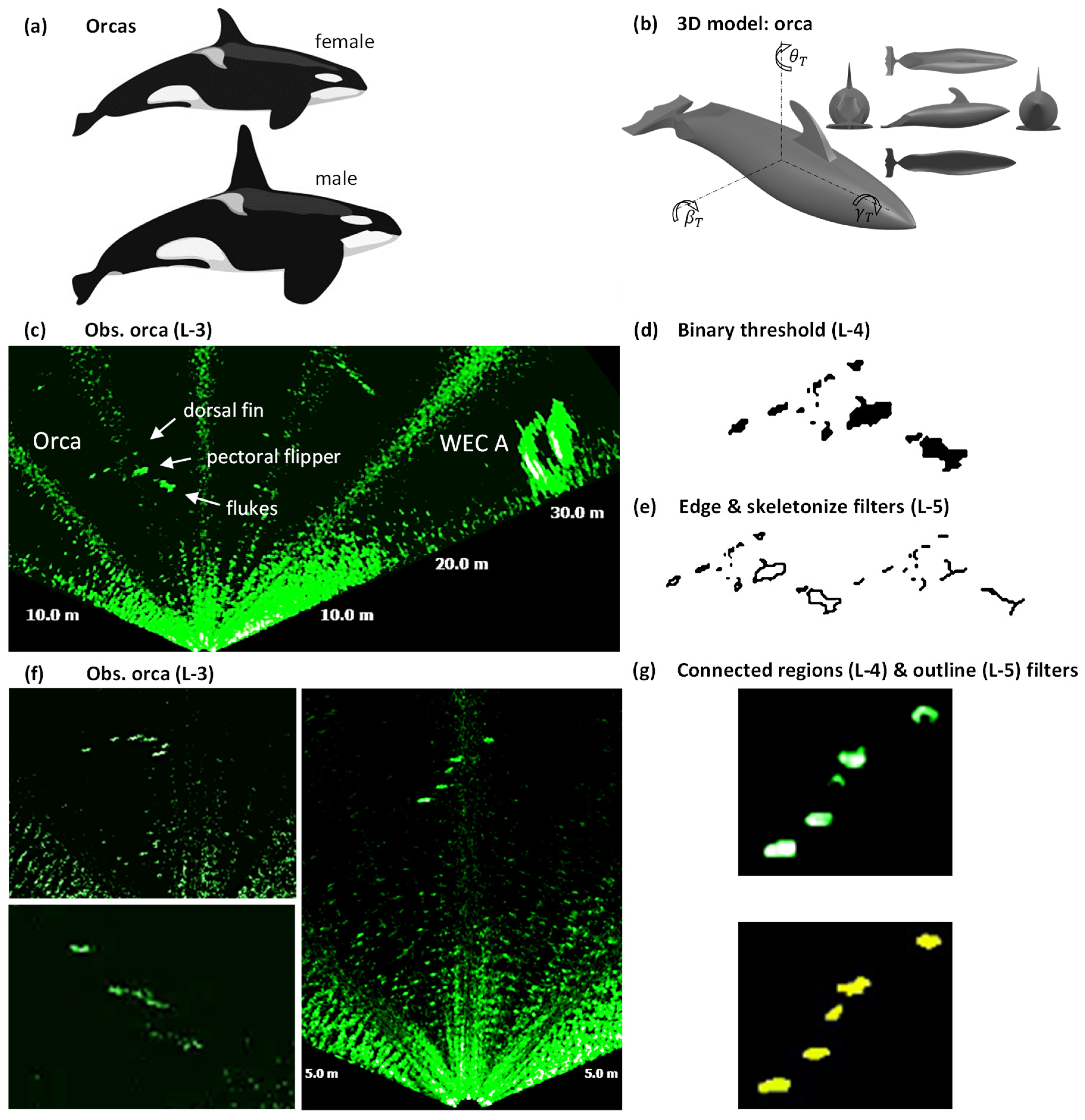
3.4. Orcas
3.5. Combined Occurrence of Different Targets
4. Conclusions
Author Contributions
Funding
Conflicts of Interest
References
- Wilson, B.; Batty, R.S.; Daunt, F.; Carter, C. Collision risks between marine renewable energy devices and mammals, fish and diving birds. In Report to the Scottish Executive. Scottish Association for Marine Science; Scottish Association for Marine Science: Oban, Scotland, 2007; pp. 1–110. [Google Scholar]
- Boehlert, G.W.; Gill, A.B. Environmental and ecological effects of ocean renewable energy development: A current synthesis. Oceanography 2010, 23, 68–81. [Google Scholar] [CrossRef]
- Ward, E.H.R.D.; Sawyer, T.C. Environmental Assessment, Management and Monitoring of Carnegie Wave Energy’s Perth Wave Energy Project. In Proceedings of the 11th European Wave and Tidal Energy Conference, Nante, France, 6–11 September 2015. [Google Scholar]
- Francisco, F.; Sundberg, J. Sonar for environmental monitoring. Initial setup of an active acoustic platform. In Proceedings of the International Offshore and Polar Engineering Conference, Maui, HI, USA, 21–26 June 2015. [Google Scholar]
- Francisco, F.; Sundberg, J.; Leijon, M. Sonar for Environmental Monitoring: Understanding the Functionality of Active Acoustics as a Method for Monitoring Marine Renewable Energy Devices. In Proceedings of the 11th European Wave and Tidal Energy Conference, Nantes, France, 6–11 September 2015. [Google Scholar]
- Bender, A.; Francisco, F.G.A.; Sundberg, J. A Review of Methods and Models for Environmental Monitoring of Marine Renewable Energy. In Proceedings of the 12th European Wave and Tidal Energy Conference, Cork, Ireland, 27th August–1 September 2017. [Google Scholar]
- Geoffroy, M.; Knudsen, F.R.; Fortier, L. Target strengths and echotraces of whales and seals in the Canadian Beaufort Sea. ICES J. Mar. Sci. 2015, 73, 451–463. [Google Scholar] [CrossRef]
- Kerrie, P.; Mark, J.; David, B.; Peter, A. Using dual-frequency identification sonar (DIDSON) to estimate adult steelhead escapement in the San Lorenzo river, California. Calif. Fish Game 2010, 96, 90–95. [Google Scholar]
- Francisco, F.; Sundberg, J. Sonar for Environmental Monitoring: Configuration of a Multifunctional Active Acoustics Platform Applied for Marine Renewables. Unpublished work. 2016. [Google Scholar]
- Williamson, B.J.; Blondel, P.; Armstrong, E.; Bell, P.S.; Hall, C.; Waggitt, J.J.; Scott, B.E. A Self-Contained Subsea Platform for Acoustic Monitoring of the Environment Around Marine Renewable Energy Devices-Field Deployments at Wave and Tidal Energy Sites in Orkney, Scotland. IEEE J. Ocean. Eng. 2016, 41, 67–81. [Google Scholar]
- Sparling, C.; Gillespie, D.; Hastie, G.; Gordon, J.; Macaulay, J.; Malinka, C.; Wu, M.; Mcconnell, B. Scottish Government Demonstration Strategy: Trialling Methods for Tracking the Fine Scale Underwater Movements of Marine Mammals in Areas of Marine Renewable Energy Development. Scott. Mar. Freshw. Sci. 2016, 7, 114. [Google Scholar]
- Bevelhimer, M.; Colby, J.; Adonizio, M.A.; Tomichek, C.; Scherelis, C.S. Informing a Tidal Turbine Strike Probability Model through Characterization of Fish Behavioral Response Using Multibeam Sonar Output; Oak Ridge National Laboratory: Oak Ridge, TN, USA, 2016. [Google Scholar]
- Marine Energy, EMEC: European Marine Energy Centre. Available online: http://www.emec.org.uk/marine-energy/ (accessed on 1 October 2018).
- Available online: http://fundyforce.ca/environment/enviromental-assesment/ (accessed on 1 October 2018).
- Langhamer, O. Effects of wave energy converters on the surrounding soft-bottom macrofauna (west coast of Sweden). Mar. Environ. Res. 2010, 69, 374–381. [Google Scholar] [CrossRef]
- Langhamer, O.; Haikonen, K.; Sundberg, J. Wave power-Sustainable energy or environmentally costly? A review with special emphasis on linear wave energy converters. Renew. Sustain. Energy Rev. 2010, 14, 1329–1335. [Google Scholar] [CrossRef]
- Haikonen, K.; Sundberg, J.; Leijon, M. Characteristics of the operational noise from full scale wave energy converters in the Lysekil project: Estimation of potential environmental impacts. Energies 2013, 6, 2562–2582. [Google Scholar] [CrossRef]
- Grear, M.; Motley, M. Tidal turbine collision assessment using the bulk and shear modulus of marine mammals’ soft tissue. In Proceedings of the Twelfth European Wave and Tidal Energy Conference, Cork, Ireland, 27th August–1 September 2017. [Google Scholar]
- Hammar, L. Power from the Brave New Ocean: Marine Renewable Energy and Ecological Risks. Ph.D. dissertation, Chalmers University of Technology, Gothenburg, Sweden, 2014; p. 67. [Google Scholar]
- Hovem, J.M. Underwater acoustics: Propagation, devices and systems. J. Electroceram. 2007, 19, 339–347. [Google Scholar] [CrossRef]
- Mcgehee, D.; Jaffe, J.S. Three-dimensional swimming behavior of individual zooplankters: observations using the acoustical imaging system FishTV. ICES J. Mar. Sci. 1996, 53, 363–369. [Google Scholar] [CrossRef]
- Waite, A.D. Sonar for Practising Engineers; John Wiley & Sons Ltd.: Hoboken, NJ, USA, 2002; ISBN 0 471 49750 9. [Google Scholar]
- Chu, D. Technology evolution and advances in fisheries acoustics. J. Mar. Sci. Technol. 2011, 19, 245–252. [Google Scholar]
- Parwal, A.; Remouit, F.; Hong, Y.; Francisco, F.; Castelucci, V.; Hai, L.; Ulvgård, L.; Li, W.; Lejerskog, E.; Baudoin, A.; et al. Wave Energy Research at Uppsala University and The Lysekil Research Site, Sweden: A Status Update. In Proceedings of the 11th European Wave and Tidal Energy Conference, Nantes, France, 6–11 September 2015. [Google Scholar]
- Teledyne PDS. Available online: http://www.teledyne-pds.com/ (accessed on 1 October 2018).
- Schindelin, J.; Arganda-Carreras, I.; Frise, E.; Kaynig, V.; Longair, M.; Pietzsch, T.; Preibisch, S.; Rueden, C.; Saalfeld, S.; Schmid, B.; et al. Fiji: An open-source platform for biological-image analysis. Nat. Methods 2012, 9, 676. [Google Scholar] [CrossRef] [PubMed]
- Priya, M.S.; Nawaz, G.M.K. Multilevel Image Thresholding using OTSU’s Algorithm in Image Segmentation. Int. J. Sci. Eng. Res. 2017, 8, 101–106. [Google Scholar]
- Stål, J.; Paulsen, S.; Pihl, L.; Rönnbäck, P.; Söderqvist, T. Coastal Habitat Support to Fish and Fisheries on the Swedish West Coast; Department of Marine Ecology, Göteborg University, Kristineberg Marine Research Station: Fiskebäckskil, Sweden, 2007; pp. 1–17. [Google Scholar]
- Pihl, L.; Rosenberg, R. Production, abundance, and biomass of mobile epibenthic marine fauna in shallow waters, Western Sweden. J. Exp. Mar. Bio. Ecol. 1982, 57, 273–301. [Google Scholar] [CrossRef]
- Almesj, L.; Lim, H. Fish Populations in Swedish Waters: How Are They Influenced by Fishing, Eutrophication and Contaminants? The Riksdag Printing Office: Stockholm, Sweden, 2009; p. 80. [Google Scholar]
- Chudzinska, M. Diving behaviour of harbour seals (Phoca vitulina) from the Kattegat. Master’s thesis, Department of Arctic Environment, National Environmental Research Institute, University of Aarhus, Denmark, Aarhus, 2009; p. 69. [Google Scholar]
- Härkönen, T.; Harding, K.C. Spatial structure of harbour seal populations and the implications thereof. Can. J. Zool. 2001, 79, 2115–2127. [Google Scholar] [CrossRef]
- Solberg, I. Behavior and Ecology of Overwintering Sprat Sprattus Sprattus 2017. PhD dissertation, Faculty of Mathematics and Natural Sciences, University of Oslo, Oslo, Sweden, 2017. [Google Scholar]
- Global Biodiversity Information Facility GBIF-Sweden. 2018. Available online: http://www.gbif.se/portal/#/index (accessed on 1 September 2018).
- HELCOM (Baltic Marine Environment Protection Commission—Helsinki Commission). 2018. Available online: http://maps.helcom.fi/website/mapservice/index.html (accessed on 1 September 2018).
- Cod (Gadus Morhua). European Commission, 2018. Available online: https://ec.europa.eu/fisheries/marine_species/wild_species/cod_en (accessed on 20 August 2008).
- Lesage, V.; Hammill, M.O.; Kovacs, K.M. Functional classification of harbor seal (Phoca vitulina) dives using depth profiles, swimming velocity, and an index of foraging success. Can. J. Zool. 1999, 77, 74–87. [Google Scholar] [CrossRef]
- Killer Whales: Physical Characteristics. SeaWorld Parks & Entertainment, 2018. Available online: https://seaworld.org/animal-info/animal-infobooks/killer-whale/physical-characteristics/ (accessed on 20 August 2011).
- Uppsala University Publications. DiVA portal: Francisco, Francisco. Available online: http://uu.diva-portal.org/smash/person.jsf?pid=authority-person:21725 (accessed on 1 December 2018).
- Francisco, F.; Bender, A.; Sundberg, J. Use of Multibeam Imaging Sonar for Observation of Marine Mammals and Fish on a Marine Renewable Energy Site. Unpublished work. 2018. [Google Scholar]
- Hastie, G.D.; Donovan, C.; Götz, T.; Janik, V.M. Behavioral responses by grey seals (Halichoerus grypus) to high frequency sonar. Mar. Pollut. Bull. 2014, 79, 205–210. [Google Scholar] [CrossRef]
- Hammond, P.S.; Nicholas, K.S.; Fepak, M.A.; Mammal, S.; Antarctic, B.; Cross, H.; Road, M. Movements, diving and foraging behaviour of grey seals. 1991, 224, 223–232. [Google Scholar]
- Jefferson, T.A.; Leatherwood, S.; Webber, M.A. Marine Mammals of the World; United Nations Environment Programme: Washington DC, USA, 1993; ISBN 9251032920. [Google Scholar]
- Königson, S. Seal behaviour around fishing gear and its impact on Swedish fisheries. Ph.D. thesis, Department of Marine Ecology, Swedish Board of Fisheries, Göteborg University, Göteborg, Sweden, 2007; p. 20. [Google Scholar]
- William, F. Perrin; Würsig, B.; Thewissen, J.G.M. Encyclopedia of Marine Mammals, 3rd ed.; Academic Press: San Diego, CA, USA, 2017; ISBN 987-0-12-373553-9. [Google Scholar]
- Atlantic Cod: Gadus Morhua Linnaeus. Global Biodiversity Information Facility, 2018. Available online: https://www.gbif.org/species/113235764 (accessed on 20 August 2008).
- Combourieu, A.; Lawson, M.; Babarit, A.; Ruehl, K.; Roy, A.; Costello, R.; Weywada, P.L.; Bailey, H. WEC3: Wave Energy Converter Code Comparison Project. In Proceedings of the 11th European Wave and Tidal Energy Conference, Nantes, France, 6–11 September 2015. [Google Scholar]
- Francisco, F.; Sundberg, J. Evaluation of Underwater Acoustic and Optical Imaging for Structural Inspections for Marine Renewables. Unpublished work. 2018. [Google Scholar]
- Francisco, F.; Carpman, N.; Dolguntseva, I.; Sundberg, J. Use of Multibeam and Dual-Beam Sonar Systems to Observe Cavitating Flow Produced by Ferryboats: In a Marine Renewable Energy Perspective. J. Mar. Sci. Eng. 2017, 5, 1–15. [Google Scholar] [CrossRef]


| Component | Specification |
|---|---|
| MBS BlueView M900-130-S-MKS-VSDL | Frequency: 0.9 MHz (operational) Number of Beams: 768 Refresh rate: up to 50 Hz (sample frequency) FOV: 132° × 20° (field of view) Resolution: 0.18° / 2.54 cm Maximum range: 100 m |
| ProViwer4 | Sound speed:1500 m/s | 1527 m/s Sensitivity: 19.9 dB | 29.4dB Intensity: 90 dB | 95.9 dB Gama: 0.5 | 1.2 | Levels 2 | 3 images |
| FIJI-ImageJ2 | Threshold and filters: - 8 | 32 bit binary - Outline | Edges | Skeletonize - Connected regions | Level 4 images Level 5 images Level 5 images |
| Solidworks2013 | - Building of 3-D models - Reconstruction of shape and size | Level 6 images |
| Animal (Spp) | Size | Animal (Spp) | Size |
|---|---|---|---|
| Atlantic cod (Gadus morhua) | 60 cm–1.2 m | Grey seal (Halichoerus grypus) | Males 2–3.3 m, avg. 2m; Females 1.6–2 m, avg. 1.8 m |
| Atlantic herring (Clupea harengus) | 24–45 cm | Harbour seal (Phoca vitulina) | Males avg. 1.7 m; Female avg. 1 m |
| European sprat (Sprattus sprattus) | 8–16 cm | Orca (Orcinus orca) | Males 6–8 m; Females 5–7 m; Dorsal fin 0.9–1.8 m |
| Northeast Atlantic mackerel (Scomber scombrus) | 30–66 cm |
| Class | Harbour Seal | Grey Seal | Orca | Small Fish | Medium Fish | Cod |
|---|---|---|---|---|---|---|
| Observed length | 1–2 m | 2–4 m | >4 m | <20 cm | <40 cm | >40 cm |
| Approximated geometric shape | ellipsoidal | ellipsoidal-bulkier | ellipsoidal streamlined-bulkier | ellipsoidal | ellipsoidal | ellipsoidal-bulkier |
| Observed swimming behavior | slow–fast | slow–fast | fast | slow–fast | fast | static–slow |
© 2019 by the authors. Licensee MDPI, Basel, Switzerland. This article is an open access article distributed under the terms and conditions of the Creative Commons Attribution (CC BY) license (http://creativecommons.org/licenses/by/4.0/).
Share and Cite
Francisco, F.; Sundberg, J. Detection of Visual Signatures of Marine Mammals and Fish within Marine Renewable Energy Farms using Multibeam Imaging Sonar. J. Mar. Sci. Eng. 2019, 7, 22. https://doi.org/10.3390/jmse7020022
Francisco F, Sundberg J. Detection of Visual Signatures of Marine Mammals and Fish within Marine Renewable Energy Farms using Multibeam Imaging Sonar. Journal of Marine Science and Engineering. 2019; 7(2):22. https://doi.org/10.3390/jmse7020022
Chicago/Turabian StyleFrancisco, Francisco, and Jan Sundberg. 2019. "Detection of Visual Signatures of Marine Mammals and Fish within Marine Renewable Energy Farms using Multibeam Imaging Sonar" Journal of Marine Science and Engineering 7, no. 2: 22. https://doi.org/10.3390/jmse7020022
APA StyleFrancisco, F., & Sundberg, J. (2019). Detection of Visual Signatures of Marine Mammals and Fish within Marine Renewable Energy Farms using Multibeam Imaging Sonar. Journal of Marine Science and Engineering, 7(2), 22. https://doi.org/10.3390/jmse7020022