System Modeling and Simulation of an Unmanned Aerial Underwater Vehicle

Abstract

Unmanned Aerial Underwater Vehicles (UAUVs) with multiple propellers can operate in two distinct mediums, air and underwater, and the system modeling of the autonomous vehicles is a key issue to adapt to these different external environments. In this paper, only a single set of aerial rotors with switching propulsion abilities are designed as driving components, and then a compound multi-model method is investigated to achieve good performance of the cross-medium motion. Furthermore, some additional variables, such as water resistance, buoyancy and their corresponding moments are considered for the underwater case. In particular, a critical coefficient for air-to-water switching is presented to express these gradually changing additional variables in the cross-medium motion process. Finally, the sliding mode control method is used to reduce the altitude error and attitude error of the vehicles with external environmental disturbances. The proposed scheme is tested and the model is verified on the simulation platform.

1. Introduction

Autonomous unmanned systems are very popular all over the world due to their broad range of applications such as surveillance, inspection, fast delivery, search and rescue, among many others [1,2,3]. In recent years, the rapid development of composite materials and the continuous upgrading of intelligent control technology have been of great help in the development of unmanned aerial vehicles (UAVs) and unmanned underwater vehicles (UUVs) [4,5]. More challenging, the unmanned aerial underwater vehicle (UAUV) has become a novel research field, which aims to design equipment that can fly in the air and navigate underwater. To enhance the characteristics of these unmanned systems, many scholars and enterprises have done lots of relevant work in fuselage shape, fuselage material, wing layout, mass-volume ratio, power system design, controller design and their intelligent applications and so on [6,7,8,9].

The system modeling and control of UAVs are investigated in some works. Many kinds of UAVs, such as fixed-wing, multi-rotor wing and flapping wing, have been developed and analyzed about their different structures and mathematical description method [10,11], and a lot of achievements have been made. Compared with traditional air vehicles, the control of multi-rotor vehicles are more stable and efficient. Thus, the multi-rotor vehicles have significant advantages in vertical take-off and landing (VTOL), precise hovering and aggressive maneuvers. In addition, transition flight modeling of a fixed-wing VTOL UAV is also investigated, and the model is specifically tailored for the design of a hover to forward flight and forward flight to hover transition control system [12]. Currently, there is no well accepted generic methodology that can be used for system modeling due to the fact that there are numerous challenges regarding the various configurations [13].

In addition, the system dynamics of UUVs has also been paid increasing attention by researchers. With the development of modern marine researches, many intelligent marine equipment, such as surface ships, semi-submarines, unmanned submarines and deep-sea robots, have been developed in all aspects. In particular, the underwater autonomous vehicles are facing unknown and hazardous environments, and their research and deployment have been regarded as one of significant goals and challenges by human beings. Therefore, an UUV with autonomous control should have capability to perceive its own position as well as its environment and react to unexpected or dynamic circumstances properly [14,15]. In addition, the system models of different shape configurations, such as open structure, torpedo-like and multi-thruster, are studied respectively [16,17]. Thruster fault detection and the isolation method and switching control of multi-thruster have been discussed [18,19].

UAVs and UUVs have broadened the space of operation from land to air or underwater, but both can still run only in a single medium. Unlike these unmanned systems, the UAUVs have attracted much attention and the existing literature mainly focuses on the mechanical structure design and cross-medium control [20,21]. The work in [22] focused on the modeling and trajectory tracking control of a special class of air-underwater vehicles with full torque actuation and a single thrust force directed along the vehicle’s vertical axis. Furthermore, the work in [23] presented a robust switching control for stabilizing the attitude of a hybrid UAUV, and discussed the effects of buoyancy force and added inertia. A hybrid controller was designed for trajectory tracking considering the full system, including a transition strategy to assure switching between mediums. Stability analysis for the full system was provided using hybrid Lyapunov and invariance principles [24]. Based on the adaptation of typical platforms for aerial and underwater vehicles, the architecture for this kind of quadrotor-like vehicle was evaluated to allow the navigation in both environments [25].

At present, there are still many difficulties in the applications of UAUVs. Firstly, the structures of most existing vehicles are too complicated. In order to realize the movement in the air and in the water, most of them adopt variable wings or install two kinds of water-air wings directly. They are switched by mechanical equipment, and the complex mechanical mechanisms undoubtedly greatly increase the complexity of system control. Furthermore, the environment in water and in air differs greatly, and the dynamical and kinematical characteristics differ greatly, and the modeling and control methods cannot be single and are more challenging due to their cross-medium application.

The main contribution of this work is threefold:

(1)

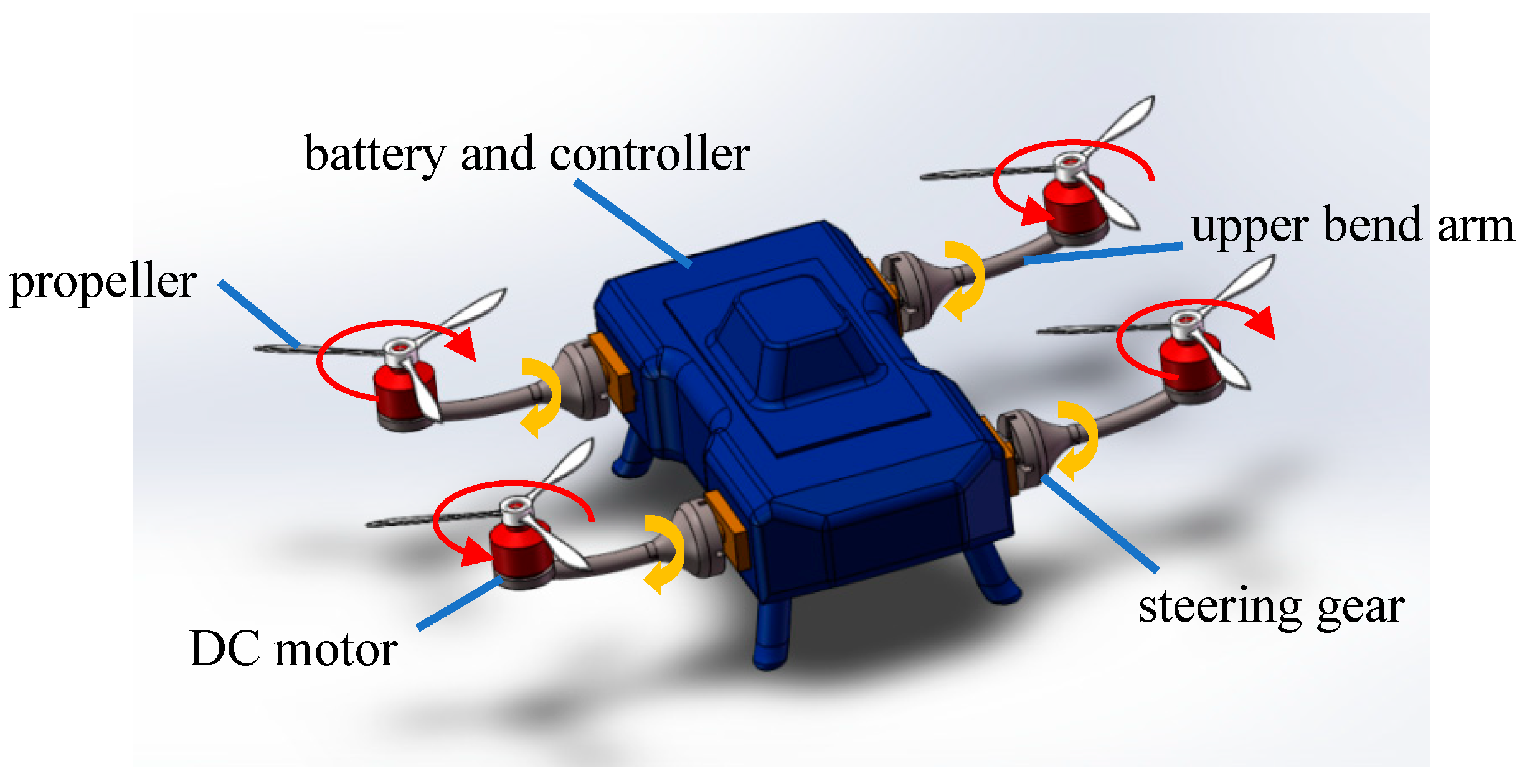
A four-rotor vehicle with adjustable arms is designed to be used in the switching operation of propulsion direction. The simple mechanism makes the vehicle more flexible and reliable. The use of only a single set of aerial rotors in both mediums greatly reduces cost, weight, and complexity compared to the other aerial underwater vehicle.

(2)

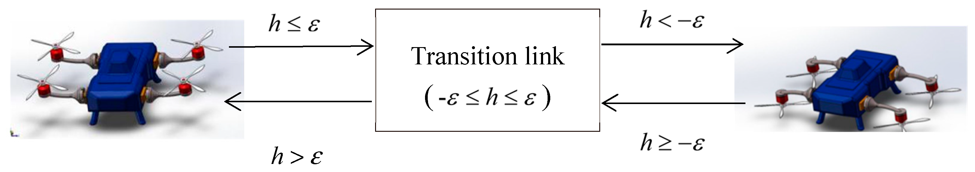
Mathematical models of the UAUV are deduced, the continuous dynamics are modeled by the Newton–Euler formalism, taking into account the effects of some additional variables, such as water resistance, buoyancy and their corresponding moments, normally neglected in aerial vehicles. Furthermore, a critical coefficient for air-to-water switching is presented to model the changed mass, force and moment in the cross-medium motion process.

(3)

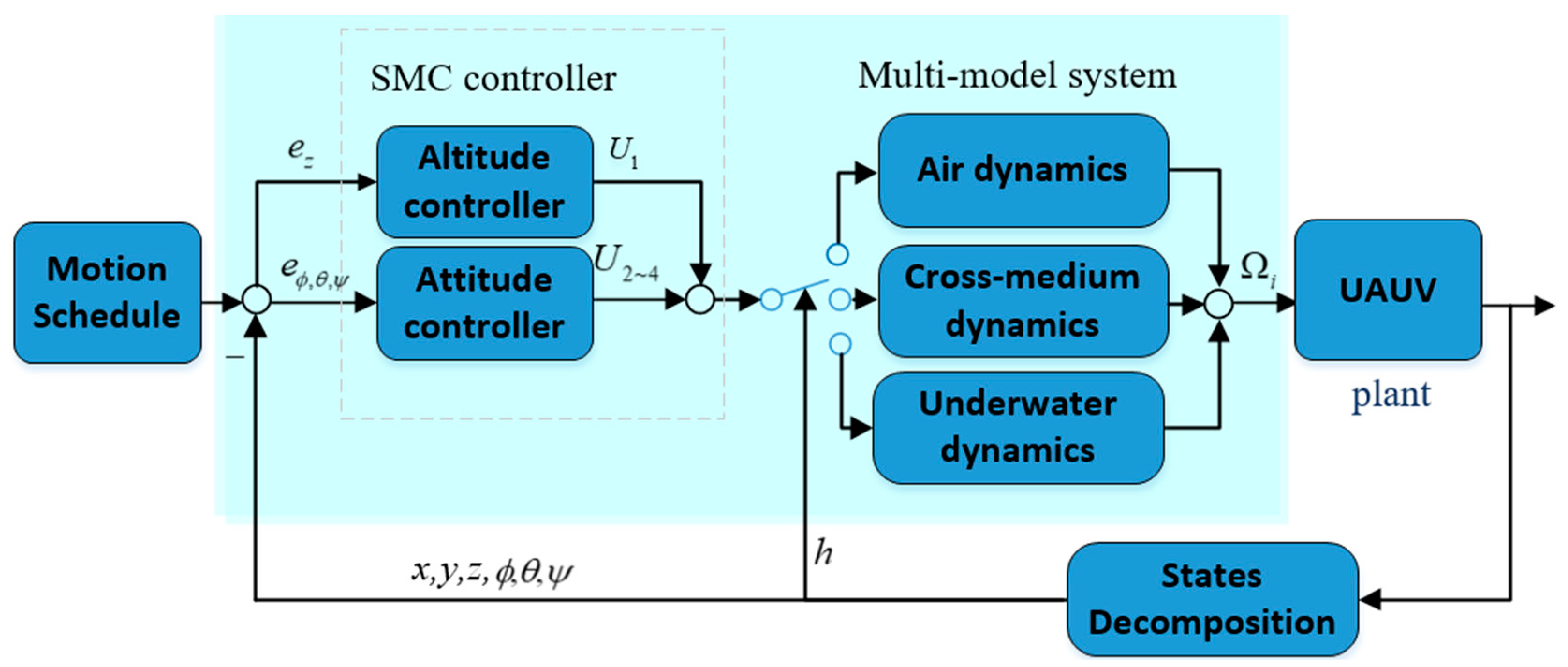
Robust sliding mode switching controllers are designed for effectively handling the cross-medium motion and achieving precise trajectory tracking. Finally, as a proof of concept, some simulation results for the trajectory tracking control are provided for the cross-medium unmanned vehicle.

The rest of this article is organized as follows. The second section introduces the reference frames and presents the modeling preliminaries of multi-rotor vehicles. The third section investigates the dynamics of cross-medium UAUVs according to the Newton–Euler laws. Section 4 designs a sliding mode control method and analyzes the switching control problems. Section 5 simulates the unmanned system and analyzes the attitude and position regulation of the vehicle. Finally, Section 6 gives a short conclusion and future work of the UAUVs.

2. Preliminaries

In this section, the mathematical model for the UAUV is illustrated. This model is basically obtained by representing the rotor-vehicle as a non-rigid body with adjustable rotor direction evolving in six dimensional space. Our aim is to provide the hybrid dynamic models of the cross-medium vehicle working in the air, air-to-water and underwater. Thus, the system dynamics can also be decomposed into three categories, detailed in Section 3. At the same time, the Newton–Euler equations are taken into account.

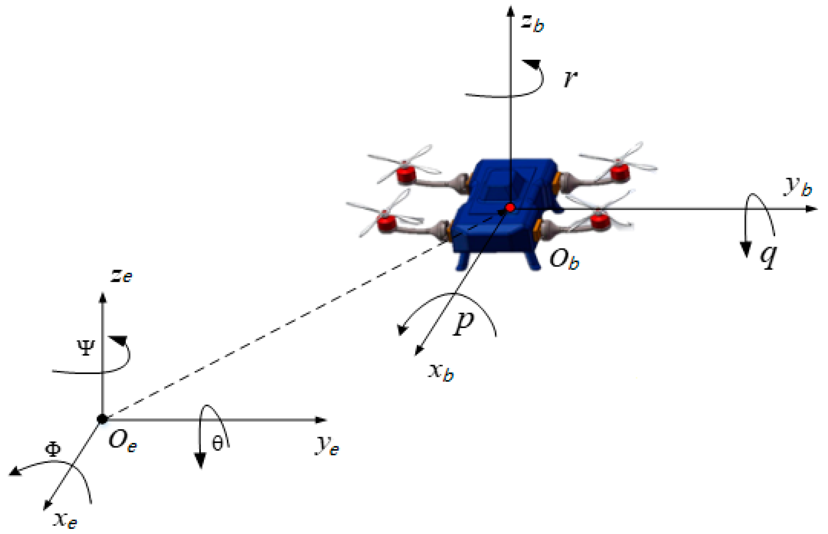
2.1. Reference Frames

This section first introduces the vehicle’s mechanical structure and its operation principle. Traditional hybrid vehicles have a multi-rotor structure, but the rotors are divided into two groups, which are used as power sources in the air and in the water respectively. Inspired by this model, a novel air-underwater configuration with only one set of rotors is proposed, shown in Figure 1.

The vehicle flies in the air like a four-rotor aircraft. However, in underwater navigation, the four rotors reverse 180 degrees through the steering gear, forming upward thrust to overcome the buoyancy of the vehicle underwater, and change the motion attitude of the vehicle by controlling the thrust of the four rotors, thus changing the trajectory of the vehicle underwater. It presents simple mechanical structure and mathematical model, good maneuverability and controllability and allows hovering.

In order to accurately describe the movement of the vehicle and establish a mathematical model of the vehicle, the body frame $O_b-x_b{y}_b{z}_b$ and the inertial frame $O_e-x_e{y}_e{z}_e$ are defined as shown in Figure 2. Note that $O_e$ is an East-North-Up (ENU) coordinate system and the axes of $x_e,y_e$ and $z_e$ point to the east, north and upper directions respectively. In order to express consistency for the vehicle motion, the definition of z-axis coordinates is upwards in both aerial and underwater cases in this paper. The position of the vehicle is written as $\xi ={\left[\begin{array}{ccc}x& y& z\end{array}\right]}^T$ and the attitude angle of the vehicle is denoted as $\eta ={\left[\begin{array}{ccc}\varphi & \theta & \psi \end{array}\right]}^T$ in the inertial frame $O_e$. In addition, the angle’s magnitude satisfies $\left|\eta \right|<{\eta }_L$ with the upper limit ${\eta }_L={\left[\begin{array}{ccc}\pi /2& \pi /2& 2\pi \end{array}\right]}^T$. This just means the vehicle can tilt the fuselage in motion, but the fuselage is not allowed to reverse. In the actual cases, the upper limits for the pitch and roll angles are usually less than $\pi /2$.

This paper describes the attitude of the aerial underwater vehicle using the Euler angle, and the rotation matrices $C_{\varphi }$, $C_{\theta }$ and $C_{\psi }$ in the angle $\varphi$, $\theta$ and $\psi$ are defined as:

$$C_{\varphi }=\left[\begin{array}{ccc}1& 0& 0\\ 0& c_{\varphi }& s_{\varphi }\\ 0& -s_{\varphi }& c_{\varphi }\end{array}\right],C_{\theta }=\left[\begin{array}{ccc}{c}_{\theta }& 0& -s_{\theta }\\ 0& 1& 0\\ s_{\theta }& 0& c_{\theta }\end{array}\right],C_{\psi }=\left[\begin{array}{ccc}{c}_{\psi }& s_{\psi }& 0\\ -s_{\psi }& c_{\psi }& 0\\ 0& 0& 1\end{array}\right]$$

where the element $s_{\varphi ,\theta ,\psi }$ are the sine function and $c_{\varphi ,\theta ,\psi }$ are the cosine function of the rotation angles. Obviously, the transformation from the inertial coordinate system to the body coordinate system can be obtained as:

$$R_{eb}=C_{\varphi }{C}_{\theta }{C}_{\psi }=\left[\begin{array}{ccc}{c}_{\theta }{c}_{\psi }& c_{\theta }{s}_{\psi }& -s_{\theta }\\ s_{\theta }{s}_{\varphi }{c}_{\psi }-c_{\varphi }{s}_{\psi }& s_{\theta }{s}_{\varphi }{s}_{\psi }+c_{\varphi }{c}_{\psi }& s_{\varphi }{c}_{\theta }\\ s_{\theta }{c}_{\varphi }{c}_{\psi }+s_{\varphi }{s}_{\psi }& s_{\theta }{c}_{\varphi }{s}_{\psi }-s_{\varphi }{c}_{\psi }& c_{\varphi }{c}_{\theta }\end{array}\right]$$

(1)

It can be seen that $R_{eb}$ is a direction cosine matrix expressed by the Euler angle of the unmanned vehicle.

2.2. Modeling of Multi-Rotor Vehicles

The mathematical models of four-rotor-driven vehicles are mostly described in the form of continuous differential equations. In general, it is assumed that the vehicle’s center of gravity coincides with the body-fixed frame origin and each propeller rotates at the angular velocity ${\Omega }_i$ (where the subscript i denotes the serial number of rotor, and $i=1,2,3,4$). Consequently, a force F_i is generated along or opposite to the z-direction relative to the body frame and a reaction torque M_i is produced on the vehicle body by each rotor expressed as:

$$\{\begin{array}{l}{F}_i=k_T{\Omega }_i^2\cdot \mathrm{sign}(h),\\ M_i={(-1)}^{i+1}{k}_Q{\Omega }_i^2.\end{array}\hspace{1em}\hspace{1em}i=1,2,3,4$$

(2)

where the two positive coefficients $k_T=c_T\rho r^4\pi$ and $k_Q=c_Q\rho r^5\pi$ denote the aerodynamic coefficient and the drag coefficient of the rotor respectively, and their magnitudes depend on the environmental medium density $\rho$, the radius of the propeller r, the thrust factor c_T and torque factor $c_Q$ of the designed rotors [26]. Furthermore, in the sign function, h denotes the vehicle altitude to the air–water interface.

The propellers represent the main source of thrust and can be designed specially in this hybrid configuration. Since the dynamic principle of the rotor structure is the same, aerial and aquatic propellers can present the same shape by optimizing the blade shape and size although the environments have different density. Therefore, the coefficients c_T, c_Q, the efficiency of engines and the energy delivered by the battery module have to be considered as the criteria to design the propeller shape (radius, width and curvature, et al.). Environmental density is directly proportional to the drag force and the added mass. Due to the large water density compared to the air density, it will generate high thrust forces with the same size and rotation speed to overcome the large movement resistance of the vehicles in the water. For convenience, the design process can be aided by the optimal propeller design software, such as OpenPro (OpenPro, Inc., Fountain valley, CA, USA), ShipPower (China state shipbuilding corporation limited, Shanghai, China).

The power system of the vehicle mainly includes rechargeable batteries, DC brushless motors and blades. Therefore, the magnitudes of the rotor’s angular velocities decide the system’s control inputs, which usually include the force and the torques created around a particular axis in body-fixed frame. In this section, the control signal can be defined as a vector $U={[\begin{array}{cccc}{U}_1& U_2& U_3& U_4\end{array}]}^T$, and the components U_1~4 denote the total thrust, the roll moment, the pitch moment and the yaw moment of the vehicle respectively. According to the dynamic principle of actuators, these control inputs can further be expressed by the following equation with the square vector of the rotor’s angular velocities as:

$$U=K{\left[\begin{array}{cccc}{\Omega }_1^2& {\Omega }_2^2& {\Omega }_3^2& {\Omega }_4^2\end{array}\right]}^T$$

(3)

where the coefficient K is a constant matrix for a symmetrical rigid multi-rotor vehicle. In addition, the arm’s length is denoted as $l$, then the coefficient matrix $K$ in (3) can be represented as the Kronecker product:

$$K=\left[\begin{array}{c}{k}_T\\ \sqrt{2}{k}_{T}l/2\\ \sqrt{2}{k}_{T}l/2\\ k_Q\end{array}\right]\otimes \left[\begin{array}{cccc}1& 1& 1& 1\\ 1& -1& -1& 1\\ 1& 1& -1& -1\\ 1& -1& 1& -1\end{array}\right]$$

(4)

Consequently, the dynamic model of the vehicle in frame O_b can be obtained by the Newton’s second law and theorem of moment of momentum as follows:

$$\begin{array}{l}{F}_b=m{\dot{v}}_b+m{\omega }_b\times v_b\\ M_b=J{\dot{\omega }}_b+{\omega }_b\times J{\omega }_b\end{array}$$

(5)

where m denotes the mass, F_b and M_b denote the resultant force and moment acting on the multi-rotor vehicle, and $v_b={\left[\begin{array}{ccc}u& v& w\end{array}\right]}^T$ denotes the linear velocity and ${\omega }_b={\left[\begin{array}{ccc}p& q& r\end{array}\right]}^T$ denotes the angular velocity. It is often convenient to let the origin of the frame O_b coincide with the center of gravity, then the simplest form of the equations of motion is obtained when the body axes coincide with the principal axes of inertia. This implies that $J=diag{\left[\begin{array}{ccc}{J}_x& J_y& J_z\end{array}\right]}^T$, and $J_x$, $J_y$, $J_z$ are the inertia moments around x-axis, y-axis and z-axis respectively in the frame O_b. If this is not the case, the body-fixed coordinates can be rotated about their axes to obtain a diagonal inertia tensor by simply performing a principal axis transformation [27]. Then we have:

$$\begin{array}{l}\dot{\xi }=R_{eb}{}^T{v}_b\\ {\omega }_b=\dot{\varphi }{I}_1+C_{\varphi }(\dot{\theta }{I}_2+C_{\theta }(\dot{\psi }{I}_3\left)\right)\end{array}$$

(6)

where $I_1={\left[\begin{array}{ccc}1& 0& 0\end{array}\right]}^T$, $I_2={\left[\begin{array}{ccc}0& 1& 0\end{array}\right]}^T$, $I_3={\left[\begin{array}{ccc}0& 0& 1\end{array}\right]}^T$. Substituting $C_{\varphi }$, $C_{\theta }$, $C_{\psi }$ into the Equation (6), it also can be rewritten as:

$$\begin{array}{l}\dot{\xi }=\left[\begin{array}{ccc}{c}_{\theta }{c}_{\psi }& s_{\varphi }{s}_{\theta }{c}_{\psi }-c_{\theta }{s}_{\psi }& c_{\varphi }{s}_{\theta }{c}_{\psi }+s_{\varphi }{s}_{\psi }\\ c_{\theta }{s}_{\psi }& s_{\varphi }{s}_{\theta }{s}_{\psi }+c_{\varphi }{c}_{\psi }& c_{\varphi }{s}_{\theta }{s}_{\psi }-s_{\varphi }{c}_{\psi }\\ -s_{\theta }& s_{\varphi }{c}_{\theta }& c_{\varphi }{c}_{\theta }\end{array}\right]v_b\\ \dot{\eta }=\left[\begin{array}{ccc}1& s_{\varphi }t{g}_{\theta }& c_{\varphi }t{g}_{\theta }\\ 0& c_{\varphi }& -s_{\varphi }\\ 0& s_{\varphi }/c_{\theta }& c_{\varphi }/c_{\theta }\end{array}\right]{\omega }_b\end{array}$$

After that, by deriving the above formula, the dynamics of the vehicle can be expressed as:

$$\ddot{\xi }=A_{\xi }(U_{\xi }+d_{\xi })+B_{\xi }$$

(7)

$$\ddot{\eta }=A_{\eta }(U_{\eta }+d_{\eta })$$

(8)

where $U_{\xi }=U_1$, $U_{\eta }={\left[\begin{array}{ccc}{U}_2& U_3& U_4\end{array}\right]}^T$ are the control inputs, $d_{\xi }={\left[\begin{array}{ccc}0& 0& d_z\end{array}\right]}^{\mathrm{T}}$ and $d_{\eta }={\left[\begin{array}{ccc}{d}_{\varphi }& d_{\theta }& d_{\psi }\end{array}\right]}^{\mathrm{T}}$ denote the external disturbances for the force and the moment respectively, and the coefficient matrices $A_{\xi },B_{\xi },A_{\eta }$ can be represented as:

$$A_{\xi }=\frac{1}{m}\left[\begin{array}{c}{s}_{\varphi }{s}_{\psi }+c_{\varphi }{s}_{\theta }{c}_{\psi }\\ -s_{\varphi }{c}_{\psi }+c_{\varphi }{s}_{\theta }{s}_{\psi }\\ c_{\theta }{c}_{\varphi }\end{array}\right],B_{\xi }={\left[\begin{array}{ccc}0& 0& -g\end{array}\right]}^T,A_{\eta }=\left[\begin{array}{ccc}{c}_{\theta }& c_{\theta }{s}_{\varphi }& -c_{\theta }{c}_{\varphi }\\ 0& c_{\theta }{c}_{\varphi }& -c_{\theta }{s}_{\varphi }\\ 0& s_{\varphi }& c_{\varphi }\end{array}\right]J$$

In practical applications, the values of the position $\xi$ and the attitude $\eta$ can be measured by the sensors, such as Global Positioning Sysrtem (GPS), altimeter, gyroscope.

3. Dynamics of Cross-Medium Unmanned Aerial Underwater Vehicles (UAUVs)

By contrast with the single-medium operation environment, the cross-medium environment complicates the modeling analysis and stable continuous control of the system. The density $\rho$ may jump aggressively from one value to another. In this case, the jump occurs when the vehicle’s altitude h reaches the air-water interface, i.e., $h:=0$. In order to distinguish different external environments of the vehicle, a critical layer thickness of water surface is defined as $\epsilon$, the value depends on the physical size of the vehicle and the model over-process requirements and $\epsilon \to 0$. The mode switching for the cross-medium behavior of an aerial underwater vehicle is shown in Figure 3.

Therefore, operational modes of the cross-medium vehicles can be divided into three categories according to the current altitude value h, which denotes a relative altitude between the vehicle and the air–water interface.

3.1. Dynamics when $h>\epsilon$

The aerial underwater vehicle is subjected to propeller thrust, air resistance, counter-torque generated by the propeller, and gyro moment generated by the attitude change during the movement. However, the air resistance and gyro moment can usually be ignored due to the small air density and small attitude change. Thus, only the propeller thrust, counter-torque and the gravity of the vehicle are considered during the vehicle’s motion in the air.

According to the reference frame definition in Section 2, the thrust generated by the propellers is $F_{\mathrm{m}}^b=\left[\begin{array}{ccc}0& 0& k_T{\displaystyle {\sum }_{i=1}^4{\Omega }_i^2}\end{array}\right]$ and the direction is upward, same to the $z_b$ axis. The motion equation of the vehicle in the inertial coordinate system can be derived as:

$$\left[\begin{array}{c}\ddot{x}\\ \ddot{y}\\ \ddot{z}\end{array}\right]=\left[\begin{array}{c}\frac{k_T(c_{\psi }{s}_{\theta }{c}_{\varphi }+s_{\psi }{s}_{\varphi }){\displaystyle {\sum }_{i=1}^4{\Omega }_i^2}}{m}\\ \frac{k_T(s_{\psi }{s}_{\theta }{c}_{\varphi }-c_{\psi }{s}_{\varphi }){\displaystyle {\sum }_{i=1}^4{\Omega }_i^2}}{m}\\ \frac{k_T{c}_{\theta }{c}_{\varphi }{\displaystyle {\sum }_{i=1}^4{\Omega }_i^2-mg}}{m}\end{array}\right]$$

(9)

The angular velocity of the vehicle in the inertial frame O_e:

$$\left[\begin{array}{c}\dot{\varphi }\\ \dot{\theta }\\ \dot{\psi }\end{array}\right]=\left[\begin{array}{c}p+p{s}_{\varphi }t{g}_{\theta }+r{c}_{\varphi }t{g}_{\theta }\\ q{c}_{\varphi }-r{s}_{\varphi }\\ q{s}_{\varphi }{\sec }_{\theta }+r{c}_{\varphi }{\sec }_{\theta }\end{array}\right]$$

(10)

Therefore, in the actual control, the motor’s speed output can be calculated. Finally, combined with the Formulas (3), (9) and (10), the motion model of the vehicle when $h>\epsilon$ satisfies:

$$\left[\begin{array}{c}\ddot{x}\\ \ddot{y}\\ \ddot{z}\\ \ddot{\varphi }\\ \ddot{\theta }\\ \ddot{\psi }\end{array}\right]=\left[\begin{array}{l}\frac{U_1}{m}(c_{\psi }{s}_{\theta }{c}_{\varphi }+s_{\psi }{s}_{\varphi })\\ \frac{U_1}{m}(s_{\psi }{s}_{\theta }{c}_{\varphi }-c_{\psi }{s}_{\varphi })\\ \frac{U_1}{m}{c}_{\theta }{c}_{\varphi }-g\\ \frac{\sqrt{2}l}{2}{U}_2-\dot{\theta }({\omega }_1-{\omega }_2+{\omega }_3-{\omega }_4)\\ \frac{\sqrt{2}l}{2}{U}_3+\dot{\varphi }({\omega }_1-{\omega }_2+{\omega }_3-{\omega }_4)\\ \frac{k_Q}{k_T}{U}_4\end{array}\right]$$

(11)

3.2. Dynamics when $h<-\epsilon$

The unmanned vehicle navigates in the water in a similar way to the air movement. The underwater vehicle is subjected to gravity, buoyancy, propeller thrust and resistance during movement. In addition, the moments subjected include heavy moments, floating moments, propeller thrust moments, resistance moments and gyro moments generated when the attitude changes.

Underwater vehicles are normally designed to satisfy the condition that the buoyancy force is slightly larger than the weight, which is important for safety reasons, and increasing weight or upward thrust is necessary for submersion. Therefore, in our configuration, the propeller arms of the vehicle will rotate by 180° after entering the water, so that the thrust of the propeller is reversed in an opposite direction to the z axis in the water, which is different from the convention used for some existing underwater vehicles.

In general, the motion of an underwater vehicle moving in six degrees of freedom (6DOF) at high speed will be highly nonlinear and coupled. However, in many underwater applications the vehicle will only be allowed to move at low speed, thus the Coriolis effects are smaller compared to the inertia effects of added mass, and the Coriolis effects of added mass are not considered in this paper. In addition, added mass can be seen as pressure-induced forces and moments due to a forced harmonic motion of the body which are proportional to the acceleration of the body. Since the movement of the vehicle in the water is also affected by the added mass, and the vehicle is approximately considered symmetrical, then the added mass along the three axes of the vehicle is only related to the acceleration and angular acceleration along the respective axes, and it can be expressed as:

$$m_k=m+diag\left[\begin{array}{cccccc}{m}_{\dot{u}}& m_{\dot{v}}& m_{\dot{w}}& m_{\dot{p}}& m_{\dot{q}}& m_{\dot{r}}\end{array}\right]$$

(12)

where $m_k$ represents the mass of the object in motion, $m_{\dot{u}},m_{\dot{v}},m_{\dot{w}}$ represent the added mass of axial motion in water, and $m_{\dot{p}},m_{\dot{q}},m_{\dot{r}}$ represent the added mass of rotating motion in water.

In the inertial frame O_e, the gravity of the vehicle in the water is in the opposite direction to the z-axis, but the buoyancy direction is the same as the z-axis. Furthermore, the matrix expression of the gravity and the buoyancy are converted to the body frame O_b as:

$$\left[\begin{array}{cc}{F}_{\mathrm{g}}^b& F_{\mathrm{b}}^b\end{array}\right]=R_{eb}=\left[\begin{array}{cc}0& 0\\ 0& 0\\ -m_{k}g& {\rho }_{w}gV\end{array}\right]=\left[\begin{array}{ll}{m}_{k}g{s}_{\theta }& -{\rho }_{w}gV{s}_{\theta }\\ -m_{k}g{s}_{\varphi }{c}_{\theta }& {\rho }_{w}gV{s}_{\varphi }{c}_{\theta }\\ -m_{k}g{c}_{\theta }{c}_{\varphi }& {\rho }_{w}gV{c}_{\theta }{c}_{\varphi }\end{array}\right]$$

(13)

where ${\rho }_{\mathrm{w}}$ is the density of water and V is the effective volume of the vehicle. Due to the high density of water, the resistance of the vehicle when moving in water cannot be ignored. In the frame O_b, the water flow resistance force $F_{rw}^b$ can be expressed as:

$$F_{rw}^b=0.5{\rho }_w{C}_{dw}S\left|v_b\right|v_b$$

(14)

where $C_{dw}$ is the dimensionless drag coefficient (for most underwater robots, $C_{dw}=0.8~1.0$), $\mathrm{S}=diag\left[\begin{array}{ccc}{\mathrm{S}}_x& S_y& S_z\end{array}\right]$ is the area in the direction of water flow velocity.

The thrust generated by the propellers is $F_{mw}^b=-F_m^b$, it’s direction is contrary to the $z_b$ axis. In summary, the external force $F_w^b$ of the UAUV can then be represented as:

$$\begin{array}{l}{F}_w^b=F_g^b+F_b^b+F_{rw}^b+F_{mw}^b\\ \hspace{1em}=\left[\begin{array}{c}(m_{k}g-{\rho }_{w}gV)s_{\theta }+0.5{\rho }_w{C}_{dw}{S}_x\left|u\right|u\\ -(m_{k}g-{\rho }_{w}gV)s_{\varphi }{c}_{\theta }+0.5{\rho }_w{C}_{dw}{S}_x\left|v\right|v\\ -(m_{k}g-{\rho }_{w}gV)c_{\theta }{c}_{\varphi }+0.5{\rho }_w{C}_{dw}{S}_x\left|w\right|w-k_T{\displaystyle {\sum }_{i=1}^4{\Omega }_i^2}\end{array}\right]\end{array}$$

(15)

The aerial underwater vehicle changes its attitude in the water by its torque. Since the origin of the body coordinate system is located at the center of gravity of the vehicle, the gravity does not generate the moment. The buoyancy center coordinates are assumed to be located on the $z_b$ axis in the frame O_b, and the buoyancy center coordinates are ${\left[x_f,y_f,z_f\right]}^T$ in the frame O_e. Then the buoyancy moment satisfies:

$$M_b^b=-F_b^b\left[\begin{array}{c}{z}_f{s}_{\varphi }{c}_{\theta }-y_f{c}_{\varphi }{c}_{\theta }\\ x_f{c}_{\varphi }{c}_{\theta }+z_f{s}_{\theta }\\ -y_f{s}_{\theta }-x_f{s}_{\varphi }{c}_{\theta }\end{array}\right]$$

(16)

where $F_b^b$ is the buoyancy of the vehicle underwater in the body coordinate system.

The thrust torque generated by the propeller in the water is similar to that in the air, but the thrust torque generated by the propeller in the water is opposite to that in the air due to the 180° rotation of the propeller, i.e., $M_{mw}^b=-M_m^b$ show in the 2~4th rows of the Formula (4). In addition, the change of the moving attitude in the underwater vehicle will produce the gyro moment as:

$$M_{gyrow}^b=-\left[\begin{array}{c}-J_{rw}q({\Omega }_1-{\Omega }_2+{\Omega }_3-{\Omega }_4)\\ J_{rw}p({\Omega }_1-{\Omega }_2+{\Omega }_3-{\Omega }_4)\\ 0\end{array}\right]$$

(17)

where $J_{rw}$ is the moment of inertia of the underwater motor and propeller.

If the aerial underwater vehicle changes its attitude in the water, it will also be affected by the resistance moment, which is proportional to the square of the angular velocity of the aerial underwater vehicle as $M_{rw}^b={\left[\begin{array}{ccc}{k}_x\left|p\right|p& k_y\left|q\right|q& k_z\left|r\right|r\end{array}\right]}^T$, where $k_x$, $k_y$ and $k_z$ are the resistance moment coefficients around the $x_b,y_b$ and $z_b$ axes in the body coordinate system. In summary, the external moment of the vehicle in the water can then be represented as:

$$\begin{array}{l}{M}_w^b=M_{mw}^b+M_b^b+M_{rw}^b+M_{gyrow}^b\\ =\left[\begin{array}{c}-\frac{\sqrt{2}}{2}{k}_{T}L({\Omega }_1^2-{\Omega }_2^2-{\Omega }_3^2+{\Omega }_4^2)-k_x\left|p\right|p-F_b^b(z_1{c}_{\theta }{s}_{\varphi }-y_1{c}_{\theta }{c}_{\varphi })+J_{rw}q({\Omega }_1-{\Omega }_2+{\Omega }_3-{\Omega }_4)\\ -\frac{\sqrt{2}}{2}{k}_{T}L({\Omega }_1^2+{\Omega }_2^2-{\Omega }_3^2-{\Omega }_4^2)-k_y\left|q\right|q-F_b^b(x_1{c}_{\theta }{c}_{\varphi }-z_1{s}_{\theta })+J_{rw}p({\Omega }_1-{\Omega }_2+{\Omega }_3-{\Omega }_4)\\ k_Q({\Omega }_1^2-{\Omega }_2^2+{\Omega }_3^2-{\Omega }_4^2)-k_z\left|r\right|r-F_b^b(-y_1{s}_{\theta }-x_1{c}_{\theta }{s}_{\varphi })\end{array}\right]\end{array}$$

(18)

If the aerial underwater vehicle fuselage is symmetrical about each coordinate system, the inertia matrix of its movement in the water can be set to $J_{\mathrm{w}}=diag\left[\begin{array}{ccc}{J}_{xxw}& J_{yyw}& J_{zzw}\end{array}\right]$. Similarly, the translational and rotational dynamics of the UAUV in water can be obtained by the Formulas (5), (15) and (18) as:

$$\left[\begin{array}{c}\dot{u}\\ \dot{v}\\ \dot{w}\\ \dot{p}\\ \dot{q}\\ \dot{r}\end{array}\right]=\left[\begin{array}{c}\frac{1}{m_k}\left[(m_{k}g-{\rho }_{w}gV)s_{\theta }+0.5{\rho }_w{C}_{dw}{S}_x\left|u\right|u\right]-wq+vr\\ \frac{1}{m_k}\left[-(m_{k}g-{\rho }_{w}gV)s_{\varphi }+0.5{\rho }_w{C}_{dw}{S}_y\left|v\right|v\right]-ur+wp\\ \frac{1}{m_k}\left[-(m_{k}g-{\rho }_{w}gV)c_{\theta }{s}_{\varphi }+0.5{\rho }_w{C}_{dw}{S}_z\left|w\right|w-k_T{\displaystyle {\sum }_{i=1}^4{\Omega }_i^2}\right]\\ \frac{1}{J_{xxw}}{\displaystyle \sum M_{xw}^b+\frac{J_{yyw}-J_{zzw}}{J_{xxw}}qr}\\ \frac{1}{J_{yyw}}{\displaystyle \sum M_{yw}^b+\frac{J_{zzw}-J_{xxw}}{J_{xxw}}rp}\\ \frac{1}{J_{zzw}}{\displaystyle \sum M_{zw}^b+\frac{J_{xxw}-J_{yyw}}{J_{zzw}}pq}\end{array}\right]$$

(19)

3.3. Dynamics when $-\epsilon \le h\le \epsilon$

For water and air cross-medium unmanned vehicles, the key processes include air-water transition (surface landing) and water-air transition (surface takeoff). How to achieve a stable and reliable conversion between the water and the air is significant. The unmanned vehicle can splash into water, this method has certain advantages in both the water entering time and the falling distance. It is a suitable way for the air–water transition of the amphibious cross-medium vehicle.

The unmanned vehicle is in the semi-submersible dynamic process when $-\epsilon \le h\le \epsilon$. This kind of vehicle resolves the problem of sailing across the different mediums. The additional variables, such as water resistance, buoyancy, resistance moment, buoyancy moment and gyro moment, cannot be neglected. They are modeled for the completely underwater vehicle in Section 3.2. However, the values of these variables are related to the vehicle altitude, which are not same to the underwater case.

In order to model the dynamics of the UAUV in the environmental transition stage, a critical coefficient of the additional variables is defined as:

$$k_s=\frac{1}{2}(1-h/\epsilon ),\hspace{1em}\hspace{1em}-\epsilon \le h\le \epsilon$$

(20)

Thus, the critical coefficient k is inverse proportional to the altitude h, and obviously its magnitude satisfies $k_s\in [0,1]$. If the vehicle decreases to below the air-water interface, then k_s increases and the additional variables’ function will augment gradually to the underwater case, and vice versa. Similarly, the dynamics can be deduced from the Formula (19) as:

$$\left[\begin{array}{c}\dot{u}\\ \dot{v}\\ \dot{w}\\ \dot{p}\\ \dot{q}\\ \dot{r}\end{array}\right]=\left[\begin{array}{c}\frac{1}{m_k}\left[(m_{k}g-{\rho }_{w}gV)s_{\theta }+0.5k_s{\rho }_w{C}_{dw}{S}_x\left|u\right|u\right]-wq+vr\\ \frac{1}{m_k}\left[-(m_{k}g-{\rho }_{w}gV)s_{\varphi }+0.5k_s{\rho }_w{C}_{dw}{S}_y\left|v\right|v\right]-ur+wp\\ \frac{1}{m_k}\left[-(m_{k}g-{\rho }_{w}gV)c_{\theta }{s}_{\varphi }+0.5k_s{\rho }_w{C}_{dw}{S}_z\left|w\right|w-k_T{\displaystyle {\sum }_{i=1}^4{\Omega }_i^2}\right]\\ \frac{1}{J_{xxw}}{\displaystyle \sum k_s{M}_{xw}^b+\frac{J_{yyw}-J_{zzw}}{J_{xxw}}qr}\\ \frac{1}{J_{yyw}}{\displaystyle \sum k_s{M}_{yw}^b+\frac{J_{zzw}-J_{xxw}}{J_{xxw}}rp}\\ \frac{1}{J_{zzw}}{\displaystyle \sum k_s{M}_{zw}^b+\frac{J_{xxw}-J_{yyw}}{J_{zzw}}pq}\end{array}\right]$$

(21)

4. Controller Design

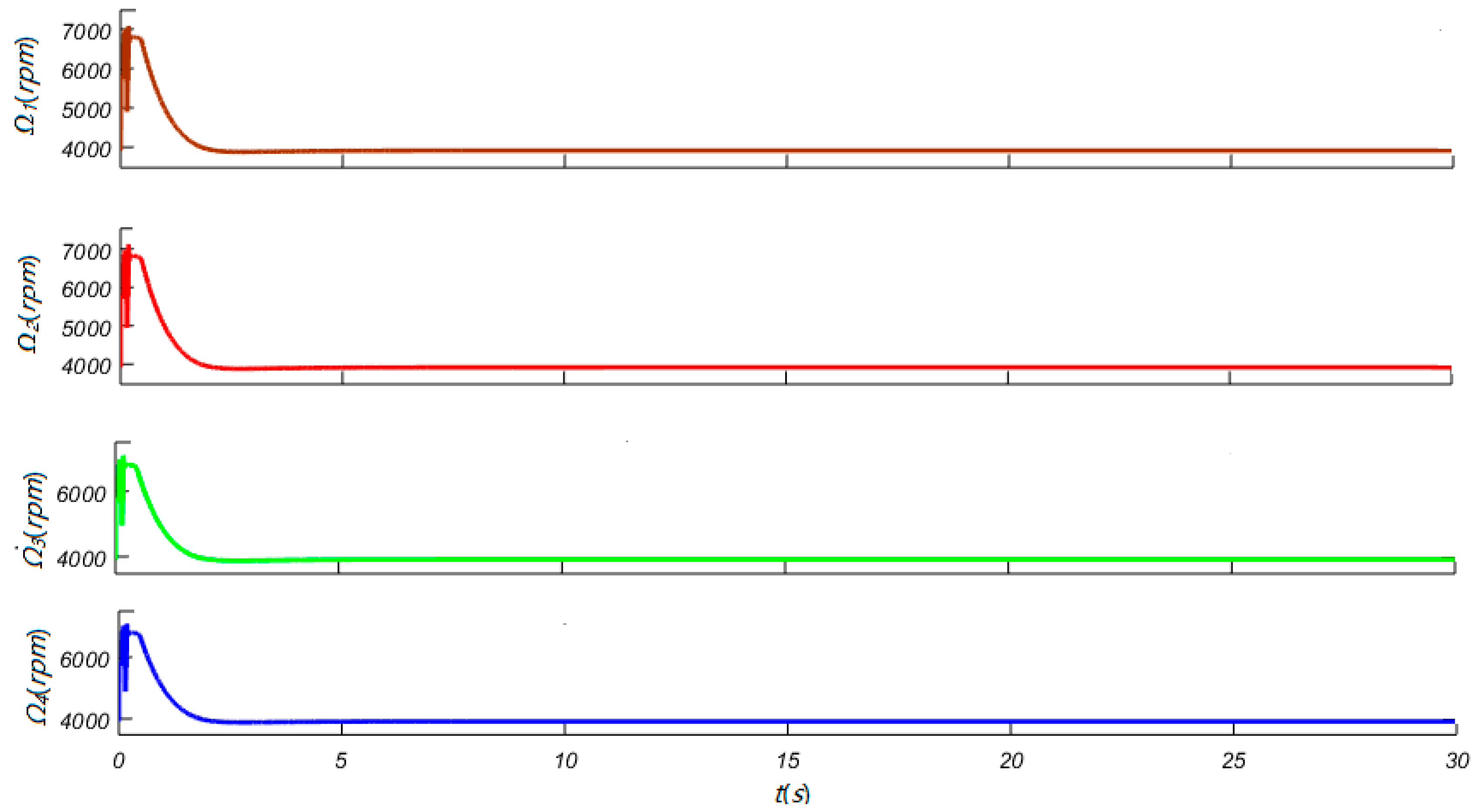
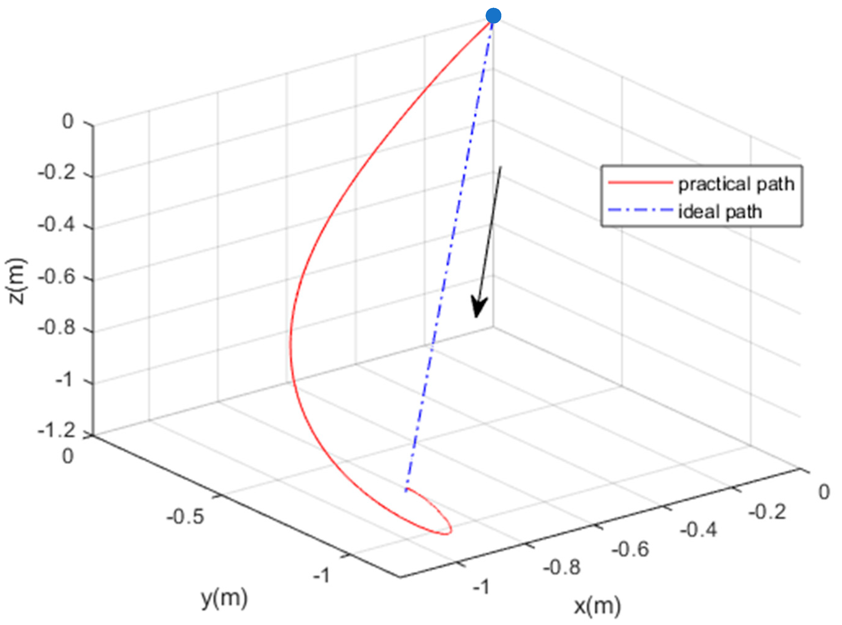
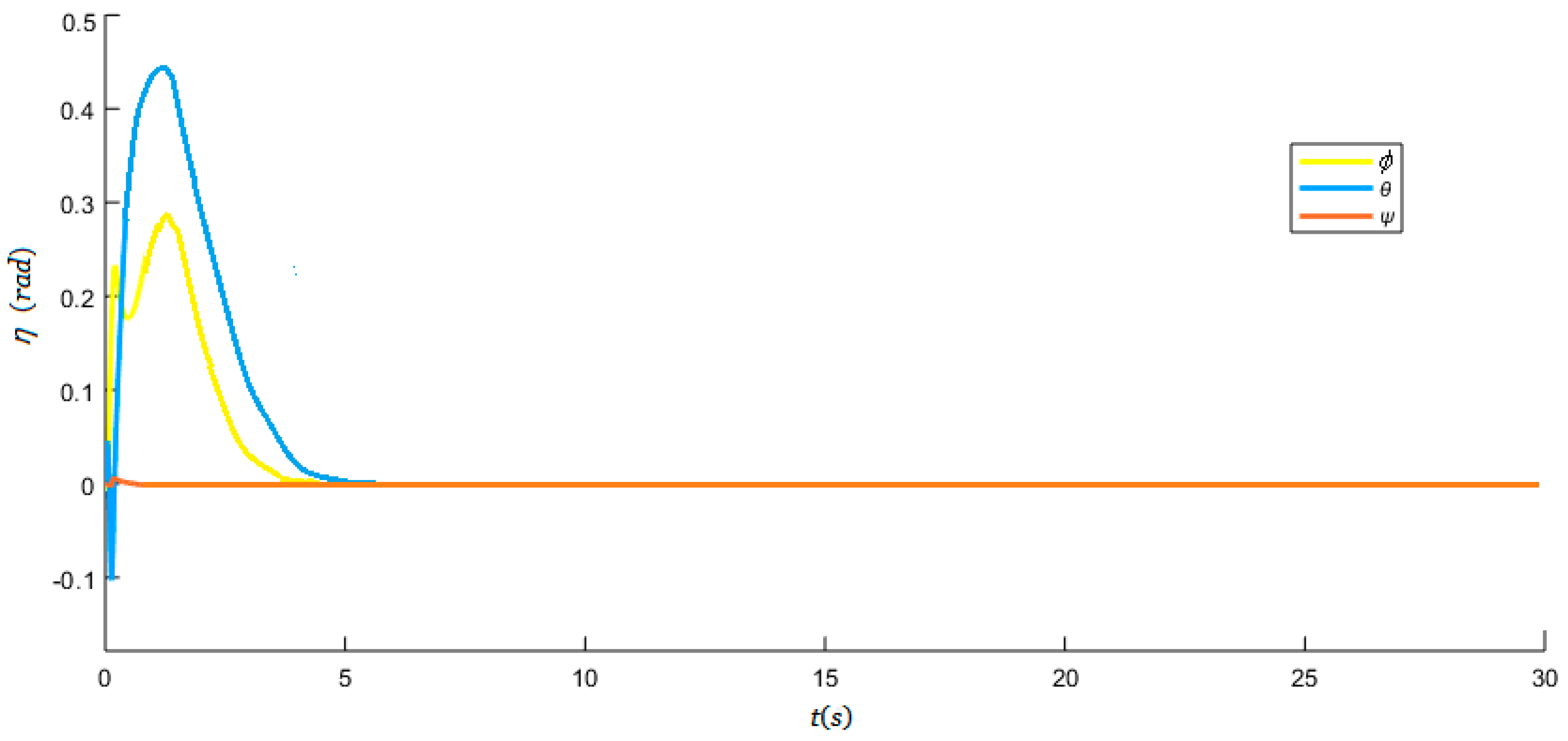
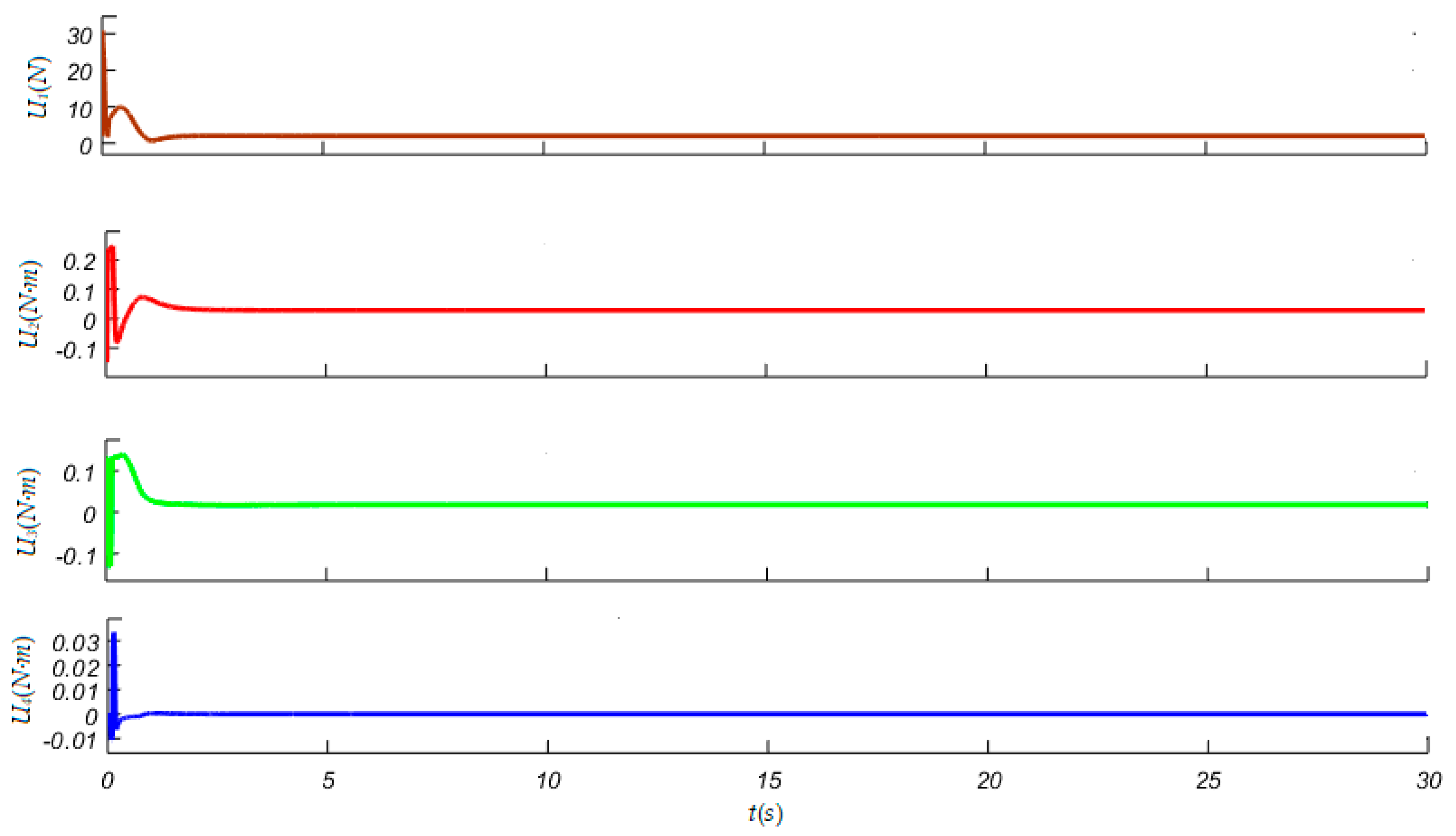
In this section, a non-linear control scheme is proposed, which provides the integrated control method of the air and underwater dynamics of the UAUV. The aerial underwater vehicle is a typical under-actuated system, and it faces a nonlinear and strong coupling environment. The advantages of sliding mode control are obvious, which is used to design the altitude controller and attitude controller of this unmanned system. Figure 3 shows the integrated control block diagram for the UAUV.

The deviations of altitude and attitude are the inputs of the SMC controller, and the controller outputs are the system inputs U_1~4. According to altitude h of the current vehicle distance from air-water interface, the dynamics of the multi-model system discussed in Section 3 is determined, and the angular velocities of the vehicle motor are calculated. Thus, a closed-loop nonlinear multi-model feedback control scheme is formed. The system outputs of the designed scheme mainly include the position and the attitude angles which can be measured directly.

In the above scheme depicted in Figure 4, the position loop is designed to attenuate the tracking position error which is expressed as ${\xi }_e={[\begin{array}{ccc}{x}_e& y_e& z_e\end{array}]}^T$. In addition, we substitute the position error ${\xi }_e$ into the Equation (7) and neglect the external disturbance temporarily, the following resultant error equation is deduced as:

$${\ddot{\xi }}_e=A_{\xi }{U}_1+B_{\xi }$$

(22)

Thus, the altitude sliding manifold of the vehicle can be defined as:

$${\sigma }_z=k_1^z{z}_e+k_2^z{\dot{z}}_e$$

(23)

where two coefficients $k_1^z$ and $k_2^z$ are constants. According to the SMC method, the system states are desired to remain on the manifold defined as ${\sigma }_z=0$, and the error dynamics can be written as $k_1^z{\dot{\xi }}_e+k_2^z{\ddot{\xi }}_e=0$. After that, we substitute the Equation (22) into this altitude second-order equation and get the equivalent control formula as:

$$U_1^{eq}=-(1/k_2^z)A_{\xi }{}^{-1}(k_1^z{\dot{z}}_e+k_2^z{B}_{\xi })$$

(24)

So long as the system dynamics are accurately modeled, $U_1^{eq}$ can maintain the altitude in the absence of external disturbances.

However, some unknown disturbances have to be considered in the real system, and the dynamics (22) can be represented as:

$${\ddot{\xi }}_e=A_{\xi }(U_1+d_{\xi })+B_{\xi }$$

(25)

where $d_{\xi }$ denotes the external disturbance mentioned before. To keep the system states still on the defined sliding mode manifold, a feedback control law of the system is redesigned as:

$$U_1=-(1/k_2^z)A_{\xi }{}^{-1}(k_1^z{\dot{z}}_e+k_2^z{B}_{\xi })-{\lambda }_z\cdot sat({\sigma }_z)$$

(26)

where ${\lambda }_z$ is a positive constant and $sat(\cdot )$ is a continuous saturation function defined as:

$$sat(x)=\{\begin{array}{cc}-1& x\le -\delta \\ x/\delta & \left|x\right|<\delta \\ 1& x\ge \delta \end{array},\hspace{1em}\hspace{1em}\delta >0.$$

(27)

where $\delta$ is the thickness of the boundary layer. For our sliding mode method, when the control error enters the given boundary layer, it will slip into the vicinity of zero in the boundary layer. Thus the saturation function is used to smooth out the control discontinuity around zero to reduce undesired chattering caused by imperfection switching of the discontinuous term. The performance of robustness is dependent on the thickness of the boundary layer, that means a thicker boundary layer may not be helpful to the robustness of the system.

In addition, the desired attitude can be calculated from the position errors, and the attitude error is obtained. After that, we consider the attitude loop used for attenuating the tracking attitude error ${\eta }_e={\left[\begin{array}{ccc}{\varphi }_e& {\theta }_e& {\psi }_e\end{array}\right]}^T$, Substituting the error ${\eta }_e$ into (8) and neglecting the environmental disturbance $d_{\eta }$, we get ${\ddot{\eta }}_e=A_{\eta }{U}_{\eta }$. Assume ${\lambda }_{\eta }$ is a positive constant, the corresponding control law obtained can be given by:

$$U_{\eta }=-(k_1^{\eta }/k_2^{\eta })A_{\eta }{}^{-1}{\dot{\eta }}_e-{\lambda }_{\eta }\cdot sat({\sigma }_{\eta })$$

(28)

where $k_1^{\eta }$, $k_2^{\eta }$ are constant control parameters.

5. Simulations

In this section, the dynamics and the proposed control method are verified on a simulation platform of an autonomous UAUV with 4 rotors. The numerical parameters used in the simulation are a mixture of previous, similar projects and measurements of the real platform. The mass of the simulation vehicle is 1.2 kg, and the length of its arm is 0.19 m, with a small body-volume of 10⁻³ m³, the maximum power of the motor is 202.8 W and the maximum rotational speed of the motor is 8500 rpm respectively. The detailed parameters used in the simulator are shown in Appendix A. In order to express clearly the work flow of the system, a flow diagram of the motion control process of the vehicle is presented in Figure 5.

At first we simulated the air position response and the underwater position response of the vehicle in the air and in the water single-medium environments in Section 5.1 and Section 5.2, respectively. Then, to verify the cross-medium characteristics of the unmanned vehicle, a cross-media control motion was performed in Section 5.3. Consequently, the vehicle navigation behavior is mainly divided into three cases: the air case, the underwater case and the transition case. In our platform, a critical layer thickness $\epsilon$ of the air–water interface is set to 0.25 m. Then for the case −0.25 < h < 0.25, the vehicle is in the transition mode. The air–water motion triggers the deceleration adjustment of the four rotors, and the rotors will reverse 180 degrees by the steering gears to change the thrust directions. Otherwise, the water–air motion triggers the acceleration adjustment of the four rotors and reverses the rotor directions similarly. In addition, for the case h > 0.25 and h < −0.25, the vehicle operates in the air mode and in the underwater mode respectively. Furthermore, the sliding mode controllers are used so as to control the vehicle’s position and attitude to infinitely close to the desired targets, and the desired attitude is calculated from the position errors of the vehicle, then the motor speeds are derived to drive the vehicle.

5.1. Air Position Response

In this case, we tested a straight-line flight control of the vehicle in the air. Set the original position O(0, 0, 0) of the vehicle on the water surface and the target position at the inertia coordinates T(5, 5, 5) in the air, and the route is a straight way from O to T. Consequently, the position response curve and attitude response curves can be obtained, shown in Figure 6 and Figure 7, respectively.

It can be seen that the aerial underwater vehicle can reach the specified position in a short time. Furthermore, this illustrates that although there is an overshoot of about 10% during its movement, the specified position can be reached within 5 s, and the actual path followed by the vehicle is very close to the desired straight-line path. In addition, the peak values of roll angle and pitch angle is 12.6° and 11.5° respectively, while the adjustment of yaw angle is relatively small.

The control inputs U_i (i = 1,2,3,4) of the vehicle are shown in the following Figure 8. In the initial acceleration stage, the upward thrust force U₁ increases rapidly to about 40 N, then falls back gradually and stabilized on 12 N which exactly counteracts its own gravity and maintained hovering state after vehicle reaches the target point. Furthermore, the moments U_2–4 of the three coordinate axes are also effective within the initial 5 s, which drive the vehicle to move to the target point by attitude adjustment during its ascending process. The outputs of the actuators for the system, i.e., the rotational speeds of the vehicle motors, are also shown in Figure 9.

It can be seen that the speeds of the motors increase rapidly to about 6800–7000 rpm, then decrease gradually to less than 4000 rpm and remain unchanged, which corresponds to the hovering state of the UAV. The speed differences of the four motors are not obvious because the upward thrust of the system is relatively large and the rotation moments are relatively small. When the UAV is in the vertical take-off and landing motion and hovering state, the four motors have the same speed.

5.2. Underwater Position Response

In this case, we tested a flight motion of the vehicle in the air. Set the original position O(0, 0, 0) of the vehicle on the water surface and the underwater target position at the inertia coordinates T(−1, −1, −1), and the route is a straight way from O to T. Consequently, the position response curve and attitude response curves can be obtained, as shown in Figure 10 and Figure 11, respectively. It can be seen that the aerial underwater vehicle can reach the set point steadily in the water. Because the water density is 1000 kg/m³, which is about 1000 times larger than the air density, it can produce high thrust with reduced motor speed. Furthermore, the peak values of roll angle and pitch angle are 16° and 24.2° respectively, while the adjustment of yaw angle is relatively small during the vehicle’s movement in water as shown in Figure 11.

The control inputs U_i (i = 1,2,3,4) of the vehicle are shown in the following Figure 12. In the initial acceleration stage, the upward thrust force U₁ increases rapidly to about 30 N, then falls back gradually and stabilizes on 3.5 N which is used to counteract the effects of its own gravity, buoyancy and water resistance. Furthermore, the moments U_2–4 of the three coordinate axes are also effective within the initial 5 s, which drive the vehicle to move to the target point by attitude adjustment during its descending process. The outputs of the actuators for the system, i.e., the rotational speeds of the vehicle motors are also shown in the Figure 13. It can be seen that the speeds of the motors increase rapidly to about 1410 rpm, then decrease gradually to less than 500 rpm and remained unchanged. However, the motor speeds are slower (one eighth) than those in the air.

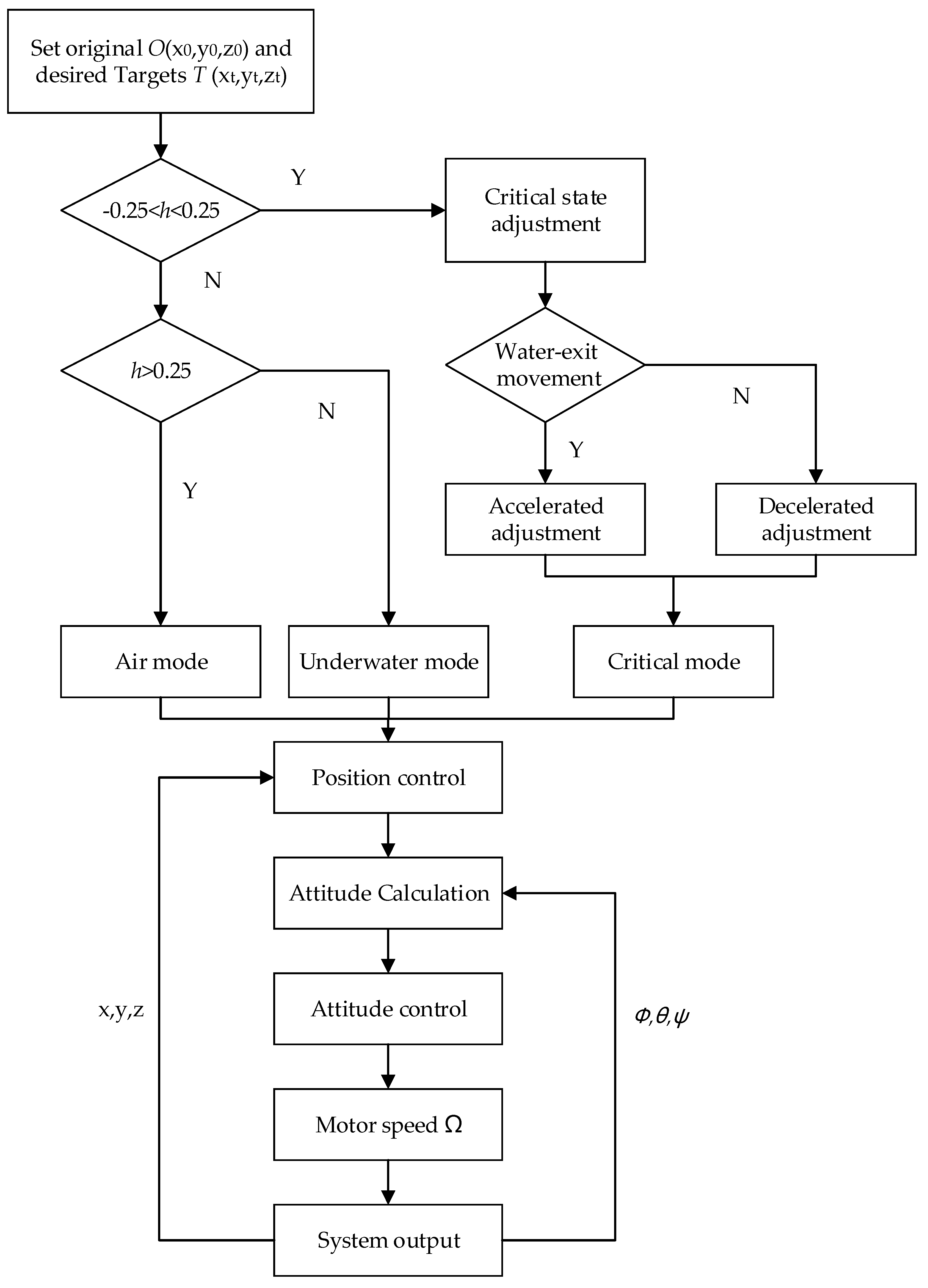
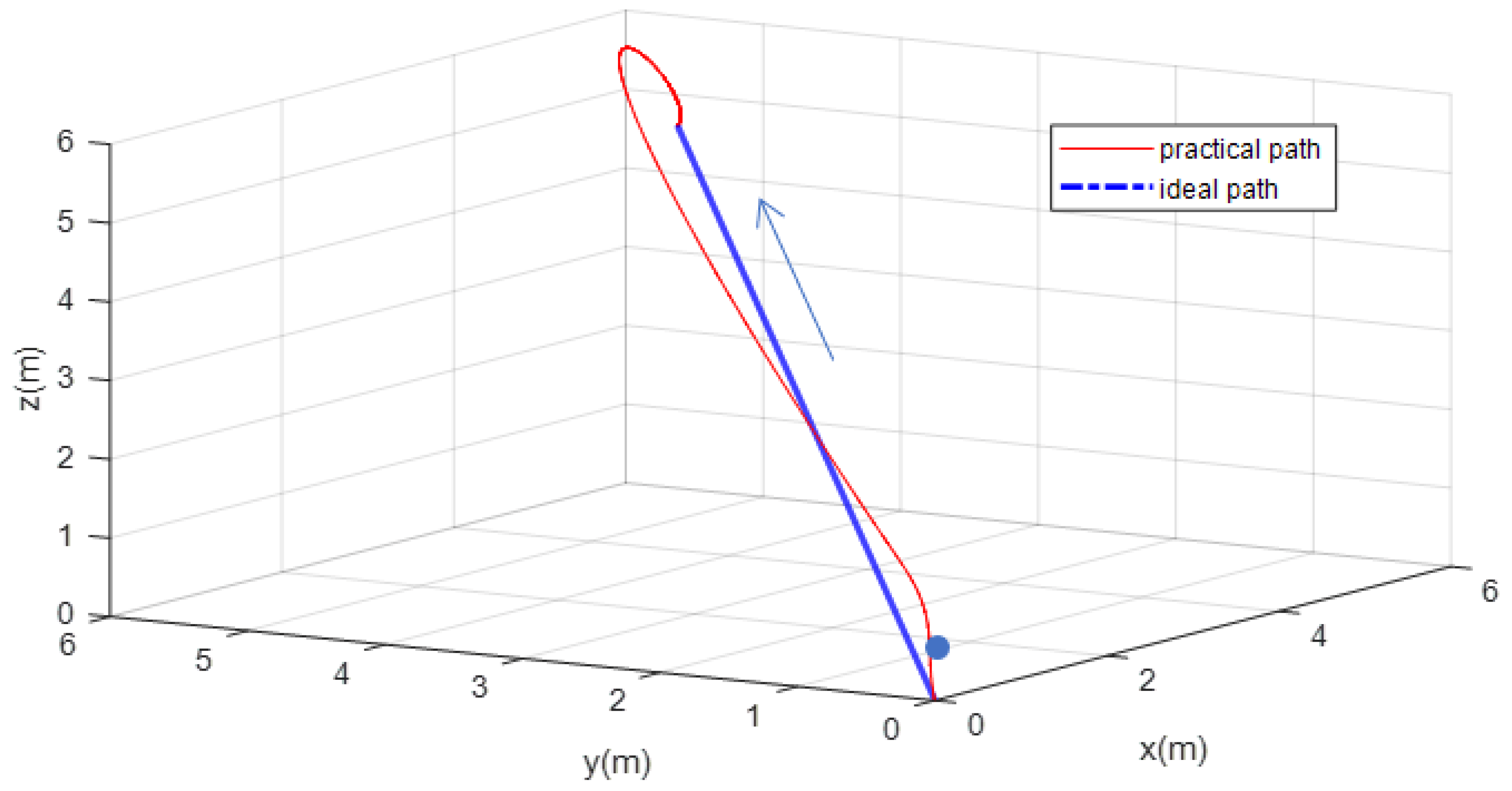
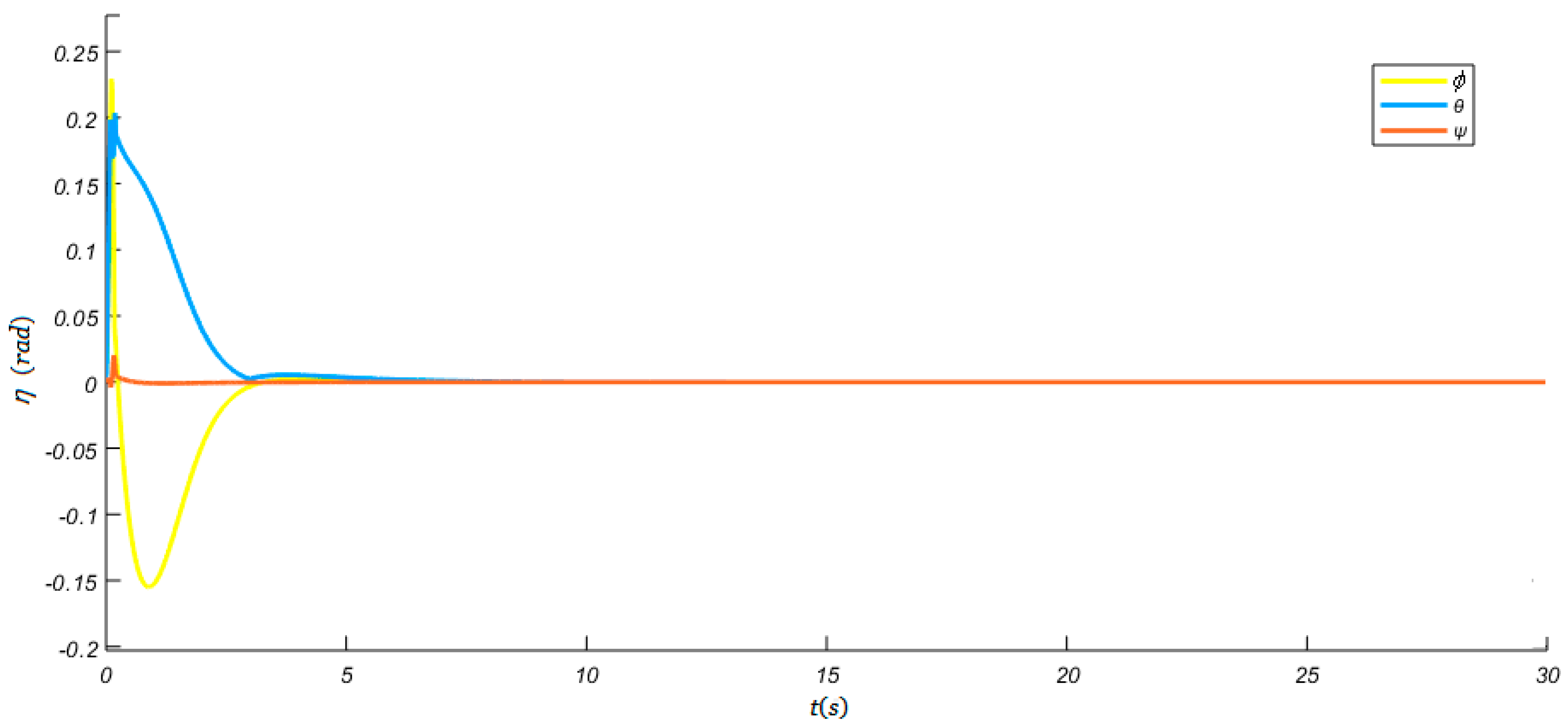
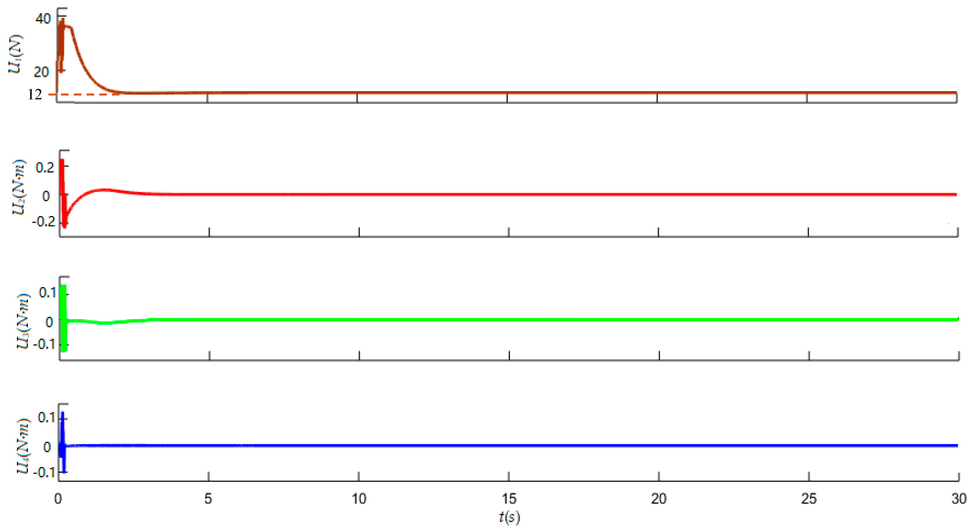
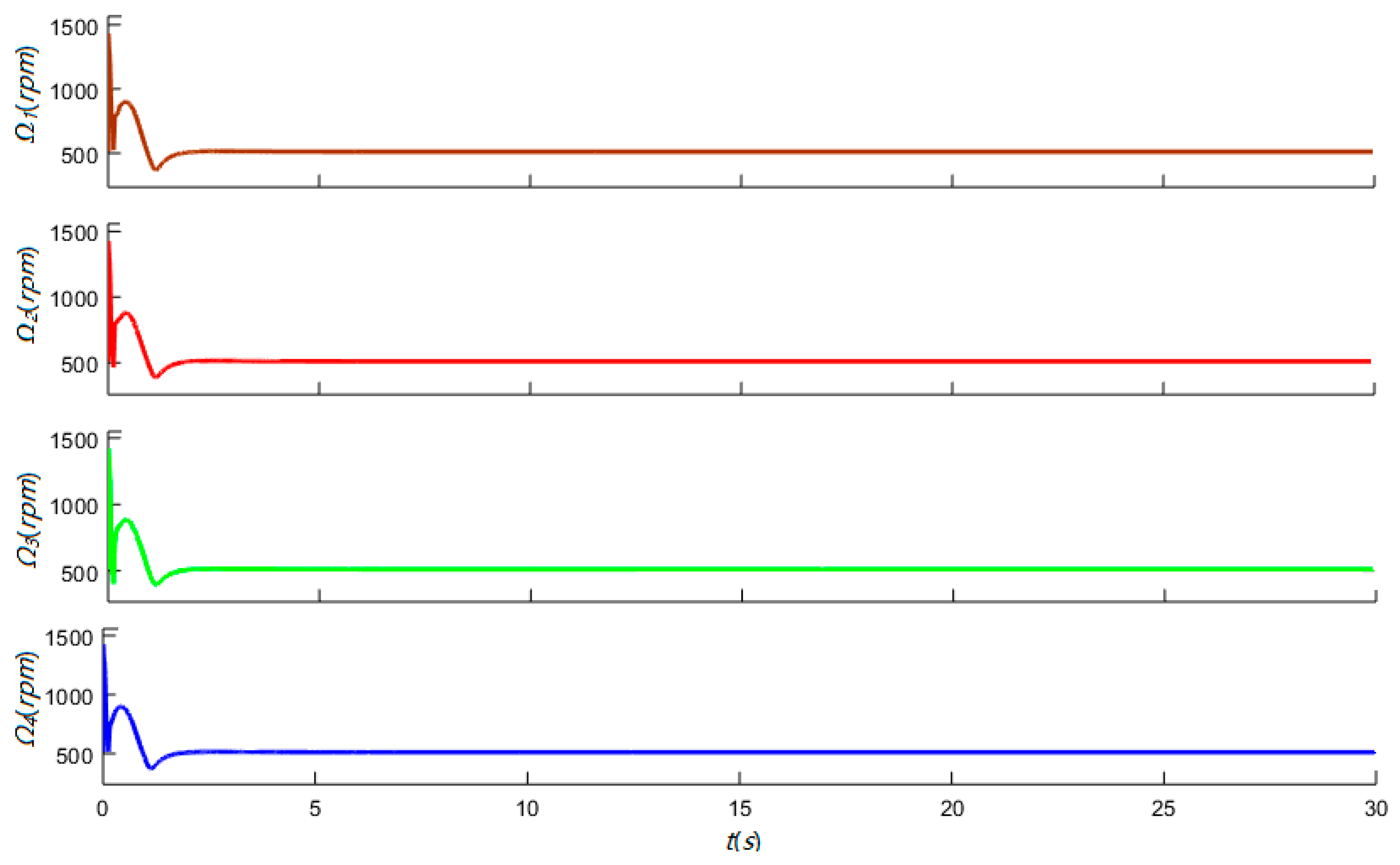
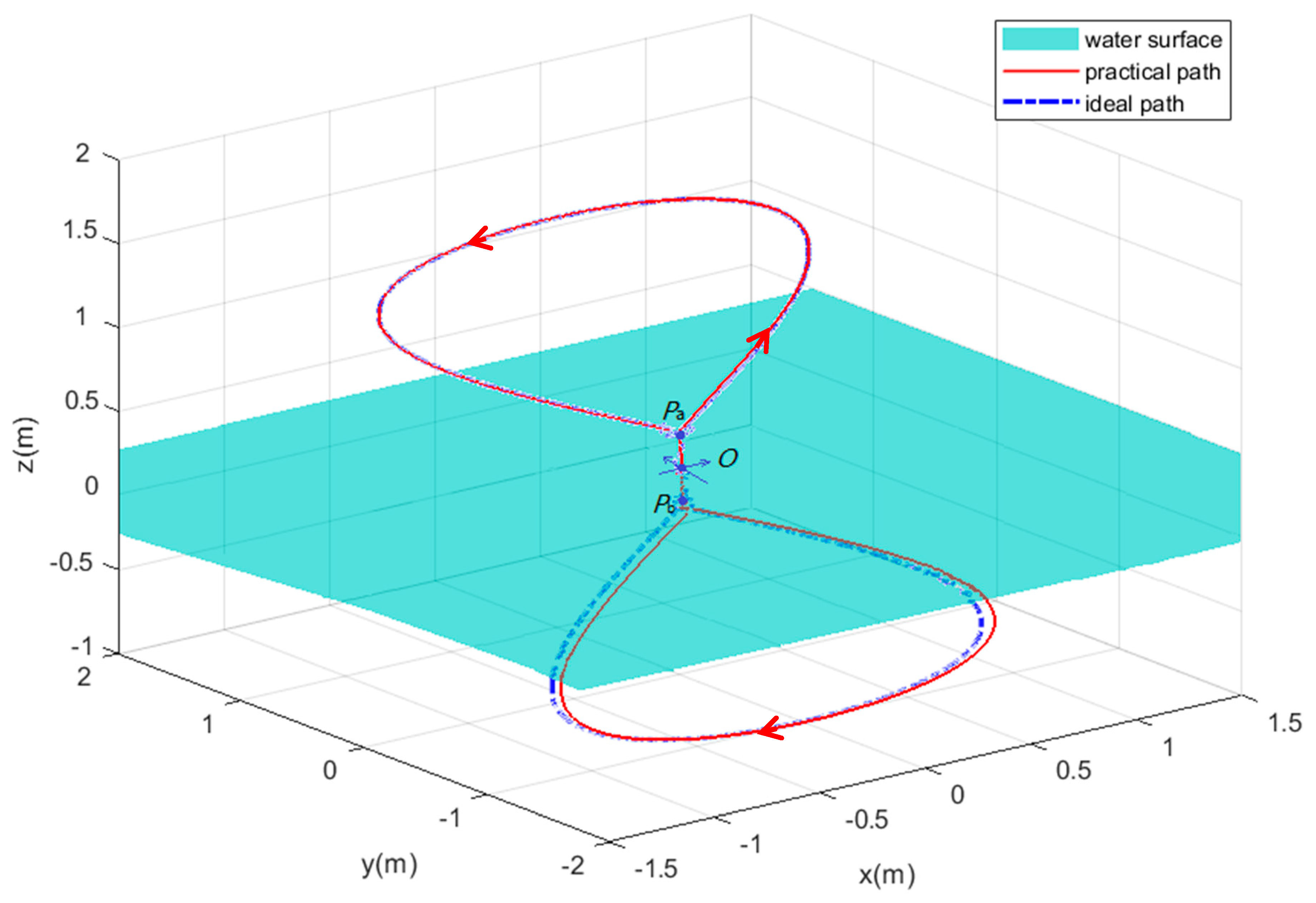
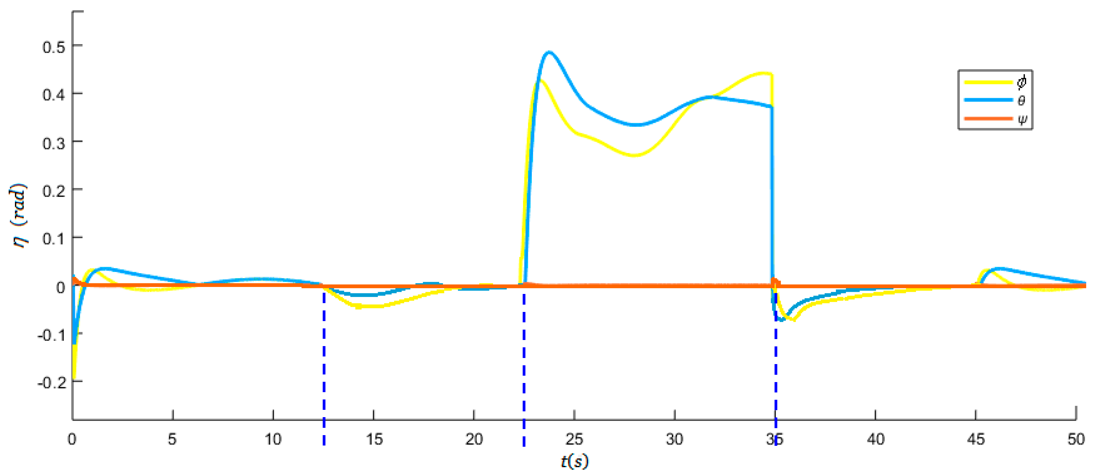
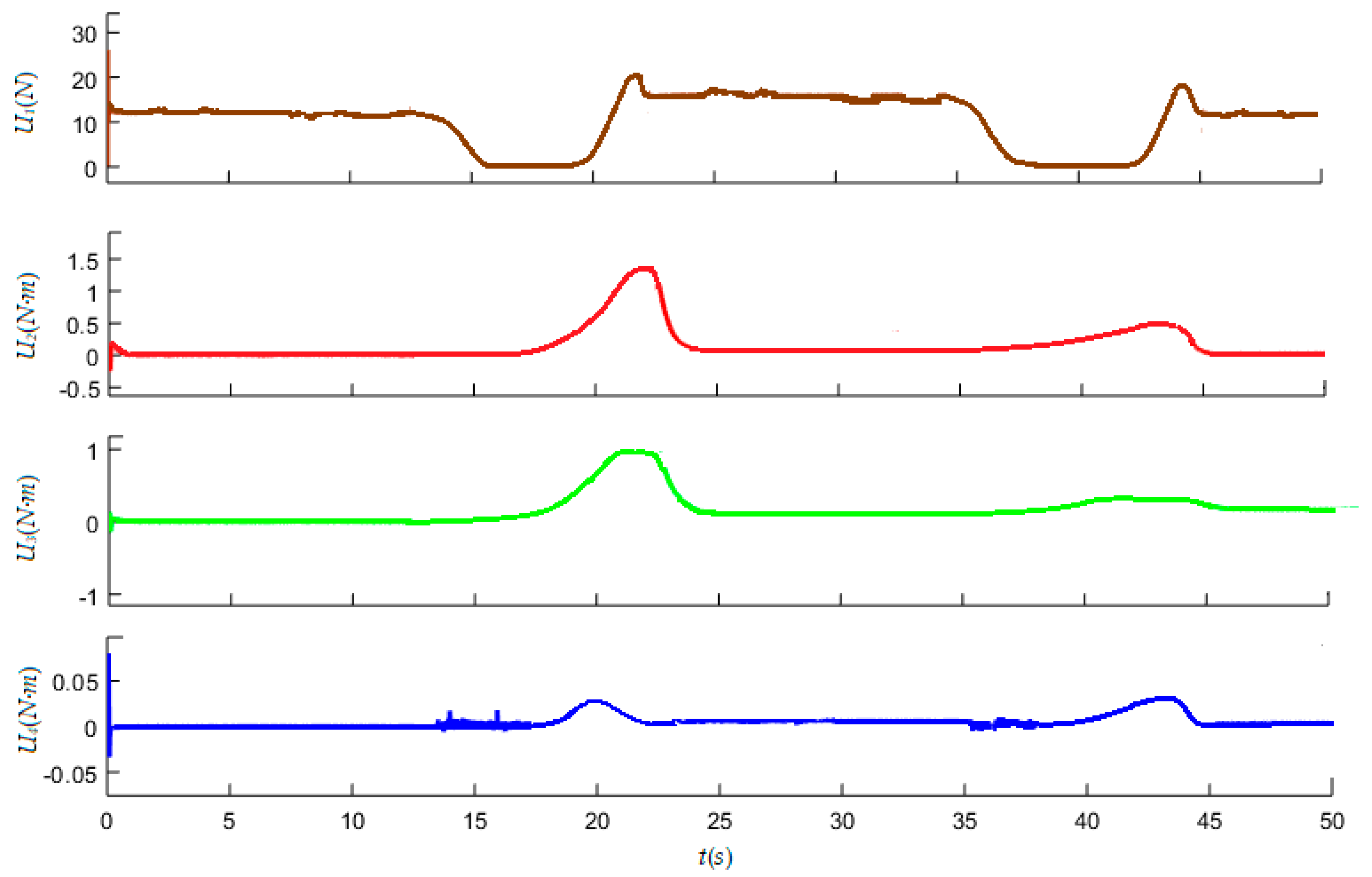
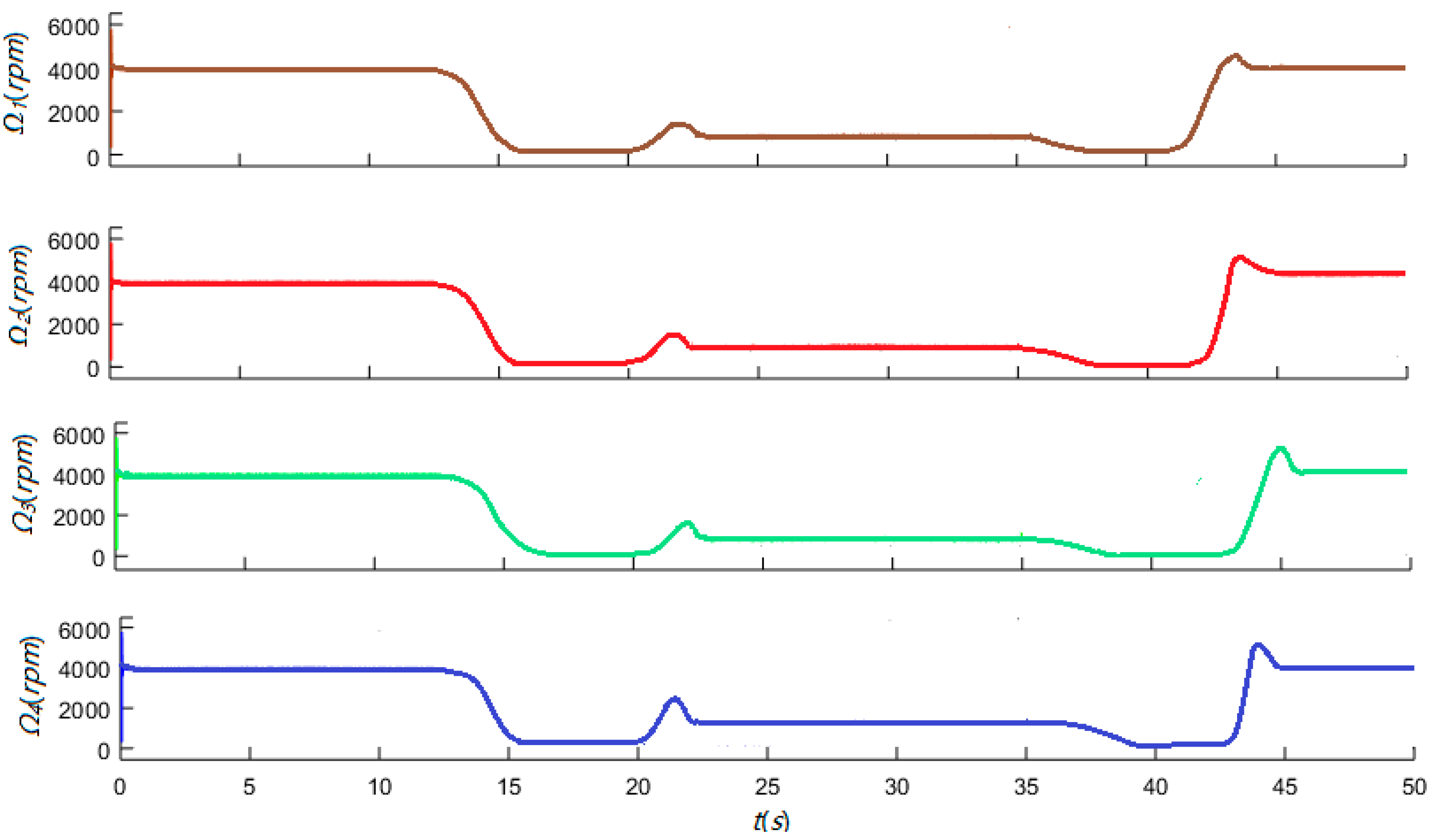
5.3. Aerial Underwater Vehicle Cross-Media Response

In this case, we test a cross-medium motion near the air-water interface, and we set the desired motion trajectory: $x_d=\sin (0.5t),y_d=\sin (0.25t),z_d=\sin (0.25t)+0.25\cdot sign(z)$ when the altitude of the vehicle satisfies $\left|z\right|\ge 0.25$. Otherwise, the aerial underwater vehicle is in vertical lift transition. As can be seen from the simulation result of the three-dimensional cross-medium trajectory shown in Figure 14, the vehicle first flies an arc in the air, then lands and enters the water from the point O, and dives through an arc trajectory, returning to the vicinity of the starting point. Moreover, point O is the incidence point on the water surface, and point P_a and point P_b are the vehicle state adjustment points respectively, and the vehicle moves vertically when its altitude is within the range $[-0.25,0.25]$. Therefore, the vehicle can travel across the medium and track the predetermined trajectory along the arrow directions.

In addition, Figure 15 shows that the attitude angles are adjusted to be small when $t\le 13\mathrm{s}$ at initial stage. However, the roll angle and pitch angle fluctuate slightly at t = 13 s and t = 35 s, which corresponded to the vehicle’s critical state adjustments of water-entering and water-exiting respectively. However, at t = 22.5 s, these two attitude angles suddenly increase to 0.4–0.5 rad and last for about 12.5 s, which corresponds to the vehicle’s motion in water.

The control inputs U_i (i = 1,2,3,4) of the vehicle are shown in the following Figure 16. In the initial stage, the upward thrust force U₁ is adjusted and stabilized on 12 N until t = 13 s. Then, the thrust force decreases to near zero and the vehicle’s arms are in the state of steering adjustment, and then the force gradually increases to about 16N at t = 20 s and lasts for a period of time. Thereafter, the reverse thrust force adjustment is made at t = 35 s, and the final effluent operation is completed. Furthermore, the moments U_2–4 of the three coordinate axes increase at about t = 20 s and the maximum is not more than 1 Nm, which drives the vehicle to adjust its attitude during the underwater motion. The rotational speeds of the vehicle motors are also shown in Figure 17. The motor speeds are approximately 4020 rpm and 560 rpm for the air condition and underwater condition respectively. In addition, all the rotational speeds of the motor have to undergo a process of first deceleration and then acceleration in the process of critical state adjustment.

6. Conclusions

This study evaluates the cross-medium motion of a quadrotor-like UAUV. The goal is to model the vehicle and simulate the autonomous control process both in the air and in the underwater environments. A hybrid vehicle configuration with only 4 rotors is proposed, and the thrust direction changes by the steering gears installed at the arm junctions. The simple mechanism makes the vehicle more flexible and reliable. The use of a single set of rotors in both mediums greatly reduces cost, weight, and complexity compared to other aerial underwater vehicle concepts. Without losing generality, the body frame and the inertial frame are defined to describe the position and attitude of the vehicle, and the transformation between these two frames is expressed as a direction cosine matrix of the vehicle’s Euler angles.

The thrust force and the reaction torque generated by each rotor are proportional to the square of the propeller’s angular velocities. Furthermore, the aerodynamic coefficient and the drag coefficient depend on the medium density, the radius of the propeller, the thrust and the torque coefficient. In our configuration, the aerial and aquatic propellers present the same shape, and the large water density generates high thrust forces with the same size and rotation speed to overcome the large movement resistance of the vehicles in the water. After that, the Quaternary control force and torque of the vehicle are defined. The system dynamics of the vehicle in the body frame are summarized and reconstructed as a second-order system based on Newton’s second law and the theorem of the moment of momentum.

For the cross-medium motion the of aerial underwater vehicle, a critical layer thickness of the water surface is first defined and the dynamics model switches according to the vehicle’s altitude h to the air–water interface. In our configuration, the thrust of the propeller is downward in the air to counteract the forces of gravity and acceleration, and is upward to submerge underwater. For the air environments, the air resistance and gyro moment are usually ignored to simplify the vehicle’s dynamics expression due to the small air density and small attitude change. However, the buoyancy, the resistance and the corresponding resistance moments and gyro moments generated when the attitude changes have to be considered in the dynamics due to the large water density. Besides, the added mass is considered and its magnitude is related to the acceleration and angular acceleration along the respective axes. Then the external force and moment are derived and represented. In particular, for the air–water and water–air transitions, a critical coefficient is presented to model the changed mass, force and moment in the cross-medium motion process. In addition, the sliding mode control method is used to design the altitude controller and attitude controller of this unmanned system, and a continuous saturation function is performed to reduce undesired chattering caused by imperfection switching of the method. Finally, the deduced dynamics and proposed control scheme are tested on the simulation platform of an autonomous UAUV in different scenarios.

In future work, it is important to apply our modeling and control method to the real cross-medium experimental platform, and study how to improve the vehicle’s maneuverability and stability, as well as investigating the influence of wind, wave, current and other disturbances on the system.

References

1. Hildreth, E. Capturing Images of a Game by An Unmanned Autonomous Vehicle. U.S. Patent 15/397,286, 4 April 2019. [Google Scholar]
2. Moud, H.I.; Shojae, A.; Flood, I. Current and Future Applications of Unmanned Surface, Underwater and Ground Vehicles in Construction. In Proceedings of the Construction Research Congress, New Orleans, LA, USA, 2–4 April 2018; pp. 106–115. [Google Scholar]
3. Kaub, L.; Seruge, C.; Chopra, S.D.; Glen, J.M.G.; Teodorescu, M. Developing an autonomous unmanned aerial system to estimate field terrain corrections for gravity measurements. Lead. Edge 2018, 37, 584–591. [Google Scholar] [CrossRef]
4. Zhong, Y.; Wang, X.; Xu, Y.; Wang, S.; Jia, T.; Hu, X.; Zhao, J.; Wei, L.; Zhang, L. Mini-UAV-Borne Hyperspectral Remote Sensing: From Observation and Processing to Applications. IEEE Geosci. Remote Sens. Mag. 2018, 6, 46–62. [Google Scholar] [CrossRef]
5. Soriano, T.; Pham, H.A.; Ngo, V.H. Analysis of coordination modes for multi-UUV based on Model Driven Architecture. In Proceedings of the 2018 12th France-Japan and 10th Europe-Asia Congress on Mechatronics, Tsu, Japan, 10–12 September 2018; IEEE: Piscataway, NJ, USA, 2018; pp. 189–194. [Google Scholar]
6. Morishima, S.; Hatano, M.; Sugeta, K.; Kozasa, T.; Momose, T.C.; Tani, T.; Ojika, H.; Matsuhashi, M.; Azuma, T. Design Method, Design Device, and Design Program for Cross-Sectional Shape of Fuselage. U.S. Patent 16/099,468, 21 March 2019. [Google Scholar]
7. Zhu, Z.; Guo, H.; Ma, J. Aerodynamic layout optimization design of a barrel-launched UAV wing considering control capability of multiple control surfaces. Aerosp. Sci. Technol. 2019, 93. [Google Scholar] [CrossRef]
8. Chen, Y.; Zhang, G.; Zhuang, Y.; Hu, H. Autonomous Flight Control for Multi-Rotor UAVs Flying at Low Altitude. IEEE Access 2019, 7, 42614–42625. [Google Scholar] [CrossRef]
9. Basri, M.A.M. Robust backstepping controller design with a fuzzy compensator for autonomous hovering quadrotor UAV. Iran. J. Sci. Technol. Trans. Electr. Eng. 2018, 42, 379–391. [Google Scholar] [CrossRef]
10. Owen, M.; Beard, R.W.; McLain, T.W. Implementing dubins airplane paths on fixed-wing uavs. In Handbook of Unmanned Aerial Vehicles; Springer: Dordrecht, The Netherlands, 2014; pp. 1677–1701. [Google Scholar] [CrossRef] [Green Version]
11. Nguyen, H.V.; Chesser, M.; Koh, L.P.; Rezatofighi, S.H.; Ranasinghe, D.C. TrackerBots: Autonomous unmanned aerial vehicle for real-time localization and tracking of multiple radio-tagged animals. J. Field Robot. 2019, 36, 617–635. [Google Scholar] [CrossRef] [Green Version]
12. Yuksek, B.; Vuruskan, A.; Ozdemir, U.; Yukselen, M.A.; Inlhan, G. Transition flight modeling of a fixed-wing VTOL UAV. J. Intell. Robot. Syst. 2016, 84, 83–105. [Google Scholar] [CrossRef]
13. Kamal, A.M.; Serrano, A.R. Design methodology for hybrid (VTOL+ Fixed Wing) unmanned aerial vehicles. Aeronaut. Aerosp. Open Access J. 2018, 2, 165–176. [Google Scholar] [CrossRef]
14. MahmoudZadeh, S.; Powers, D.M.W.; Zadeh, R.B. Introduction to autonomy and applications. In Autonomy and Unmanned Vehicles; Springer: Singapore, 2019; pp. 1–15. ISBN 978-981-13-2244-0. [Google Scholar]
15. He, Y.; Zhu, L.; Sun, G.; Dong, M. Study on formation control system for underwater spherical multi-robot. Microsyst. Technol. 2019, 25, 1455–1466. [Google Scholar] [CrossRef]
16. Bian, J.; Xiang, J. QUUV: A quadrotor-like unmanned underwater vehicle with thrusts configured as X shape. Appl. Ocean Res. 2018, 78, 201–211. [Google Scholar] [CrossRef]
17. Aminur, R.B.A.M.; Hemakumar, B.; Prasad, M.P.R. Robotic Fish Locomotion & Propulsion in Marine Environment: A Survey. In Proceedings of the 2018 2nd International Conference on Power, Energy and Environment: Towards Smart Technology (ICEPE), Haryana, India, 2 July 2018; IEEE: Piscataway, NJ, USA, 2018; pp. 1–6. [Google Scholar]
18. Kemp, M. Underwater Thruster Fault Detection and Isolation. In Proceedings of the AIAA Scitech 2019 Forum, San Diego, CA, USA, 7–11 January 2019; p. 1959. [Google Scholar] [CrossRef]
19. Jin, S.; Kim, J.; Kim, J.; Seo, T. Six-degree-of-freedom hovering control of an underwater robotic platform with four tilting thrusters via selective switching control. IEEE/ASME Trans. Mechatron. 2015, 20, 2370–2378. [Google Scholar] [CrossRef]
20. Alzu’bi, H.; Akinsanya, O.; Kaja, N.; Mansour, L.; Rawashdeh, O. Evaluation of an aerial quadcopter power-plant for underwater operation. In Proceedings of the 2015 10th International Symposium on Mechatronics and its Applications (ISMA), Sharjah, UAE, 8–10 December 2015; IEEE: Piscataway, NJ, USA, 2015; pp. 1–4. [Google Scholar] [CrossRef]
21. Maia, M.M.; Mercado, D.A.; Diez, F.J. Design and implementation of multirotor aerial-underwater vehicles with experimental results. In Proceedings of the 2017 IEEE/RSJ International Conference on Intelligent Robots and Systems (IROS), Vancouver, BC, Canada, 24–28 September 2017; IEEE: Piscataway, NJ, USA, 2017; pp. 961–966. [Google Scholar]
22. Mercado, D.; Maia, M.; Diez, F.J. Aerial-underwater systems, a new paradigm in unmanned vehicles. J. Intell. Robot. Syst. 2019, 95, 229–238. [Google Scholar] [CrossRef]
23. Neto, A.A.; Mozelli, L.A.; Drews, P.L.J.; Campos, M.F.M. Attitude control for an hybrid unmanned aerial underwater vehicle: A robust switched strategy with global stability. In Proceedings of the 2015 IEEE International Conference on Robotics and Automation (ICRA), Seattle, WA, USA, 26–30 May 2015; IEEE: Piscataway, NJ, USA, 2015; pp. 395–400. [Google Scholar]
24. Ravell, D.A.M.; Maia, M.M.; Diez, F.J. Modeling and control of unmanned aerial/underwater vehicles using hybrid control. Control Eng. Pract. 2018, 76, 112–122. [Google Scholar] [CrossRef]
25. Drews, P.L.J.; Neto, A.A.; Campos, M.F.M. Hybrid unmanned aerial underwater vehicle: Modeling and simulation. In Proceedings of the 2014 IEEE/RSJ International Conference on Intelligent Robots and Systems, Chicago, IL, USA, 14–18 September 2014; IEEE: Piscataway, NJ, USA, 2014; pp. 4637–4642. [Google Scholar]
26. Shi, D.; Dai, X.; Zhang, X.; Quan, Q. A practical performance evaluation method for electric multicopters. IEEE/ASME Trans. Mechatron. 2017, 3, 1337–1348. [Google Scholar] [CrossRef]
27. Fossen, T.I. Guidance and Control of Ocean Vehicles; Wiley: New York, NY, USA, 1996; pp. 28–29. [Google Scholar]
Figure 1. Configuration of the aerial underwater vehicle.
Jmse 07 00444 g001
Figure 2. Frames of the aerial underwater vehicle.
Jmse 07 00444 g002
Figure 3. Mode switching for the cross-medium behavior of aerial underwater vehicle.
Jmse 07 00444 g003
Figure 4. Aerial underwater vehicle control block diagram.
Jmse 07 00444 g004
Figure 5. Diagram of the motion control process of the unmanned aerial underwater vehicle (UAUV).
Jmse 07 00444 g005
Figure 6. Three-dimensional position graphic of the aerial underwater vehicle in the air.
Jmse 07 00444 g006
Figure 7. Attitude response curves of the aerial underwater vehicle in the air.
Jmse 07 00444 g007
Figure 8. Control inputs of the vehicle (Thrust force U1 and moments U2–4).
Jmse 07 00444 g008
Figure 9. Rotational speed outputs of the vehicle motors.
Jmse 07 00444 g009
Figure 10. Three-dimensional position graphic of the aerial underwater vehicle underwater.
Jmse 07 00444 g010
Figure 11. Attitude response curves of the vehicle underwater.
Jmse 07 00444 g011
Figure 12. Control inputs of the vehicle (Thrust force U1 and moments U2–4).
Jmse 07 00444 g012
Figure 13. Rotational speed outputs of the vehicle motors.
Jmse 07 00444 g013
Figure 14. Three-dimensional cross-medium trajectory of the UAUV.
Jmse 07 00444 g014
Figure 15. Cross-medium attitude response curves of the aerial underwater vehicle.
Jmse 07 00444 g015
Figure 16. Cross-medium control inputs of the vehicle (thrust force U1 and moments U2–4).
Jmse 07 00444 g016
Figure 17. Rotational speed outputs of the vehicle motors.
Jmse 07 00444 g017