Three-Dimensional Path Tracking Control of Autonomous Underwater Vehicle Based on Deep Reinforcement Learning

Abstract

In this paper, the three-dimensional (3D) path tracking control of an autonomous underwater vehicle (AUV) under the action of sea currents was researched. A novel reward function was proposed to improve learning ability and a disturbance observer was developed to observe the disturbance caused by currents. Based on existing models, the dynamic and kinematic models of the AUV were established. Deep Deterministic Policy Gradient, a deep reinforcement learning, was employed for designing the path tracking controller. Compared with the backstepping sliding mode controller, the controller proposed in this article showed excellent performance, at least in the particular study developed in this article. The improved reward function and the disturbance observer were also found to work well with improving path tracking performance.

1. Introduction

Autonomous underwater vehicle (AUV) path tracking control entails that AUV tracks the reference trajectory in a inertial coordinate system from a given initial state under the effective control strategy, and the global consistent and asymptotic stability of the position error should be ensured [1,2]. Underwater path tracking technology is the basis for autonomous underwater vehicles to accomplish complex tasks, and is widely used in all kinds of underwater works; for example, Dive, as a basic maneuver of the AUV, is usually performed by a three-dimensional (3D) spiral motion. The motion is a process of tracking for the cylindrical helix path. However, due to the underactuation, strong coupling, and nonlinear characteristics of the autonomous underwater vehicle and complex underwater environments, AUV three-dimensional path tracking has always been a very challenging field. Therefore, the research on the three-dimensional path tracking of AUV is significant [3].

Generally speaking, the methods used by underwater path tracking include: proportional integral derivative control method [4], backstepping control method [5], and sliding mode control method [6]. However, in recent years, artificial intelligence algorithms have been used in the control field of the autonomous underwater vehicle. Among them, reinforcement learning (RL), one of the machine learning methods, shows excellent results [7]. Because of the low requirements for the accurate system model and the ability to make judgments and autonomous optimization capability, reinforcement learning developed rapidly for AUV control.

Reinforcement learning (RL) has been widely used in robot control, traffic scheduling, communication control, and game decision making. In the field of path tracking control, reinforcement learning has many successful applications. El-Fakdi et al. proposed a high-level control system by using Reinforcement Learning Direct Policy Search methods to select actions for the AUV. The control policy was represented by a neural network whose input was a representation of the state and the output was probabilities of selected action. His method was easier to implement compared with other RL methods, but at the same time, simulated results showed a poor speed of convergence towards the minimal solution [8]. Carlucho et al. developed a deep RL framework based on the Actor-Critic theory, which took the available raw sensory information as input and output the continuous control actions as low-level control commands of AUV [9]. In another article [10], an expert agent-based system, based on a reinforcement learning agent, was proposed for self-adapting multiple low-level PID controllers in mobile robots. Fjerdingen compared and analyzed SARSA (State-Action-Reward-State-Action), CACLA (Continuous Actor Critic Learning Automaton), and supervised CACLA for continuous state and action spaces in his research about pipeline following for an AUV, and the skew normal distribution was used for exploration [7]. Chunyu et al. applied the Q-learning algorithm to learn the actuator action strategy directly in 3D path tracking, and a Cerebellar Model Arthrosis Controller (CMAC) neural network was applied to generalize the experience and accelerate the training [11]. In order to optimize the reference flight path, Pearre et al. [12] and Dunn et al. [13] took the flight path angle as the action of the reinforcement learning algorithm, constructed the reward function using energy consumption, time spent, and collision loss. In [14], a reinforcement learning approach for the airship model parameter identification was suggested by Ko et al., which reduced the control error caused by the model’s uncertainties. Shen and Dai suggested an adaptive iterative sliding mode control method based on reinforcement learning. The neural network was applied to optimize the control parameters, the chattering measurement variables and strengthen the learning signals were defined, and the online adjustment of the structure and parameters of the neural network was accomplished [15]. Wen-Yi combined a traditional feedback control method with supervised deep reinforcement learning, improving the performance of the system [16]. DDPG was first proposed by Lillicrapti in Proceedings of the International Conference on Learning Representations (ICLR) in 2016 [17]. It is based on Deterministic Policy Gradient (DPG) and incorporates the Actor-Critic theory while using the Deep Q-network (DQN) algorithm, which enabling DDPG algorithms to learn more effectively on continuous actions.

Most of the current deep reinforcement learning controllers output control signals from deep neural networks. However, some training processes of neural networks are simple and single, and some actual implementation limits and many real-world factors often fail to be considered [18]. For example, if the rudders angle is chosen to be the control output, the controller often adopts a more aggressive control signal to ensure the control effect. The change rate is high and the range of change is large. This obviously cannot apply to practical applications, and control outputs may even exceed the actual steering capability.

Ocean currents are ubiquitous; in the actual path tracking, the path tracking performance is always affected by currents. However, there are difficulties for deep neural networks to understanding the currents disturbance and make corresponding adjustments. In the process of reinforcement learning, the neural network constantly optimizes its own parameters through training. However, the reward value stay high continuously in the later stage of training, and the response of different states on the reward value is not obvious. That may cause negative influence to learning efficiency of the neural network, and more likely stagnates the learning.

In order to solve the AUV three-dimensional path tracking problem under the action of sea currents, AUV dynamic and kinematics model were proposed in this article, and the path tracking controller was designed basing on Deep Deterministic Policy Gradient (DDPG) algorithm. After that, the stable path tracking of cylindrical helix path was successfully carried out.

The work has been done in this article are:

(1)

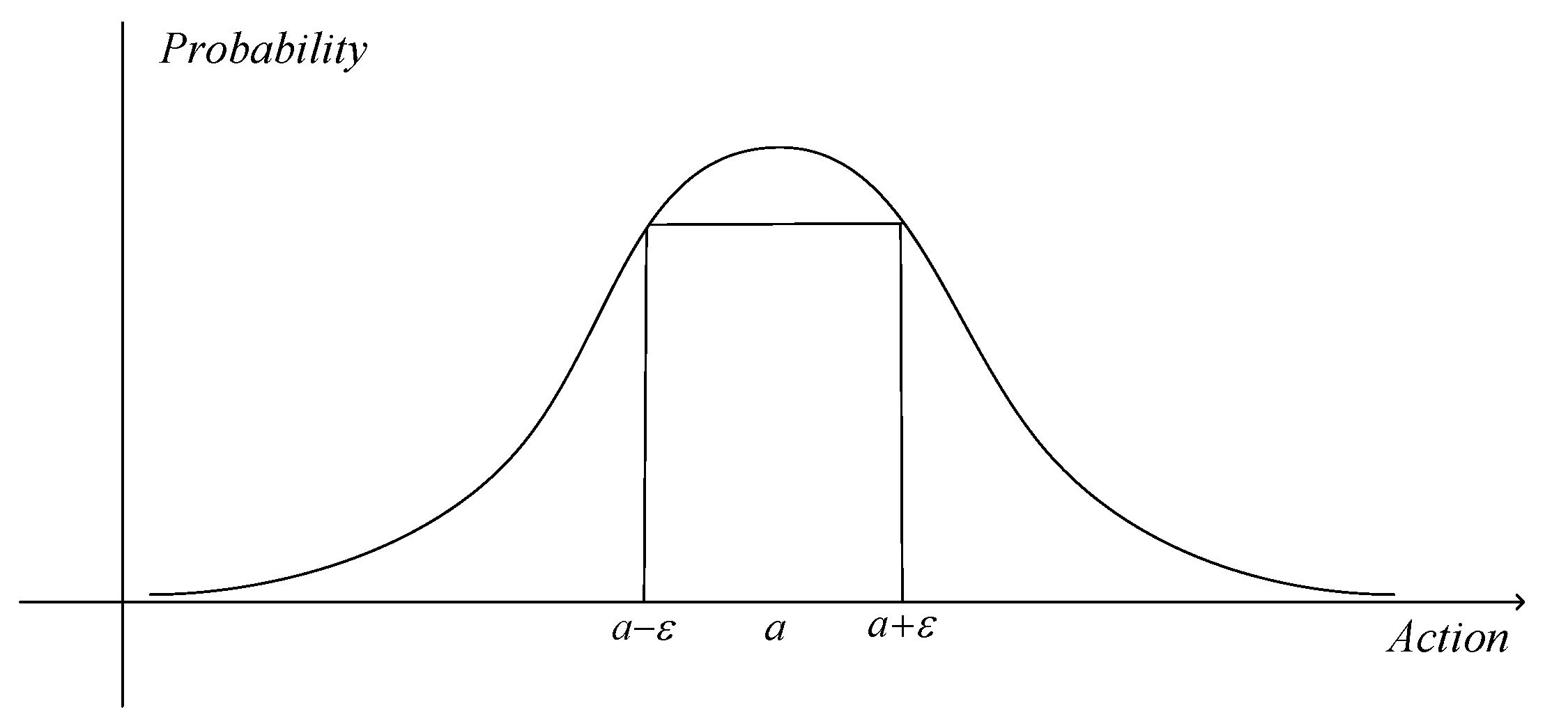
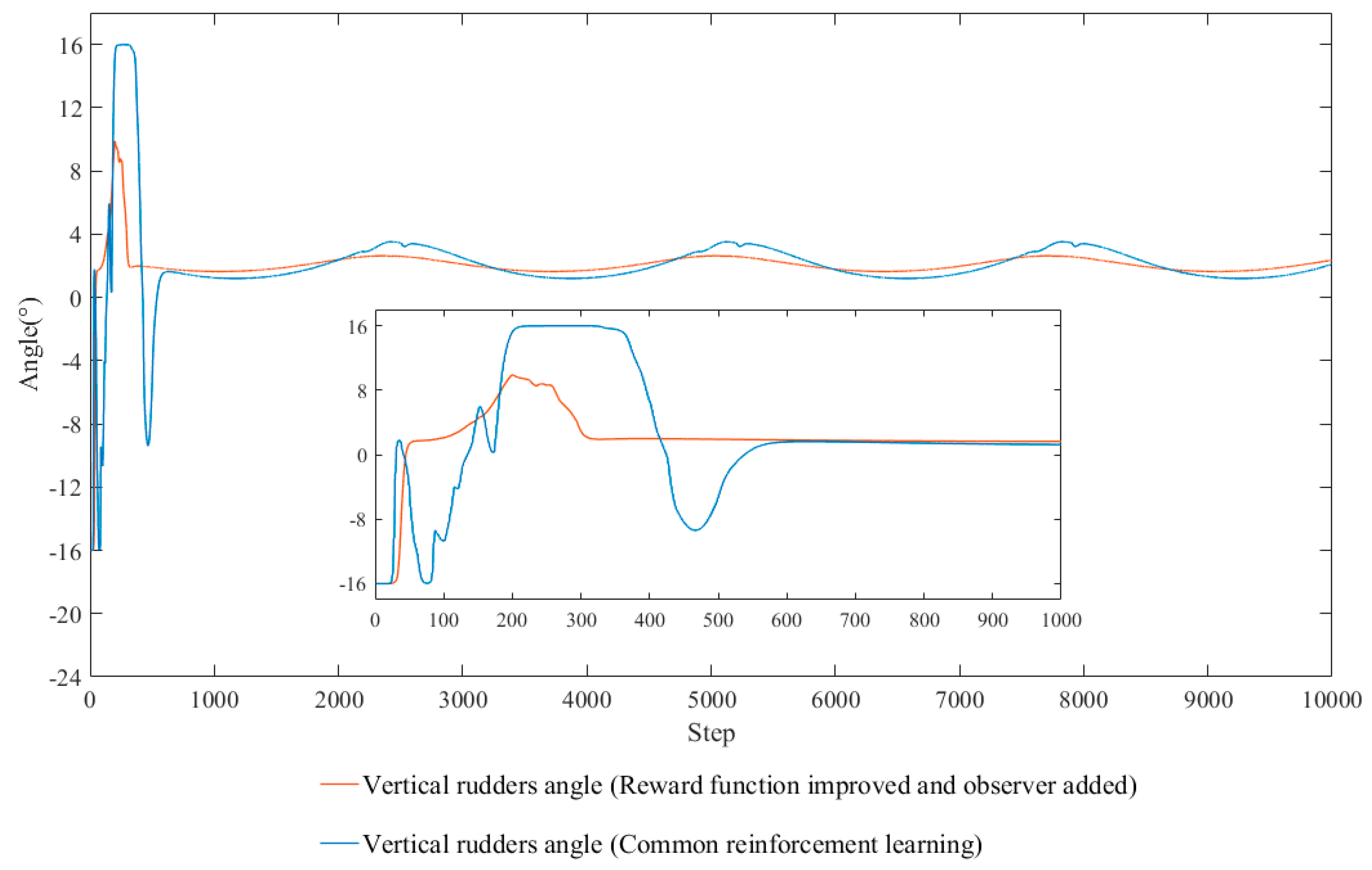
Rational optimization methods for reward function are studied. The rudders angle and their rate of change are used to form a second-order Gaussian function, which is a part of reward function. The steering frequency is successfully reduced, as the tracking performance was not affected.

(2)

As for the ocean currents disturbance, a current disturbance observer is added to perceive currents and optimize the output. The observer provides the capacity of anti-current and improves the tracking performance.

(3)

A boundary reward function is proposed to provide additional rewards when the AUV arrives at specific positions and maintains a correct angle, which improves the stability of path tracking.

(4)

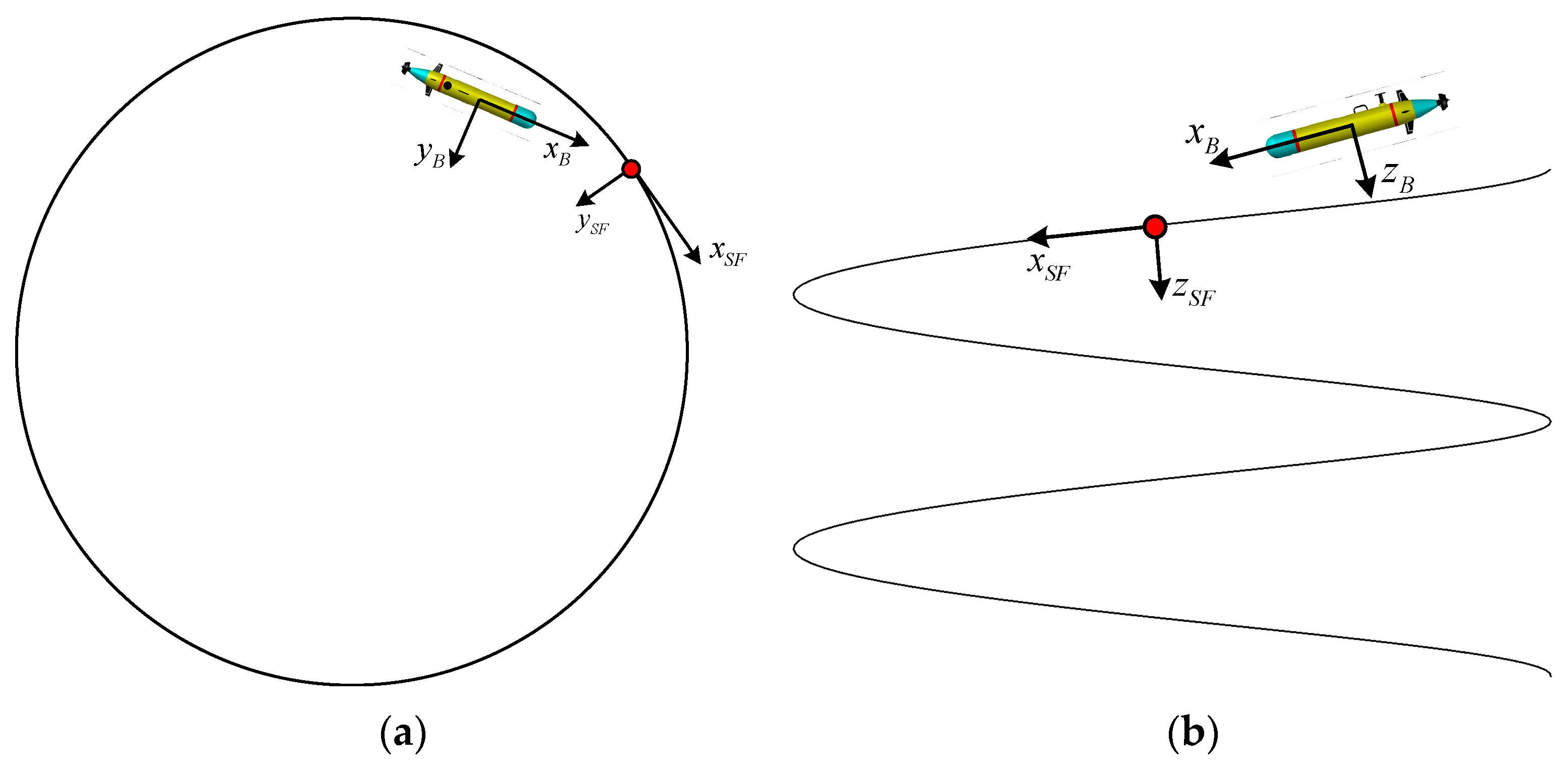
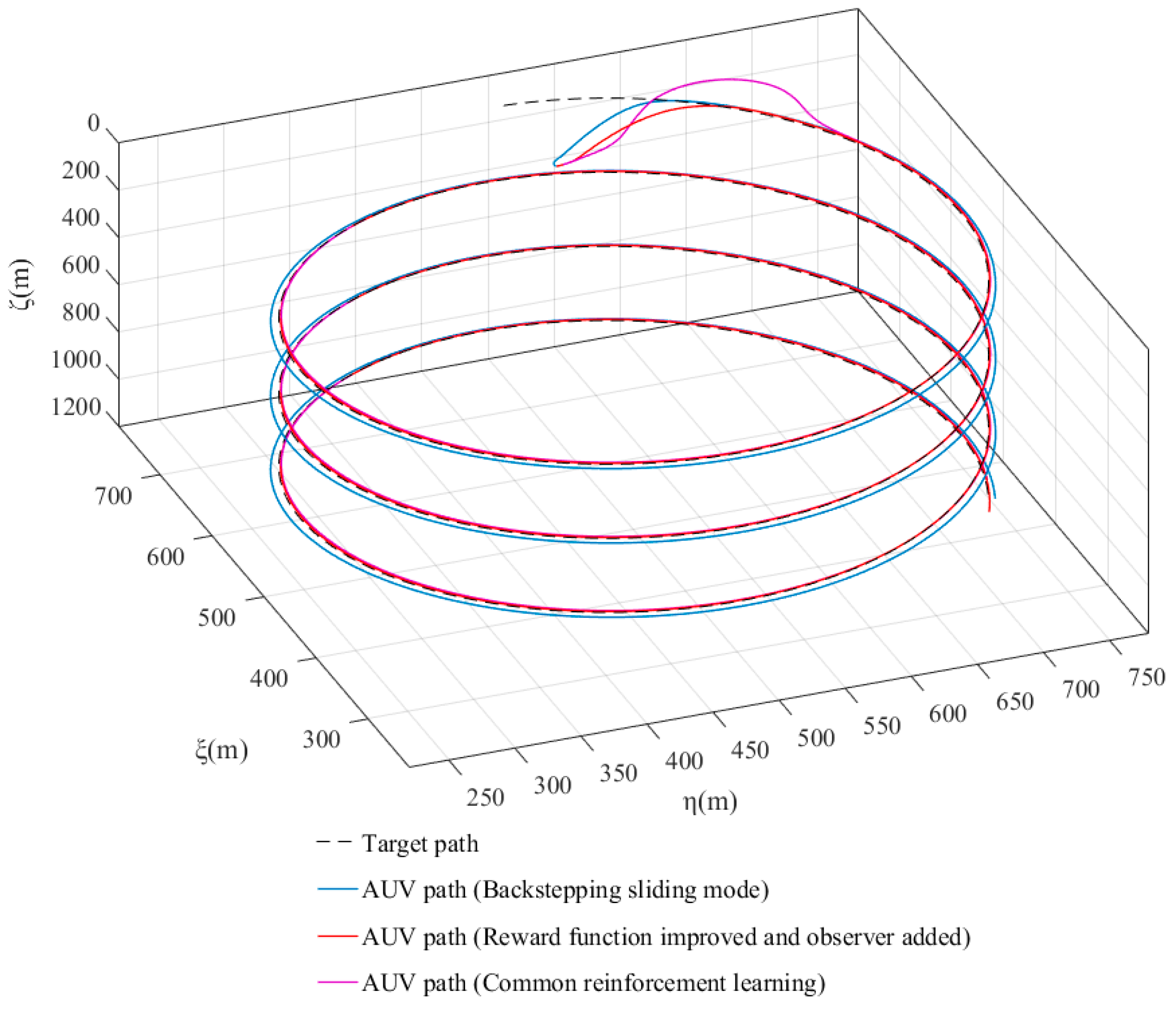
Combined with the improved line-of-sight method, the DDPG controller is designed. The guiding method using virtual AUV is researched and long-term stable path tracking is carried out successfully.

2. Modeling and Theory

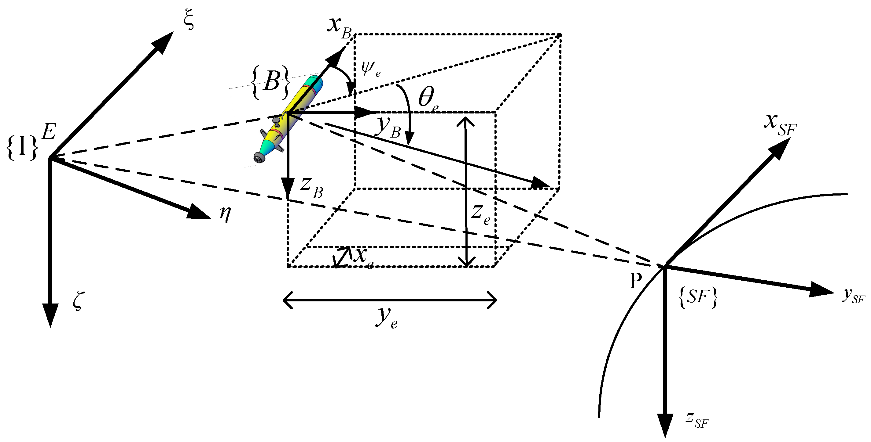
2.1. Coordinate System and Parameter Definition

In order to establish kinematics and dynamics models of AUV and the models of tracking errors, three coordinate systems were adopted: Geodetic coordinate system $\left\{I\right\}$, Carrier coordinate system $\left\{B\right\}$, and Curve coordinate system on the tracking path $\left\{SF\right\}$. The coordinate systems are shown in Figure 1.

$\left\{I\right\}$ is a geodetic coordinate system. The origin of the coordinate is set on the sea level. The $\xi$ axis points to the north, the $\eta$ axis points to the east, the $\zeta$ axis points to the center of the earth, and the $\xi$ axis, $\eta$ axis, and $\zeta$ axis form a right-handed coordinate system. $\left\{B\right\}$ is a carrier coordinate system. The origin of the coordinate $\left\{B\right\}$ is the AUV‘s center of gravity $Q$, the axis $x_B$ points to the AUV forward direction, the axis $y_B$ points to the starboard side of the AUV, and the axis $x_B$, axis $y_B$ and axis $z_B$ form a right- handed coordinate system; $\left\{SF\right\}$ is a Serret-Frenet coordinate system, the origin of the coordinate system $\left\{SF\right\}$ is set as point $s$ on the target path, and $s$ is the path parameter. The axis $x_{SF}$ is tangent to the path, $z_{SF}$ points downwards and is perpendicular to $x_{SF}$ and the plane defined by $x_{SF}$ and $z_{SF}$ is vertical. ${\psi }_p$ and ${\theta }_p$ are the attitude angles of the coordinate system $\left\{SF\right\}$ relative to the geodetic coordinate system $\left\{I\right\}$ [2,19]. ${\dot{\psi }}_p=c_1(s)\dot{s}$,${\dot{\theta }}_p=c_2(s)\dot{s}$, where:

$$\begin{gathered} c_1(s)=\frac{\left|{\dot{\xi }}_p(s){\ddot{\eta }}_p(s)-{\ddot{\xi }}_p(s){\dot{\eta }}_p(s)\right|}{{\left[{\left({\dot{\xi }}_p(s)\right)}^2+{\left({\dot{\eta }}_p(s)\right)}^2\right]}^{\raisebox{1ex}{$3$}\!\left/ \!\raisebox{-1ex}{$2$}\right.}} \\ {c}_2(s)=\frac{\left|{\dot{\xi }}_p(s){\ddot{\zeta }}_p(s)-{\ddot{\xi }}_p(s){\dot{\zeta }}_p(s)\right|}{{\left[{\left({\dot{\xi }}_p(s)\right)}^2+{\left({\dot{\zeta }}_p(s)\right)}^2\right]}^{\raisebox{1ex}{$3$}\!\left/ \!\raisebox{-1ex}{$2$}\right.}} \end{gathered}$$

2.2. AUV Model

The AUV three-dimensional motion model is presented in this chapter by reference to Fossen’s book [20]. The origin of the hull coordinate system was set at the AUV’s center of gravity, and we assumed the center of gravity and buoyancy to be in line with each other. Due to the good symmetrical structure AUV, the influence of the roll was ignored [21]. Therefore, the 6-DOF (degree of freedom) motion model can be simplified to a 5-DOF motion model. The kinetic equation of AUV is:

$$\{\begin{array}{l}(m-X_{\dot{u}})\dot{u}=X+f_u+X_{u\left|u\right|}u\left|u\right|+X_{uu}{u}^2+X_{vv}{v}^2+X_{ww}{w}^2+X_{qq}{q}^2\\ (m-Y_{\dot{v}})\dot{v}=f_v-(m-Y_r)ur+Y_{v}uv+Y_{v\left|v\right|}v\left|v\right|\\ (m-Z_{\dot{w}})\dot{w}=f_w-(m-Z_q)uq+Z_{w}uw+Z_{w\left|w\right|}w\left|w\right|+m{z}_g{q}^2\\ (I_y-M_{\dot{q}})\dot{q}=M+f_q+M_{q\left|q\right|}q\left|q\right|-M_{q}uq-M_{w}uw-\\ (z_{g}w-z_{b}B)\sin \theta -m{z}_g(wq-vr)\\ (I_z-N_{\dot{r}})\dot{r}=N+f_r+N_{v}uv+N_{v\left|v\right|}v\left|v\right|+N_{r}ur\end{array}$$

(1)

The dimensionless parameters used in this article are shown in

Table 1. Parameters in kinetic equation.

Mass Coefficients	$m=44.1\mathrm{kg}$	$I_y=8.0980\mathrm{kg}\cdot {\mathrm{m}}^2$	$I_z=8.0670\mathrm{kg}\cdot {\mathrm{m}}^2$
Hydrodynamic Added Mass Coefficients	${X_{\dot{u}}}^{\prime }$ = −0.00158	${Y_{\dot{v}}}^{\prime }$ = −0.030753	${Z_{\dot{w}}}^{\prime }$ = −0.0308
	${M_{\dot{q}}}^{\prime }$ = −0.001597	${N_{\dot{r}}}^{\prime }$ = −0.0016
Viscous Damping Coefficients	${X_{uu}}^{\prime }$ = −0.0059	${X_{vv}}^{\prime }$ = 0	${X_{ww}}^{\prime }$ = 0
	${X_{qq}}^{\prime }$ = −0.000985	${Y_r}^{\prime }$ = 0.0222	${Y_v}^{\prime }$ = −0.0450
	${Y_{v\left|v\right|}}^{\prime }$ = −0.1668	${Z_q}^{\prime }$ = −0.0171	${Z_w}^{\prime }$ = −0.0427
	${Z_{w\left|w\right|}}^{\prime }$ = −0.1297	${M_{q\left|q\right|}}^{\prime }$ = −0.00114	${M_q}^{\prime }$ = −0.01021
	${M_w}^{\prime }$ = 0.0103	${N_v}^{\prime }$ = −0.0094	${N_{v\left|v\right|}}^{\prime }$ = −0.0069
	${N_r}^{\prime }$ = −0.0117	$X_{u\left|u\right|}=-0.0725$
Shape Parameters	$L=1.46\mathrm{m}$	$d=0.21\mathrm{m}$

.

The kinematics equation of AUV is:

$$\{\begin{array}{l}\dot{x}=u\cos \psi \cos \theta -v\sin \psi +w\cos \psi \sin \theta \\ \dot{y}=u\sin \psi \cos \theta +v\cos \psi +w\sin \psi \sin \theta \\ \dot{z}=-u\sin \theta +w\cos \theta \\ \dot{\theta }=q\\ \dot{\psi }=r/\cos \theta \end{array}$$

(2)

where $m$ is the mass of AUV, $I_y$ and $I_z$ are the moments of inertia around the axis $y$ and axis $z$; $u$ is the velocity in the axis in an $x_B$ direction, $v$ is the velocity in the axis in a $y_B$ direction and $w$ is the velocity in the axis in a $z_B$ direction; $q$ is the velocity of pitch angle and $r$ is the velocity of the yaw angle; $X_{(\cdot )}$, $Y_{(\cdot )}$, $Z_{(\cdot )}$, $M_{(\cdot )}$, and $N_{(\cdot )}$ are the hydrodynamic coefficients of AUV. $z_g$ and $z_b$ are the positions of the center of gravity and the center of buoyancy in the hull coordinate system. $X$ is the longitudinal thrust generated by the propeller. $M$ and $N$ are the force moments around the $y_B$ axis and axis $z_B$, generated by the combined action of the propeller and rudders. In this article, the AUV is equipped with a pair of vertical rudders and a pair of horizontal rudders to control yaw and pitch, respectively. In general, the vertical rudders angle is set to positive when vertical rudders turn to starboard, and the horizontal rudders angle is set to positive when horizontal rudders turn to hull bottom. The mathematical model of the vertical rudder is:

$${\delta }_{r,real}=\{\begin{array}{l}{\dot{\delta }}_{r}t-{\delta }_{r,\max }<{\dot{\delta }}_{r}t<{\delta }_{r,\max }\\ {\delta }_{r,\max }{\dot{\delta }}_{r}t>{\delta }_{r,\max }\\ -{\delta }_{r,\max }{\dot{\delta }}_{r}t<-{\delta }_{r,\max }\end{array}$$

(3)

$${\dot{\delta }}_r={\delta }_{r,\max }/T_r$$

(4)

$${\delta }_{s,real}=\{\begin{array}{l}{\dot{\delta }}_{s}t-{\delta }_{s,\max }<{\dot{\delta }}_{s}t<{\delta }_{s,\max }\\ {\delta }_{s,\max }{\dot{\delta }}_{s}t>{\delta }_{s,\max }\\ -{\delta }_{s,\max }{\dot{\delta }}_{s}t<-{\delta }_{s,\max }\end{array}$$

(5)

$${\dot{\delta }}_s={\delta }_{s,\max }/T_s$$

(6)

• ${\delta }_{r,real}$: Actual vertical rudders angle.
• ${\delta }_{s,real}$: Actual horizontal rudders angle.
• $T_s,T_r$: Time constants of steering engines.

Rudder force and force moment are produced by the fluid acting on the rudder blade. The calculation of rudder force and force moment is complicated, which is related to aspect ratio, rudder area, rudder height, pitch propeller, and so on. By simplifying, the pitch force moment and yaw force moment are:

$$M=\frac{1}{2}\rho L^4{M}_{\left|q\right|{\delta }_s}^{\prime }u\left|q\right|{\delta }_s+\frac{1}{2}\rho L^3{M}_{{\delta }_s}^{\prime }{u}^2{\delta }_s$$

(7)

$$N=\frac{1}{2}\rho L^4{N}_{\left|r\right|{\delta }_r}^{\prime }u\left|r\right|{\delta }_r+\frac{1}{2}\rho L^3{M}_{{\delta }_r}^{\prime }{u}^2{\delta }_r$$

(8)

$M_{(\cdot )}^{\prime },N_{(\cdot )}^{\prime }$: Dimensionless hydrodynamic damping coefficients.

$\psi$ is the course angle of the AUV, $\theta$ is the flight path angle of AUV. The $v_t$ is the speed of the AUV:

$$v_t=\sqrt{u^2+v^2+w^2}$$

(9)

The point P is a dynamic point on the target path $\Gamma (s)$. In order to construct tracking target and get control errors, a virtual AUV was set on the target path $\Gamma (s)$. The point $p$ can be regarded as the center of gravity of the virtual AUV. The ${\psi }_p$ and ${\theta }_p$ are the attitude angles of the virtual AUV, and $V_p$ is the speed of the virtual target AUV. The kinematic equations of the virtual AUV are:

$$\{\begin{array}{l}{\dot{x}}_p=u_p\cos {\psi }_p\cos {\theta }_p-v_p\sin {\psi }_p+w_p\cos {\psi }_p\sin {\theta }_p\\ {\dot{y}}_p=u_p\sin {\psi }_p\cos {\theta }_p+v_p\cos {\psi }_p+w_p\sin {\psi }_p\sin {\theta }_p\\ {\dot{z}}_p=-u_p\sin {\theta }_p+w_p\cos {\theta }_p\\ {\dot{\theta }}_p=\gamma \\ {\dot{\psi }}_p=\omega \end{array}$$

(10)

We convert the error positions of the real AUV and virtual target AUV from the inertial coordinate system to the coordinate system $\left\{SF\right\}$:

$$\{\begin{array}{l}{x}_e=(x-x_p)\cos {\psi }_p\cos {\theta }_p+(y-y_p)\sin {\psi }_p\cos {\theta }_p-(z-z_p)\sin {\theta }_p\\ y_e=-(x-x_p)\sin {\psi }_p+(y-y_p)\cos {\psi }_p\\ z_e=(x-x_p)\cos {\psi }_p\sin {\theta }_p+(y-y_p)\sin {\psi }_p\sin {\theta }_p+(z-z_p)\cos {\theta }_p\end{array}$$

(11)

Differentiating on both sides of the Equation (11), and substitute it into the Equations (2) and Equation (10). The equation of dynamic error is:

$$\{\begin{array}{l}{\dot{x}}_e=y_e{c}_1(s)\dot{s}\cos {\theta }_p-z_e{c}_2(s)\dot{s}+v_t\cos {\psi }_e\cos {\theta }_e-\dot{s}\\ {\dot{y}}_e=-x_e{c}_1(s)\dot{s}\cos {\theta }_p-z_e{c}_1(s)\dot{s}\sin {\theta }_p+v_t\sin {\psi }_e\cos {\theta }_e\\ {\dot{z}}_e=x_e{c}_2(s)\dot{s}+y_e{c}_1(s)\dot{s}\sin {\theta }_p+v_t\sin {\theta }_e\end{array}$$

(12)

2.3. Deep Reinforcement Learning Theory

The reinforcement learning problem is how to achieve a goal or accomplish a control task through constant interactions in real or simulated system. RL formulations of the control problem contain four elements in general: state space, action space, probability of state transition, and reward function. The objective of the artificial agent is to get an optimal policy for a specific problem, so that the reward obtained from the strategy is the largest, that is, optimal action, can be selected in different system states. During the learning process, an artificial agent interacts with the system by taking an action, which is chosen from the action space. Then, the artificial agent will receive a signal call reward, which deliver a measure of how good or how bad the action taken according to the observed state transition [22]. Regardless of whether the reward is good or bad, it will make the next selected action more likely to produce a better state transition.

The goal in reinforcement learning is to learn a policy that maximizes the expected return $J$ from the start distribution [9]:

$$J=E_{R_i,s_i~E,a_i~\pi }[R_1]$$

(13)

where $R_1$ is the discounted sum of rewards. A common model of reinforcement learning is a standard Markov Decision Process (MDP), which is used to describe and solve how agents can maximize their rewards or achieve specific goals through learning strategies in their interactions with the environment. The MDP is based on the Markov stochastic process, which indicates that in a random process, the state at the next moment is only related to the current state, regardless of the previous state [23]. A Markov decision process M on a set of states $S$ and with actions $\left\{a_1,...,a_k\right\}$ consists of:

Transition probabilities: for each state-action pair $\left(s_t,a\right)$, $P_{s_t,a}(s_{t+1})$ denotes the probability of transiting from $s_t$ to $s_{t+1}$ on taking action $a$:

$$P_{s_t,a}(s_{t+1})=P(s_{t+1}|s_t,a)\forall i,j\ge 0$$

(14)

Reward distributions: for each state-action pair $\left(s_t,a\right)$, a distribution $r_{sa}$ on real-valued rewards for executing action $a$ from state $s_t$:

$$r_{sa}=r(s_t,a,s_{t+1})$$

(15)

where $S$ is a finite set of state, with a distinguished initial state $s_0$, and A is a finite set of actions:

$$S=\{s_0,s_1,s_2\dots \}$$

(16)

$$A=\{a_1,a_2,a_3\dots \}$$

(17)

In MDP, the policy is a conditional probability distribution of actions basing on state, and the policy decision can be written as:

$$\pi (a|s)=p(a|=s)$$

(18)

The action-value function is used in many reinforcement learning algorithms. It describes the expected return after taking an action $a_t$ in state $s_t$, and thereafter, following policy π:

$$Q^{\pi }(s_t;a_t)=E_{ri\ge t,si>t\sim E,ai>t\sim \pi }[R_t|s_t,a_t]$$

(19)

$$R_t={\displaystyle {\sum }_{i=t}^T{\gamma }^{(i-t)}}r(s_t,a_t)$$

(20)

where $\gamma \in [0,1]$ is a discount factor. A path $\chi$ of an MDP is a nonempty sequence:

$$\chi =s_0\stackrel{a_0}{\to }{s}_1\stackrel{a_1}{\to }{s}_2\dots s_i\stackrel{a_i}{\to }{s}_{i+1}$$

(21)

Deep neural networks refer to those networks organized in in depth architectures, as in mammal brains. The purpose of applying deep neural networks is to accurately find a description of the characteristics of things, so as to make the correct classification. Recently, deep neural networks have arisen as a way to deal with large data sets for applications in classification and regression. Optimal policy can be stored in a deep neural networks. Deep neural network architectures are able to transform a high dimensional input data into a reduced output feature, and the parameters of the networks are learned applying backpropagation algorithms. After the training progress accomplished, the system state will be entered into the neural network, and the control signals will be output from the neural network for path tracking.

The artificial agent in deep reinforcement learning understands the world slowly and learns how to accomplish a task by repeated attempts. External feedback and actions valuing reward and punishment were used to update the parameters of the networks in the process of deep reinforcement learning for AUV path tracking, making the next AUV instruction more likely to produce the desired results. The motion commands are generated from the neural networks, thus, the process of deep reinforcement learning can be seen as a process of continuously updating the neural network parameters [24].

The main goal in this article is to design a DDPG-based training method for controller, and to carry out a path tracking simulation successfully. At the same time, the anti-disturbance ability, tracking performance and steering efficiency of the AUV should be improved as much as possible.

3. Tracking Control Method and Deep Deterministic Policy Gradient Algorithm

In order to provide a guide for AUV, the coordinate system $\left\{SF\right\}$ was designed, and the virtual AUV can be considered as a target point. The position of the virtual AUV on the target path was determined by a path parameter whose derivative was taken as:

$$\dot{s}=k_3{x}_e+U_B\cos {\psi }_e\cos {\theta }_e$$

(22)

where $U_B\cos {\psi }_e\cos {\theta }_e$ is the projection of the velocity of the robot on the $x_{SF}$. In this way, the virtual AUV can always stay ahead of the AUV, not too far away or behind. The virtual AUV provides the AUV with a target. The path parameter $s$ can be obtained through integral transformation.

The concept of guidance angles in [25] was introduced, which was used to provide target errors of angles for AUV and avoid the movement locus of the AUV parallel to the target path. In fact, horizontal guidance angle $\delta (y_e)$ is the expectation of course angle error ${\psi }_e$, vertical guidance angle $\chi (z_e)$ is the expectation of flight path angle error ${\theta }_e$. The design of the guidance angle should meet the following conditions:

(1)

$\delta (0)=0$

(2)

$y_e\delta (y_e)\ge 0$

(3)

$\chi (0)=0$

(4)

$z_e\chi (z_e)\ge 0$

The guidance angles were designed as:

$$\delta (y_e)=-{\psi }_a\frac{e^{2k_{\psi }{y}_e}-1}{e^{2k_{\psi }{y}_e}+1}{\theta }_a>0$$

(23)

$$\chi (z_e)=-{\theta }_a\frac{e^{2k_{\theta }{z}_e}-1}{e^{2k_{\theta }{z}_e}+1}{\psi }_a>0$$

(24)

$${\epsilon }_{\psi }={\psi }_e-\delta (y_e)$$

(25)

$${\epsilon }_{\theta }={\theta }_e-\chi (z_e)$$

(26)

$\delta (y_e)$ is a monotonic minus function, and its curve goes through the origin. ${\theta }_a>0$; the algorithm’s purpose is to make ${\epsilon }_{\psi }$ and ${\epsilon }_{\theta }$ as close to 0 as possible. Thus, when $y_e>0$, as the expectation of course angle error, we make $\delta (y_e)<0$, which leads to ${\psi }_e<0$. That can be explained as we hope that the angle between $x_B$ and $x_{SF}$ is less than 0 when AUV is on the right side of the point $P$, so that the AUV will turn left and move forward to target path. For the same reason, when $y_e<0$, $\delta (y_e)>0$. The AUV will be guided to turn right and move toward the target path. As for the vertical plane, $\chi (z_e)$ will lead AUV rise and dive by similar process. The AUV will be always guided to the target path through this mechanism. By applying the guidance angles, the path length of the AUV can be shortened and the energy can be saved. AUV will be better with endurance and long-distance.

The AUV in this article is operated by a main propeller, horizontal rudders, and vertical rudders. Therefore, there are three outputs from the AUV controller: forward thrust, vertical rudders angle and horizontal rudders angle. Here, we applied a Deep Deterministic Policy Gradient (DDPG) [17]. This policy refers to the behavior of the agent, which is a mapping from state to action and the conditional probability distribution of the action. DDPG is derived from the improved Actor-Critic, which combines the advantages of Policy-based Policy Gradients and value-based Q-learning learning methods. Therefore, DDPG can learn from continuous motion distribution, and meeting the characteristics of AUV-driven actuators. DDPG also absorbs the advantages of DQN, using replay buffer to store samples. Then, a certain amount of data are randomly selected for learning, effectively reducing the continuity of the state in the learning data [26].

There are two types of neural networks in DDPG: actor network and critic network, which correspond to deterministic policy and action-value function [9]. For the actor network, the actor function $\mu \left(s|{\theta }^{\mu }\right)$ maps states to a specific action, and the estimated networks is used to output real-time actions for actors to perform in real environment. The actor is updated by following the applying the chain rule to the expected return from the start distribution $J$ with respect to the actor parameters ${\theta }^{\mu }$:

$${\nabla }_{{\theta }^{\mu }}J\approx E_{s_t\sim {\rho }^{\beta }}[{\nabla }_{a}Q\left(s_t,a|{\theta }^Q\right){|}_{s=s_t,a=\mu (s_t)}{\nabla }_{{\theta }_{\mu }}\mu (s|{\theta }^{\mu }){|}_{s=s_t}]$$

(27)

where $\beta$ is stochastic behavior policy. We denote the discounted state visitation distribution for a policy $\beta$ as ${\rho }^{\beta }$. We consider action-value function approximators parameterized by ${\theta }^Q$. The action-value function $Q^{\pi }\left(s_{t,}{a}_t\right)$ describes the expected value after taking an action $a_t$ in state $s_t$ and following policy $\pi$.

$$Q^{\pi }\left(s_{t,}{a}_t\right)=E_{r_{i\ge t},s_{i>t}\sim E,a_{i>t}\sim \pi }[R_t|s_t,a_t]$$

(28)

where $R_t$ is the sum of discounted future reward.

The critic networks of DDPG is optimized by minimizing the loss function:

$$L\left({\theta }^Q\right)=E_{s_t\sim {\rho }^{\beta },a_t\sim \beta ,r_t\sim E}[{(Q(s_t,a_t|{\theta }^Q)-y_t)}^2]$$

(29)

where:

$$y_t=r(s_t,a_t)+\gamma Q\left(s_{t+1},\mu \left(s_{t+1}\right)|{\theta }^Q\right)$$

(30)

The process of the neural network parameters update in the two systems is shown in the Figure 2.

The value-based part is shown in the left-hand dotted box, and the policy-based part is shown in the right-hand dotted box. The critic networks are used to approximate the optimal policy, the ability to select actions which can bring the highest value in different states. The evaluation networks in critic networks are used to update the value-based networks and calculate the value of the current action. The target networks are used to analyze the observed value and the action outputted from the target networks of the actor networks.

The actor networks are used to output actions under supervision of the critic networks. In actor networks, the evaluation networks are used to output real-time actions and update the policy-based networks. The outputs of the target networks are used to select the best next action for updating critic networks. The meaning of each letters is:

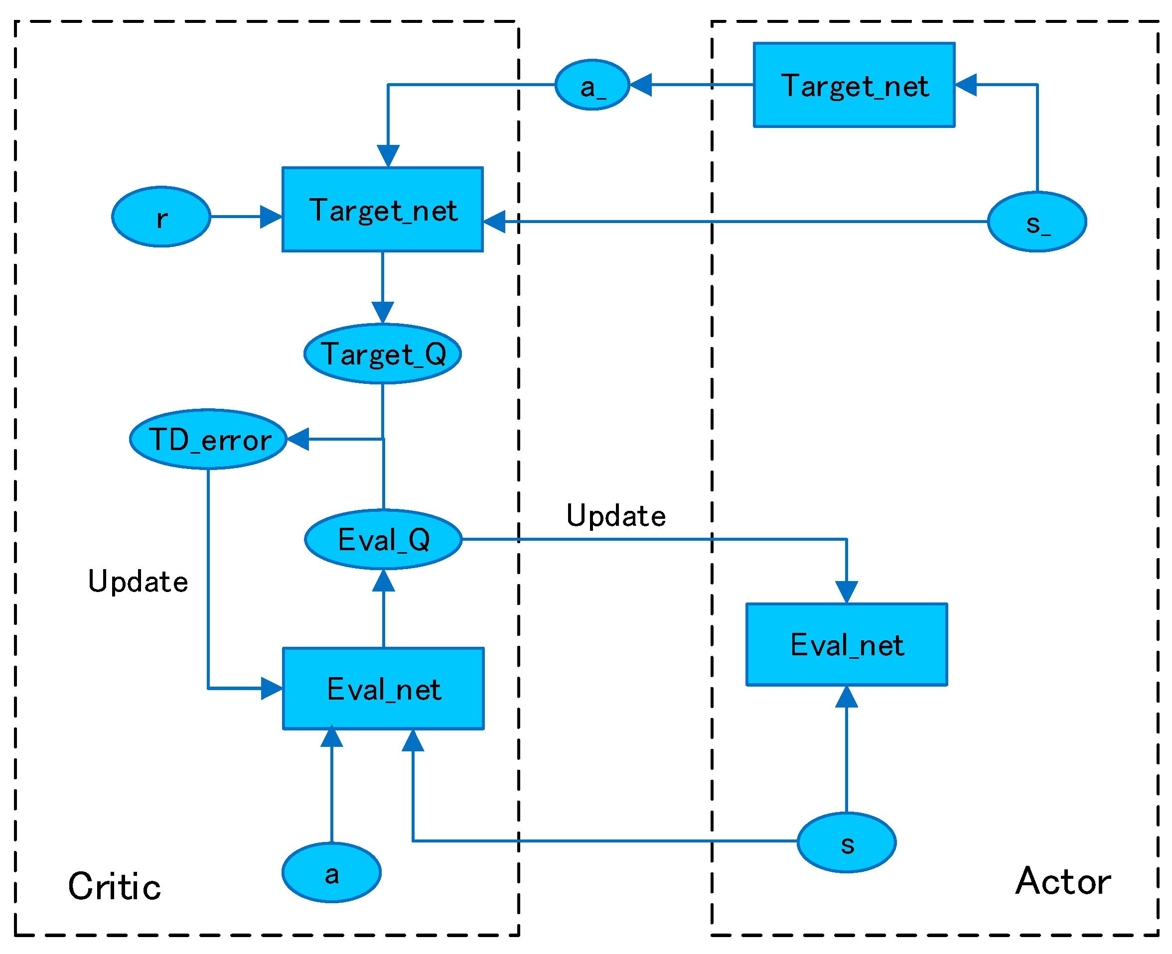
• s: Current state
• s_: State of the next moment
• a: Current action
• a_: Next action
• r: Reward
• Target_Q: The target value calculated by the next state_s, the estimated value of the predicted action a_, and the reward value.
• Eval_Q: The current value obtained by importing the current state and current action into Eval_net.
• TD_error: The difference between target_q and eval_q, which is used to backpropagate to approach the parameters.

In the critic neural networks, estimated value of action Q_ was obtained by importing the next state (s_) and the next action (a_) into the state estimation network. The Q_target can be also obtained after the current reward added. The parameters of the critic are updated in the process of minimizing TD_error, so as to accomplish accurate value judgment. In the update of the actor neural network, the Eval-net parameters in the actor were updated in the process of maximizing Eval_Q.

The reward function contains the current AUV state was set:

$$R=-\sqrt{{\epsilon }_{\psi }^2+{\epsilon }_{\theta }^2+u_e^2}$$

(31)

In order to test the path tracking effect based on deep reinforcement learning suggested in this article, we implemented DDPG basing on previous work. A deep reinforcement learning environment was built basing on Python, the training scene was designed, and a high-speed autonomous underwater vehicle was adopted as the test subjects. The motion control actuators of the AUV include a stern thruster, a pair of horizontal rudders, and a pair of vertical rudders. TensorFlow was applied to build Neural Networks and accomplish the process of Parameters’ update in deep reinforcement learning. The dimension of the environmental state space was set to 6, which included error of the course angle, error of the flight path angle, error of the speed, and the distance between the AUV and the virtual AUV in the three coordinate axes. The dimension of the action space was set to 3; the actions included the yaw force moment, the pitching force moment, and the forward thrust. The learning rate for actor network and the learning rate for critic network were both set to 0.001. Of course, in order to maximize the total reward from the current moment until the state reaches the goal and reduce the impact of future reward on current actions, the reward discount $\gamma$ was set to 0.9.

There are two layers in the actor networks in this article. The input of first layer is state, and there are 300 neurons included, while the activation function is rectified linear unit (ReLU) function. Corresponding to the dimension of the action, the number of neurons of the second layer is 3. The activation function of the second layer is tanh function. There is one layer in critic networks. The input is the value of ReLU function which contains state and action, as the output is value Q.

During training of the intelligent agent in the simulation, the iterations was set to 1000. The intelligent agent was reset to the initial state at the beginning of the each episode, and superposition of rewards was reset to 0 at the same time. The episode length was set to 2000, which means that the process of selecting action, state transition, and calculation of the reward value will be performed 2000 times in each episode. The results were stored in the replay buffer after 1000 episodes of training, and 32 sets of data were randomly extracted for parameter updating each time. When the iterations reach 1000 and the average of the last 100 rewards is greater than −40, the reinforcement learning process will stop. Otherwise, another 1000-step iteration will continue to be performed. The latest policy will be chosen as the control law.

Most optimization algorithms assume that the samples are independently and identically distributed. However, this assumption no longer holds true, as our samples are generated from exploring sequentially in an environment. Moreover, replay buffer, which is a finite sized cache, was used to address these issues. We reserved 40,000 units of space for replay buffer. The samples include the state before the performance, the action being performed, the reward of the current action, and the state after the action is performed. When the replay buffer is full, the old samples would be replaced by new samples.

In addition, an exploration parameter $\epsilon =5$ was set to add randomness to action selection for exploration during training. As is shown in Figure 3, after an action $a$ output from the Actor networks, a normal distribution will be constructed, whose average value is $a$. A new action $a^{\prime }$ will be selected from the interval $\left[a-\epsilon ,a+\epsilon \right)$ by following normal distribution. Moreover, every time the neural network parameters are updated, $\epsilon$ will be self-multiplied by 0.995 to gradually reduce exploratory action selection as learning progresses.

4. Simulation and Improvement

4.1. Preliminary Simulation Experiment

Considering the dive process above, a cylindrical helix path was used to test the path tracking performance of deep reinforcement learning controller. In the process of the cylindrical helix path tracking, it is obvious that the desired velocity of course angle and the desired flight path angle are constant values, but we still believe that it can continuously train and optimize the controller. This is because the reward function we selected was not only related to the states, but also included the errors of angles based on the improved line of sight (LOS) method. The target of training is not only to maintain a specific angle or velocity of angle, but to approach the dynamic horizontal and vertical guidance angles that are related to the changing states. As a goal, training with a cylindrical helix path is representative, and we believe the trained path tracking controllers can be applied to other environments and other tracking paths effectively. The parametric equation of the path is:

$$\{\begin{array}{l}\xi (s)=250\cos \left(s\right)+500\\ \eta (s)=250\sin \left(s\right)+500\\ \zeta (s)=50s+50\end{array}$$

(32)

The initial position of the virtual AUV is $S(0)=0$, the initial position of the AUV is $\xi (0)=650$, $\eta (0)=500$, and $\zeta (0)=50$, the initial course angle is $\psi (0)=0$, and the initial flight path angle is $\theta (0)=0$. Initial speed is 0.1 m/s, expected forward speed is $u_d=6$ m/s. Disturbance water currents are added into the environment. In the inertial coordinate system, the water flow has a velocity of 0.3 m/s in the $\xi$ direction, 0.3 m/s in the $\eta$ direction, and 0.15 m/s in the $\zeta$ direction. The training scene is shown in the Figure 4.

The reinforcement learning environment and methods in Section 3 was used to train the path tracking controller. Then, a motion simulation was carried out for 10,000 steps; the simulation results are shown in the following Figure 5, Figure 6 and Figure 7.

It can be clearly seen from Figure 6 and Figure 7 that the AUV path tracking succeeded as a whole. In the 10,000-step episode, the average of distance between the AUV position and the target position was 5.5 m. However, in the initial stages, because the controller was not sensitive enough, there was a large overshoot. The maximal error in the $\xi$ direction reached 36 m, while the maximal error in the $\eta$ direction reached 30 m. Moreover, due to the water currents, the AUV oscillated on both sides of the target path, and there were static errors. The range of the horizontal rudders angle is from −16° to 16°, and range of the vertical rudders angle from −16° to 16°. It can be seen from Figure 7 that during the simulation test, the average value of the horizontal rudder angle was −0.545°, the variance was 4.09°, the average value of the vertical rudder angle was 3.00°, and the variance was 9.14°. The rudder angle continued to be at a maximum for a long period of time, and the rudder angle changed frequently. That may lead to the low efficiency of steering and increasing useless consumption of energy.

The reinforcement learning reward curve in 1000 episodes of path tracking is shown in Figure 8. The value of each point in the Figure 8 was accumulated by the reward values in each episode.

Due to the Policy Gradient in the DDPG reinforcement learning algorithm, the neural network can be updated by learning in both successful and failed experiences. As can be seen from the reward value curve shown in the Figure 8, the reward value stable and high for most of the time, but there are low reward values from 600 to 700 steps. It shows that the neural network controller learned a lot in the successful experiences, but few in the failed experience. That may lead to the controller falls into local optimum and lacks exploratory. In order to approach success and avoid failure, good neural network controllers should be able to learn in both successful and failed experiences.

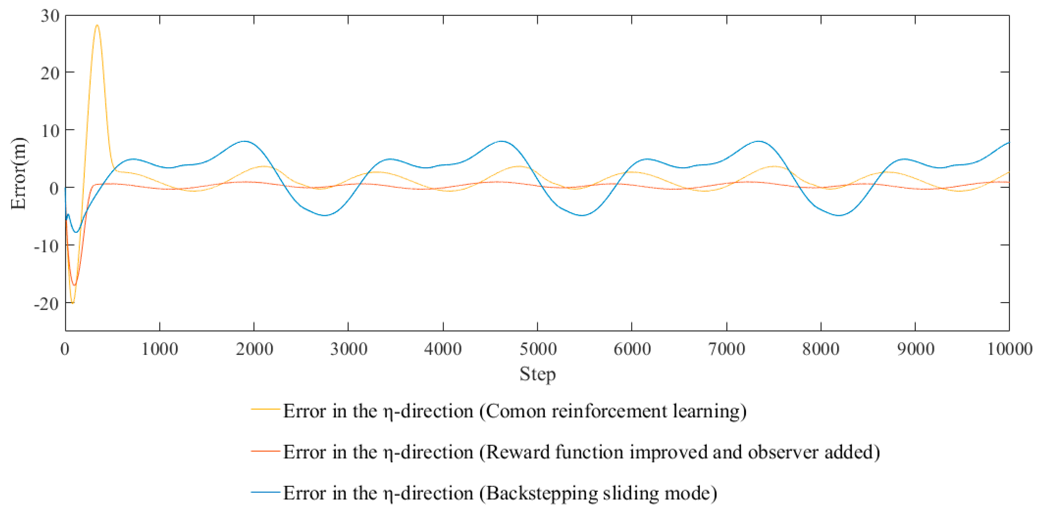
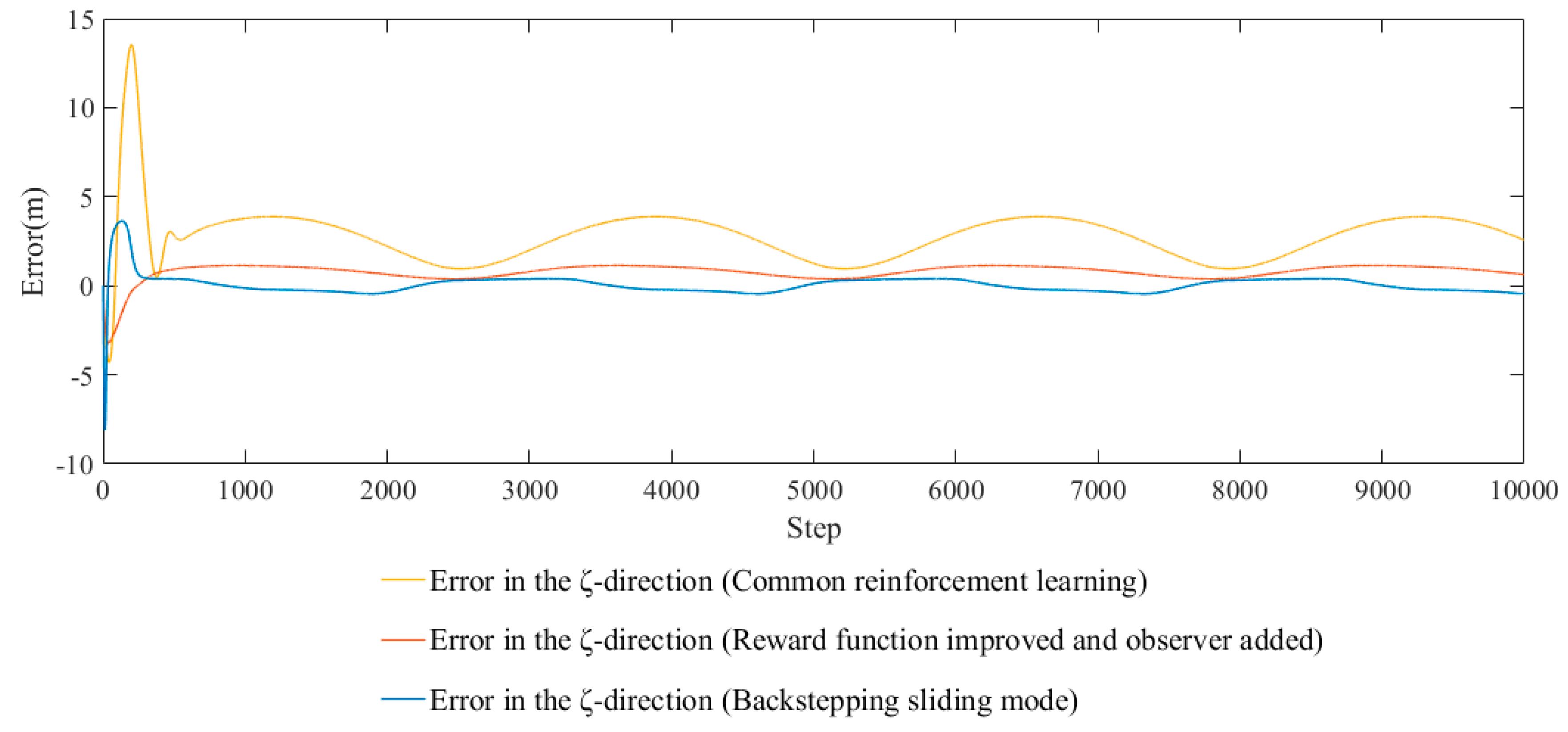
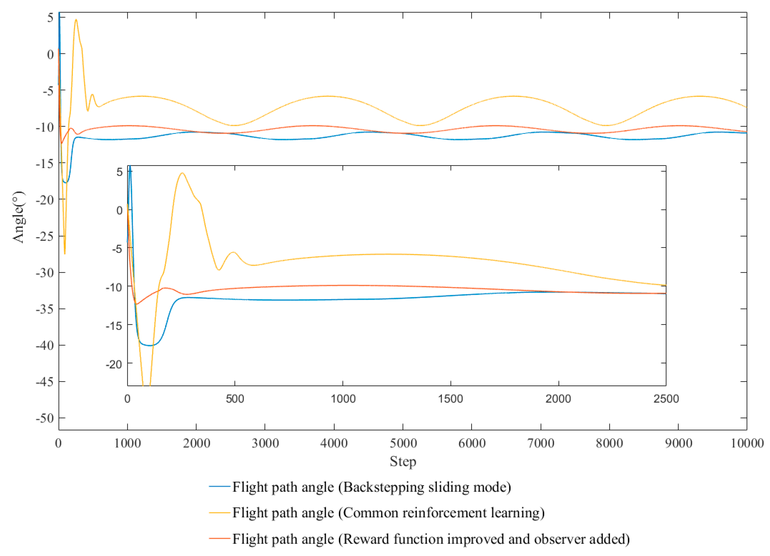
4.2. Improve

We made some improvements after analyzing the above simulation results. In order to avoid frequently changing of the rudders angle, penalty terms were added into reward function. The improved value function is:

$$R_l=k_1\left(e^{-\left({\delta }_r^2+{\dot{\delta }}_r^2\right)}-1\right)+k_2\left(e^{-\left({\delta }_s^2+{\dot{\delta }}_s^2\right)}-1\right)+k_3\sqrt{{\epsilon }_{\psi }^2+{\epsilon }_{\theta }^2+u_e^2}$$

(33)

where ${\delta }_r$ is the vertical rudders angle and ${\delta }_s$ is the horizontal rudders angle. The selections of weight coefficients $k_1,k_2,k_3$ are influenced by different models, environments, and objectives. Here, $k_1=0.3,k_2=0.2,k_3=0.5$.

The rudders angle and their rates of change were added into a deformed second-order Gaussian function to form the penalty terms. Moreover, a boundary reward function was proposed, as shown in the following equation:

$$R_b(x_e,y_e,z_e,{\psi }_e,{\theta }_e)=\{\begin{array}{l}1if\left|x_e\right|<5\cap \left|y_e\right|<5\cap \left|z_e\right|<5\cap \left|{\psi }_e\right|<0.4\cap \left|{\theta }_e\right|<0.2\\ 0otherwise\end{array}$$

(34)

A cube was presented, which is centered on the virtual AUV and has a side length of 5 m. If the errors of AUV’s flight path angle and course angle maintain small values, and the AUV’s position is within the range of cube, the reward value will be 1, otherwise 0. The final reward value is:

$$R=R_l+R_b$$

(35)

At the same time, in order to avoid local optimum in the learning process, reduce the continuity of the state in the learning data, we increased the size of the replay buffer from 40,000 units to 100,000 units. Moreover, an integral term was added into guidance angle to eliminate the periodic error. The errors change to:

$${\epsilon }_{\psi }={\psi }_e-\delta (y_e)+k_{\psi }{\displaystyle {\int }_0^t\left[{\psi }_e-\delta (y_e)\right]}dt$$

(36)

$${\epsilon }_{\theta }={\theta }_e-\chi (z_e)+k_{\theta }{\displaystyle {\int }_0^t\left[{\theta }_e-\chi (z_e)\right]dt}$$

(37)

Sharma and Verma proposed a wavelet neural network reduced order observer based adaptive tracking control strategy for a class of systems with unknown system dynamics. The wavelet adaptive reduced order observer was used to perform the task of identification of unknown system dynamics [27]. Xiangbin Wang proposed an adaptive disturbance observer for near-wall-following control [28]. In order address the problem of disturbance from currents. It was decided to add a disturbance observer into the control system, so that the controller output can be adjusted in real time according to the observed disturbance patterns and features. The basic idea of designing a disturbance observer is to correct the estimated value by measuring the difference between the estimated outputs and the actual outputs [29]. Therefore, the disturbance observer is designed as:

$$\begin{array}{l}\dot{\widehat{d}}=n_1\left(\widehat{\omega }-\dot{\vartheta }\right)\\ \dot{\widehat{\omega }}=-\widehat{d}+a\ell -n_2\left(\widehat{\omega }-\dot{\vartheta }\right)-b\dot{\vartheta }\end{array}$$

(38)

where $n_1$,$n_2$ are observer parameters, $\dot{\vartheta }$ is the derivative value of the current state, $\widehat{\omega }$ is the estimated value of $\dot{\vartheta }$, $\widehat{d}$ is the estimated value of the disturbance signal, $\ell$ is the controller output, $a$ and $b$ are parameters related to the model and tracking states. Since the tracking controller outputs three generalized forces, three disturbance observers were added. They are:

$$\{\begin{array}{l}{\dot{\widehat{d}}}_u=n_1\left({\widehat{\omega }}_u-\dot{u}\right)\\ {\dot{\widehat{\omega }}}_u=-{\widehat{d}}_u+a_u{\sigma }_u-n_2\left({\widehat{\omega }}_d-\dot{u}\right)-b_u\dot{u}\end{array}$$

(39)

$$\{\begin{array}{l}{\dot{\widehat{d}}}_q=n_1\left({\widehat{\omega }}_q-\dot{q}\right)\\ {\dot{\widehat{\omega }}}_q=-{\widehat{d}}_q+a_q{\sigma }_q-n_2\left({\widehat{\omega }}_q-\dot{q}\right)-b_q\dot{q}\end{array}$$

(40)

$$\{\begin{array}{l}{\dot{\widehat{d}}}_r=n_1\left({\widehat{\omega }}_r-\dot{r}\right)\\ {\dot{\widehat{\omega }}}_r=-{\widehat{d}}_r+a_r{\sigma }_r-n_2\left({\widehat{\omega }}_r-\dot{r}\right)-b_r\dot{r}\end{array}$$

(41)

The estimated value of the disturbance signals are input into the controller. The structure is shown in the Figure 9.

The disturbance was estimated by observing the outputs from the controller and the current states of the AUV. The inputs of the controller are virtual control signals, current states of the AUV, and the observer’s estimated value of the disturbance. It is equivalent to an anti-disturbance item $\widehat{d}$ was added directly into the controller.

After that, the reward function was improved and the current observer was added. We trained the new controller, and this trained controller was used for the simulation experiment. The results of the simulation were compared with the simulation experiment results before the improvements and the results of backstepping sliding mode controller [30], which are shown below. The path tracking performances of simulations which applying three kinds of different controllers are shown in the Figure 10. The red line represents the tracking path applying the deep reinforcement learning controller with new reward function, the yellow line corresponds to backstepping sliding mode controller, and the blue line corresponds to the previous deep reinforcement learning controller.

What is shown in Figure 11 are the position errors in the axis in a $\xi$ direction, which applies three different controllers. In Figure 11, the horizontal axis indicates the steps number of simulation iteration, and one step corresponding to 0.1 s. It can be seen from movements of the AUV that periodic errors in the $\xi$ direction also exist. Among them, the errors of simulation that apply the backstepping sliding mode controller are greater, and the maximum of errors reaches 7 m. The common deep reinforcement learning controller also presents obvious periodic error, there is an error of nearly 37 m in the initial stage, and then the error curve tends to be gentle. The reward function improved controller presents a maximal error nearly 8 m. There is no obvious periodic change after stabilization, and the performance is very stable.

The position errors in axis $\eta$ direction are shown in Figure 12. The errors of the simulation that apply the backstepping sliding mode controller are large, and the maximum reaches 8 m. The simulation applying the deep reinforcement learning controller presents errors of nearly 27 m in the initial stages, and the error curve tends to be gentle. The reward function improved controller presents a maximal error of about −17 m, and it tends to be gentle after the maximal error. There is no obvious periodic change after stabilization, and the performance is very stable.

The errors in the axis in a $\zeta$ direction in three simulations are shown in the Figure 13. Among them, the errors in the simulation that apply the backstepping sliding mode controller is large, and the maximum value reaches −8 m. The common deep reinforcement learning controller also presents obvious periodic errors, and there is an error of nearly 14 m in the initial stage before the error curve tends to be gentle. The maximum error of reward function improved controller is about 1 m, and the error curve tends to be gentle quickly.

The inputs of the disturbance observer are states and outputs from the controller, so the observer can adjust the controllers. Our other improvements mainly revolved around the optimization of reinforcement learning reward function, which should be effective in steering and learning efficiency. As can be seen from the Figure 11, Figure 12 and Figure 13, the periodic errors caused by water currents in three directions were all reduced. The disturbance observer presents a positive performance.

The course angles of simulations are shown in Figure 14. From the comparison of the three curves, it can be seen that the course angle curve corresponding to deep reinforcement learning is better than that corresponding to the back-stepping sliding mode controller. Moreover, the controller after the reward function improved presents an even better performance than before. The improved deep reinforcement learning controller takes less time before the course angle is stable.

The curve of flight path angle in simulations that apply three different kinds of controllers are shown in Figure 15. The maximum of the flight path angle corresponding to the backstepping sliding mode controller is about 5°; the minimum is about −18°. Then, it oscillates up and down at −12°. The common deep reinforcement network controller presents a maximum flight path angle of about 5°, a minimum of about −27°, and then periodically changes around −8°. After the reward function was improved, the maximum of the flight path angle is about 1°; the minimum is about −12°. After about 900 steps from the beginning, the curve starts to stabilize at −10°.

The vertical rudders angle curves and horizontal rudders angle curves of the simulations, which apply the two deep reinforcement learning controllers, are shown in Figure 16 and Figure 17. It can be seen that the horizontal rudders angle changes frequently when the reward function has not been improved. The rudders angle is generally large, and stays at its maximum in the initial stages. We can see from the curve of the simulation that by applying the improved controller, the absolute value and change rate of the horizontal rudders angle are greatly reduced, and the horizontal rudders angle finally stabilize at about −0.5°. Similarly, we can find from the curve of simulation that by applying the improved controller, the absolute value and the change rate of the vertical rudders angle are greatly reduced as well, and the vertical rudders angle finally stabilize at about 3°. Some statistics are shown in the

Table 2. Rudders angle statistics.

	Common Reinforcement Learning	Reward Function Improved and Observer Added
Average of horizontal rudders angle	−0.477°	−0.556°
Variance of horizontal rudders angle	3.13	0.27
Average of vertical rudders angle	3.00°	2.06°
Variance of vertical rudders angle	7.00	1.78

, the oscillations of the horizontal rudders angle and the vertical rudders angle are both reduced after applying the new reward function improved. It can be seen that the new controller improves the efficiency of steering, as the tracking performance is also improved.

When the iterations reach 1000 and the average of the last 100 rewards is greater than 300, the reinforcement learning process will stop. The reward curve of deep reinforcement learning in 1000 episodes for path tracking is shown in Figure 18. Since the data, such as the environmental states and the reward values, were stored in the replay buffer during the training of the neural networks, the update started only if the replay buffer was full, thus, there is a straight line at the start. It can be seen from the comparison that the new reward value curve continues to mutate and vibrate in the early stages, while the old reward value curve has fewer mutations and vibrations. That is because a new term about rudders angle and a boundary reward function were added into the reward value function, which makes the process of parameters update more complicated. However, that also avoided the update of the parameters being slowed due to the decrease of the reward value change rate; on the other hand, the enlarged replay buffer space enable more data to be stored, which reduced the possibility of falling into a local optimum, and enhanced the capacity to explore.

5. Conclusions

The analysis and modeling of AUV 3D path tracking problem were accomplished in a case study of a cylindrical helix path. The training environment for 3D path tracking was designed by applying deep reinforcement learning DDPG algorithm. A method of selecting actions based on positive distribution was adopted to maintain the exploratory action selection. The rudders angles and their rates of change was added to be the new term in reward function, and a boundary reward was also designed to form a part of the reward function. The new reward function was shown to be effective to lower the frequency of steering. The LOS method with the integral term added was adopted to provide an indication of the target course angle and target flight path angle. Furthermore, to enable the controller to observe the current disturbance and adjust outputs, a currents disturbance observer was proposed. The observer was found to perform very well in terms of anti-disturbance.

Finally, training and simulation experiments about the cylindrical helix path tracking were carried out. The controller proposed in this article was proven to be successful in high-precision path tracking, and the anti-disturbance ability and convergent speed were improved. In future works, research should be carried out into more complicated environments, and different geometric paths should be studied, for example a rectangular path in a plane and a 3D parallelepiped path.

References

- Yu, J.; Li, Q.; Zhang, A. Neural network adaptive control of underwater robot. Control Theory Appl. 2008, 25, 9–13. [Google Scholar]
- Lapierre, L.; Soetanto, D. Nonlinear path-following control of an AUV. Ocean Eng. 2007, 34, 1734–1744. [Google Scholar] [CrossRef]
- Xu, Y.; Li, P. Underwater robot development trend. J. Nat. 2011, 33, 125–132. [Google Scholar]
- Li, Y.; Jiang, Y.Q.; Wang, L.F.; Cao, J.; Zhang, G.C. Intelligent PID guidance control for AUV path tracking. J. Cent. South Univ. 2015, 22, 3440–3449. [Google Scholar] [CrossRef]
- Wei, Y.; Jia, X.; Gao, Y.; Wang, Y. Command filtered backstepping path tracking control for ROV based on NDO. Chin. J. Sci. Instrum. 2017, 38, 112–119. [Google Scholar]
- Yao, X.; Wang, X.; Jiang, X.; Wang, F. Control for 3D path-following of underactuated autonomous underwater vehicle under current disturbance. J. Harbin Inst. Technol. 2019, 51, 37–45. [Google Scholar]
- Fjerdingen, S.A.; Kyrkjeboe, E.; Transeth, A.A. AUV Pipeline Following using Reinforcement Learning. In Proceedings of the ISR 2010 (41st International Symposium on Robotics) and ROBOTIK 2010 (6th German Conference on Robotics), Munich, Germany, 7–9 June 2010. [Google Scholar]
- El-Fakdi, A.; Caner, M.; Palomeras, N.; Ridao, P. Autonomous underwater vehicle control using reinforcement learning policy search methods. Oceans Eur. 2005, 2, 793–798. [Google Scholar] [CrossRef]
- Carlucho, I.; De Paula, M.; Wang, S.; Petillot, Y.; Acosta, G.G. Adaptive low-level control of autonomous underwater vehicles using deep reinforcement learning. Robot. Auton. Syst. 2018, 107, 71–86. [Google Scholar] [CrossRef]
- Carlucho, I.; de Paula, M.; Acosta, G.G. Double Q-PID algorithm for mobile robot control. Expert Syst. Appl. 2019, 137, 292–307. [Google Scholar] [CrossRef]
- Nie, C.; Zheng, Z.; Zhu, M. Three-Dimensional Path-Following Control of a Robotic Airship with Reinforcement Learning. Int. J. Aerosp. Eng. 2019, 7854173. [Google Scholar] [CrossRef]
- Pearre, B.; Brown, T.X. Model-free trajectory optimisation for unmanned aircraft serving as data ferries for widespread sensors. Remote Sens. 2012, 4, 2971–3005. [Google Scholar] [CrossRef]
- Dunn, C.; Valasek, J.; Kirkpatrick, K.C. Unmanned Air System Search and Localization Guidance Using Reinforcement Learning; Infotech@ Aerospace: Garden Grove, CA, USA, 2012; pp. 1–8. [Google Scholar]
- Ko, J.; Klein, D.J.; Fox, D.; Haehnel, D. Gaussian processes and reinforcement learning for identification and control of an autonomous blimp. In Proceedings of the 2007 IEEE International Conference on Robotics and Automation, Roma, Italy, 10–14 April 2007; pp. 742–747. [Google Scholar]
- Shen, Z.; Dai, C. Iterative sliding mode control based on reinforced learning and used for path tracking of underactuated ship. J. Harbin Eng. Univ. 2017, 38, 697–704. [Google Scholar]
- Gu, W.; Xu, X.; Yang, J. Path Following with Supervised Deep Reinforcement Learning. In Proceedings of the 2017 4th IAPR Asian Conference on Pattern Recognition (ACPR), Nanjing, China, 26–29 November 2017; pp. 448–452. [Google Scholar]
- Lillicrap, T.P.; Hunt, J.J.; Pritzel, A.; Heess, N.; Erez, T.; Tassa, Y.; Silver, D.; Wierstra, D. Continuous control with deep reinforcement learning. In Proceedings of the International Conference on Learning Representations (ICLR), San Juan, Puerto Rico, 2–4 May 2016. [Google Scholar]
- Yu, R.; Shi, Z.; Huang, C.; Li, T.; Ma, Q. Deep reinforcement learning based optimal trajectory tracking control of autonomous underwater vehicle. In Proceedings of the 2017 36th Chinese Control Conference (CCC), Dalian, China, 26–28 July 2017. [Google Scholar]
- Qin, H.; Chen, H.; Sun, Y.; Chen, L. Distributed finite-time fault-tolerant containment control for multiple ocean Bottom Flying node systems with error constraints. Ocean Eng. 2019. [Google Scholar] [CrossRef]
- Fossen, T.I. Handbook of Marine Craft Hydrodynamics and Motion Control; Wiley: Trondheim, Norway, 2016. [Google Scholar]
- Yin, Q. Path Following Control of Underactuated AUV Based on Backstepping Sliding Mode. Ph.D. Thesis, Dalian Maritime University, Dalian, China, 2016. [Google Scholar]
- Sutton, R.S.; Barto, A.G. Reinforcement Learning: An Introduction; MIT Press: Boston, MA, USA, 2018. [Google Scholar]
- Sutton, R.S. On the Significance of Markov Decision Processes. In Proceedings of the Artificial Neural Networks - ICANN 1997 - 7th International Conference Proceeedings, Lausanne, Switzerland, 8–10 October 1997. [Google Scholar]
- Sun, Y.; Cheng, J.; Zhang, G.; Xu, H. Mapless Motion Planning System for an Autonomous Underwater Vehicle Using Policy Gradient-based Deep Reinforcement Learning. J. Intell. Robot. Syst. 2019, 96, 591–601. [Google Scholar] [CrossRef]
- Wang, Y.; Tong, H.; Fu, M. Line-of-sight guidance law for path following of amphibious hovercrafts with big and time-varying sideslip compensation. Ocean Eng. 2019, 172, 531–540. [Google Scholar] [CrossRef]
- Sampedro, C.; Rodriguez-Ramos, A.; Bavle, H.; Carrio, A.; de la Puente, P.; Campoy, P. A Fully-Autonomous Aerial Robot for Search and Rescue Applications in Indoor Environments using Learning-Based Techniques. J. Intell. Robot. Syst. 2019, 95, 601–627. [Google Scholar] [CrossRef]
- Manish, S.; Ajay, V. Wavelet reduced order observer based adaptive tracking control for a class of uncertain nonlinear systems using reinforcement learning. Int. J. Control Autom. Syst. 2013, 11, 496–502. [Google Scholar] [CrossRef]
- Wang, X.; Zhang, G.; Sun, Y.; Cao, J.; Wan, L.; Sheng, M.; Liu, Y. AUV near-wall-following control based on adaptive disturbance observer. Ocean Eng. 2019, 190, 106429. [Google Scholar] [CrossRef]
- Liu, J. Sliding Mode Control Design and MATLAB Simulation. In The Basic Theory and Design Method, 3rd ed.; Tsinghua University Press: Beijing, China, 2015. [Google Scholar]
- Jia, H. Study of Spatial Target Tracking Nonlinear Control of Underactuated UUV Based on Backstepping. Ph.D. Thesis, Harbin Engineering University, Harbin, China, 2012. [Google Scholar]