Numerical Analysis of Leading-Edge Vortex Effect on Tidal Current Energy Extraction Performance for Chord-Wise Deformable Oscillating Hydrofoil

Abstract

To improve the energy extraction performance of the oscillating hydrofoil, the lift force that acts on the oscillating hydrofoil is analyzed. The pressure difference between the oscillating hydrofoil‘s opposing surfaces is dominant to generate the lift force. Forming and shedding of the leading-edge vortex from the hydrofoil surface determines the pressure difference between the opposing surfaces of the oscillating hydrofoil. In this paper, the hydrofoil with different chord flexibility coefficients and maximum offset at the trailing edge are analyzed to obtain the power coefficient, lift coefficient, and moment coefficient of the oscillating hydrofoil. The influence mechanism of chord-wise deformation of the oscillating hydrofoil on the energy extraction performance is explored. According to the Kutta–Joukowsky condition and the Stokes’ theorem, the relationship between the attached vortex on the hydrofoil and the surface pressure of the hydrofoil, the surface pressure difference of the hydrofoil, and the lift force that acts on the hydrofoil are investigated. By quantifying the vortex intensity, the ascending-shedding process of the attached vortex on the hydrofoil is characterized. Finally, the complete influence chain among the chord-wise flexure, the attached vortex on the hydrofoil, and the energy extraction performance of the oscillating hydrofoil is established.

1. Introduction

As an important form of ocean energy, tidal current has the advantages of large reserves, high-energy flow density, and being eco-friendly. Similar to wind turbines, rotary blade turbines were traditionally used to develop tidal current energy. However, this kind of tidal energy extraction method has problems of large floor space, high running noise, high tidal speed, and a serious influence on surrounding marine life. Thereby, inspired by the swimming patterns of aquatic animals, several studies have been reported recently on the energy extraction technology with oscillating hydrofoils. In 1981, McKinney et al. designed the “Wingmill” prototype to verify the feasibility of extracting energy from flowing field with an oscillating wing [1]. Based on the simulation results of oscillating hydrofoil, Platzer et al. designed a single hydrofoil device and conducted energy harvesting experiments in the water tank to verify the feasibility of extracting energy with the oscillating hydrofoil [2].

Recently, research on energy extraction performance with the oscillating hydrofoil has been increasing, most of which focus on the effect of motion parameters and geometric parameters of the hydrofoil. For the effect of the motion parameters of the hydrofoil on the energy extraction performance, Ashraf et al. found that when the phase difference between the heave and pitch motions is 90°, the lift force acting on the oscillating hydrofoil is more stable throughout the motion cycle [3]. According to the study by Zhu et al., when the effective angle of attack is close to 40°, the unstable wake frequency and the oscillating frequency are approximately equal [4]. Kinsey and Dumas studied the hydrofoil energy extraction performance with different kinetic parameters, and an experimental device was designed for further studies [5,6,7,8]. Xu et al. also studied the oscillating hydrofoil energy extraction technology through the combination of numerical simulation and prototype experiments. Both simulation and experimental results verified the optimal parameters of the oscillating hydrofoil [9,10]. For the effect of the geometric parameters on the energy extraction performance, Lindsey et al. concluded that reducing the foil thickness can improve the hydrofoil energy extraction performance, and Usoh et al. found that the rectangular cross-section foil is more efficient than National Advisory Committee for Aeronautics (NACA) foil [11,12].

It is well-recognized that the lift force acting on the hydrofoil is caused by the pressure difference between the up and down hydrofoil surface; whereas, the pressure difference is caused by the attached vortex that is forming and shedding from the surface of the hydrofoil. Ellington et al. first discovered this phenomenon by observing the flying patterns of insects [13,14]. Huang et al. visualized the air flow around a swinging sky flap, and found that the large aerodynamic separation coincided with the high lift force during the swing [15]. Kevin et al. found that the leading-edge vortex (LEV) flows along the trailing edge when the hydrofoil changes its angle of attack, and it provides a pressure gradient that facilitates the pitching motion of the hydrofoil [16]. Kinsey and Dumas studied the energy extraction performance of the oscillating hydrofoil and noticed that the LEV could slightly increase the pitching torque of the hydrofoil [17].

At present, most of the research on tidal current energy extraction with the oscillating hydrofoil is about rigid hydrofoil. The effect of hydrofoil flexibility on energy extraction performance is still a new research topic. Liu et al. concluded that the chord-wise deformation can improve the energy extraction efficiency by actively deforming the leading and trailing segment of the hydrofoil [18]. Zhu and Xia analyzed the arc-deformable flapping airfoil and concluded that arc deformation can greatly improve the energy extraction efficiency of a flapping foil [19]. In the laminar flow environment, Hoke et al. studied the energy extraction performance of the flexible hydrofoil by setting the arc deformation and found that the flexible deformation can improve the energy extraction efficiency [20]. Wu et al. also mentioned that the hydrofoil can improve the energy extraction efficiency by attaching a flexible tail [21].

Studies about the flexible foil performed by Hoke et al. and Wu et al. have conclusions in the laminar flow environment (Reynolds number Re = 1100), and Liu et al. carried out numerical simulations in the turbulent flow environment (Re = 100,000). They only explored the feasibility of improving the hydrofoil energy extraction efficiency by flexible deformation numerically. The impact mechanism of chord-wise flexure on the tidal current energy extraction performance is not involved. In order to explore the impact mechanism, we perform numerical simulations at a Reynolds number of 500,000 using the Spalart-Allmaras Unsteady Reynolds Average Navier-Stokes (URANS) turbulence model with the different flexibility coefficients (n = 1, 2, 5, 10) and the different maximum offsets at the trailing edge (δ_c = 0, 0.05c, 0.1c, 0.15c). Then, the vortex that attached to the hydrofoil’s surface is quantified, and the distribution of the pressure coefficient along the hydrofoil’s surface is analyzed in detail to better reveal the effect of the chord-wise flexure on the energy extraction performance.

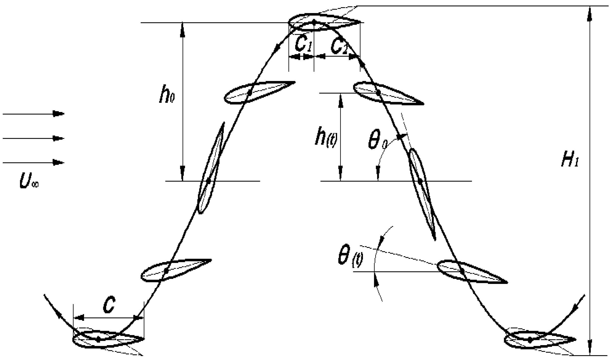
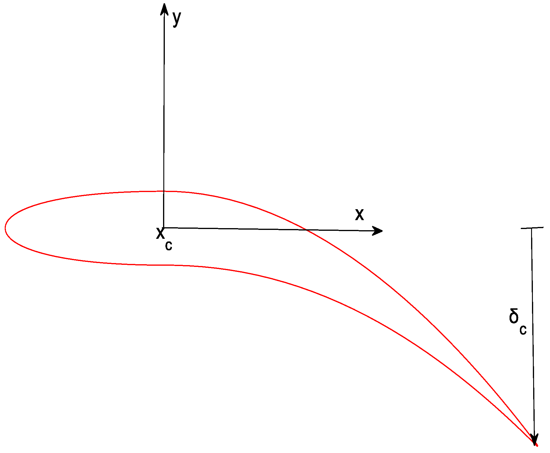
2. Hydrofoil Motion and Deformation Equation

In order to achieve the cyclical process of energy extraction in the flow field, the oscillating motion of the hydrofoil should be optimized as a coupled motion of heave and pitch. The heave motion refers to the translational motion of the hydrofoil, while the pitch motion refers to the rotation of the hydrofoil along the pitching axis. For the motion-constrained oscillating hydrofoil, the heave and pitch motion is designed as sinusoidal motion with the same frequency, which can be given as follows:

$$h(t)=h_0\sin (2\pi ft+\phi ),$$

(1)

$$\theta (t)={\theta }_0\sin (2\pi ft),$$

(2)

where, h(t) is the heave motion of the hydrofoil in the translational direction, which dominates the energy extraction from the tidal current, $\theta \left(t\right)$ is the pitch motion of the hydrofoil, which is the angle between the hydrofoil chord-wise and the incoming flow, h₀ and θ₀ are the amplitude of the oscillating hydrofoil heave and pitch motion separately, f is the oscillating frequency, φ is the phase angle difference between the heave and pitch motion, and φ is set here as 90°.

Figure 1 shows the kinetic model of the oscillating hydrofoil. The heaving velocity V_h(t) and the pitching angular velocity γ(t) of the oscillating hydrofoil obtained by the derivate Equations (1) and (2) are expressed as:

$$V_h(t)=2\pi f{h}_0\cos (2\pi ft+\phi ),$$

(3)

$$\gamma (t)=2\pi f{\theta }_0\cos (2\pi ft).$$

(4)

For the oscillating hydrofoil, two dimensionless parameters are defined. They are reduced frequency f* and Reynolds number Re:

$$f^{*}=\frac{fc}{U_{\infty }},$$

(5)

$$Re=\frac{U_{\infty }c}{\nu }.$$

(6)

Normally, there are three kinds of deformation for the hydrofoil. That is, (1) the leading-edge deformation, (2) the trailing edge deformation, and (3) the overall deformation. For simplicity, the leading-edge of the hydrofoil is set as rigid, and the trailing edge is set as flexible. Research on the chord-wise flexure of the hydrofoil was first applied to the bionic propulsion, and the propulsion performance was improved by optimizing the chord-wise flexure of the hydrofoil. Bose adopted the flexible trailing edge of the hydrofoil to improve the propulsion efficiency [22]. The chord-wise deformable equation is as follows:

$$y=8\delta {\left(x-0.5\right)}^3\cos \left(\omega t+\phi \right),x\ge 1/2.$$

(7)

Bionic propulsion and energy extraction are two forms for hydrofoil using energy in the flow field. Since they are similar in principle, Bose’s research results can be applied to the study of the oscillating hydrofoil energy extraction. After the modification, the hydrofoil chord deformable equation is formulated as:

$$y={\delta }_c\frac{x^n}{{\left(c-x_c\right)}^n}\sin \left(2\pi ft\right),$$

(8)

where, x_c is the starting point of hydrofoil deformation. Since the hydrofoil starts to deform from the pitching axis, and the pitching axis is located at c/3 from the leading-edge of the hydrofoil, the final deformable equation is as follows:

$$y={\delta }_c\frac{x^n}{{\left(2c/3\right)}^n}\sin \left(2\pi ft\right),0\le x\le \frac{2c}{3},$$

(9)

where, ${\delta }_c$ is the maximum chord offset at the trailing edge of the flexible hydrofoil, f is the frequency of the deformable motion, which is equal to the hydrofoil oscillation frequency, c is the hydrofoil chord length, and n is the flexibility coefficient of the hydrofoil. When the hydrofoil is rigid, the flexibility coefficient is n = 1 and the trailing edge offset is ${\delta }_c=0$. A larger n indicates a softer hydrofoil. The values of the flexibility coefficient are set as 1, 2, 5, and 10, and the maximum offsets at the trailing edge are 0, 0.05c, 0.1c, and 0.15c. Figure 2 shows the trailing edge deformation of the oscillating hydrofoil.

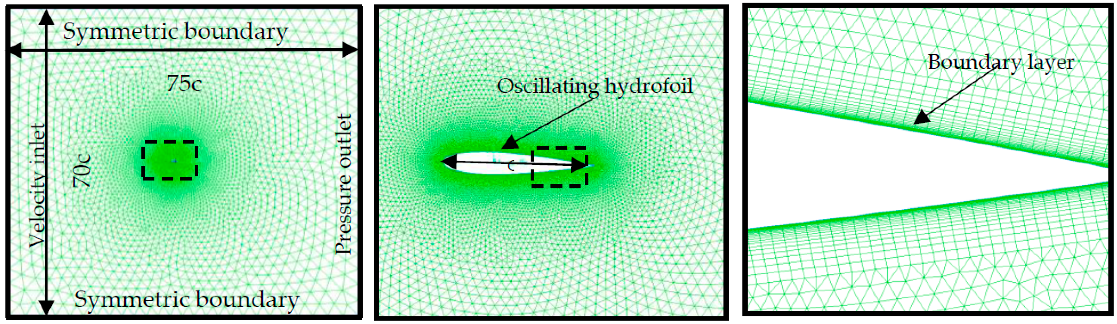
3. Numerical Calculation Method

The research on the effect of flexible hydrofoil on energy extraction, focuses on the chord-wise deformation in this paper. It does not involve the effect of span-wise deformation. Therefore, two-dimensional (2D) hydrofoil is regarded as the research object in this paper. The pre-processing software Gambit is used to mesh the flow field area, and the hydrofoil simulation model is established. Due to the large amplitude range of the hydrofoil movement, the surrounding mesh could be seriously distorted, and even the mesh reorganization could fail, which ultimately affects the accuracy of the simulation.

Therefore, the virtual surface method is used to encrypt the area near the hydrofoil in this paper, which improves the quality of the mesh in the process of motion.

In the turbulent flow field, the viscous effect appears on the surface of the hydrofoil and this is the boundary layer. The quality of the boundary layer meshing directly affects the correctness of the simulation results. During the numerical simulation process, the boundary layer meshing is divided by structure mesh. In this paper, 500 nodes are placed along the hydrofoil and are clustered close to the leading and trailing edges. The boundary conditions and an overview of mesh details are shown in Figure 3.

The commercial finite-volume computational fluid dynamics code FLUENT is used to perform the 2D simulation of hydrofoil. The Spalart-Allmaras turbulence model is adopted for the simulation, and the Pressure Implicit with Splitting of Operators (PISO) algorithm is selected for pressure and velocity coupling. The second-order schemes are used for pressure, momentum and turbulent viscosity resolution. In the simulation, the turbulence settings are a modified turbulent viscosity of 0.001 at the inlet and the oncoming flow velocity U_∞ is set to 1.8 m/s. Besides, user-defined functions (UDFs) are used to control the motion of the hydrofoil.

The motion and shape parameters of the hydrofoil are shown in

Table 1. Simulation parameters.

Hydrofoil	${\mathit{\chi }}_{\mathit{p}}$	$\mathit{\nu }\hspace{0.17em}{(\mathbf{m}}^2/\mathbf{s})$	$\mathit{\varphi }\hspace{0.17em}(\mathbf{rad})$	c (m)	${\mathit{U}}_{\mathit{\infty }}\hspace{0.17em}(\mathbf{m}/\mathbf{s})$	${\mathit{h}}_0$	Re	θo	n	δc
NACA0015	c/3	10−6	0.5π	0.22	1.8	c	500,000	720	1, 2, 5, 10	0, 0.05c, 0.1c, 0.15c

.

4. Energy Extraction Parameter

To extract energy from the oncoming flow, the hydrofoil motion is considered to be combined with heave and pitch motion. The instantaneous energy extraction power is defined as:

$$P\left(t\right)=P_y\left(t\right)+P_{\theta }\left(t\right)=F_y\left(t\right)V_h\left(t\right)+M\left(t\right)\gamma \left(t\right),$$

(10)

where, P_y(t) and P_θ(t) denote the energy extraction power from the heave motion and pitch motion respectively, while the F_y(t) and M(t) represent the force component in heave direction and the moment about the pitch axis. The average power during an oscillating cycle is as follows:

$$\stackrel{-}{P}=\frac{1}{T}\underset{t}{\overset{t+T}{{\displaystyle \int }}}P\left(t\right)dt,$$

(11)

where, T is the oscillating period. Therefore, the instantaneous power coefficient is expressed as:

$$C_P\left(t\right)=\frac{P\left(t\right)}{0.5\rho U_{\infty }{}^{3}c}=\frac{1}{U_{\infty }}\left(C_l(t)V_h\left(t\right)+c{C}_m(t)\gamma \left(t\right)\right),$$

(12)

where, ρ is the water density, and C_l(t) and C_m(t) are the instantaneous lift coefficient and momentum coefficient, respectively. They are defined as:

$$C_l\left(t\right)=\frac{F_y\left(t\right)}{0.5\rho U_{\infty }^{2}c},$$

(13)

$$C_m\left(t\right)=\frac{M\left(t\right)}{0.5\rho U_{\infty }^2{c}^2}.$$

(14)

After integration and averaging, the average power coefficient is defined as:

$$\stackrel{-}{C_P}=\frac{1}{T}\underset{t}{\overset{t+T}{{\displaystyle \int }}}{C}_P\left(t\right)dt.$$

(15)

In the uniform flow field, the total energy extraction from the flow is defined as:

$$P_a=0.5\rho U_{\infty }{}^3{H}_1,$$

(16)

where, H₁ is the overall vertical extent of the hydrofoil motion, as seen in Figure 1.

The definition of the hydrofoil energy extraction efficiency is expressed as:

$$\eta =\frac{\stackrel{-}{P}}{P_a}=\stackrel{-}{C_P}\frac{c}{A},$$

(17)

where, A is the swept area of the hydrofoil. The swept area A is equivalent to the swept height H₁ for the two-dimensional simulation of the oscillating hydrofoil.

5. Validation of the Numerical Results

In order to study the influence of the chord-wise flexibility on the energy extraction performance, this paper needs to verify the correctness of the simulation model. In the research field of oscillating hydrofoil energy extraction technology, researchers mostly verify the correctness of the model by comparing it with the simulation results from Reference [8]. In this paper, the correctness of the simulation model is also compared with the simulation results from Reference [8]. Parameter settings are consistent with those in Reference [8], which are shown in

Table 2. Simulation parameter settings for validating the model.

Hydrofoil	${\mathit{\chi }}_{\mathit{p}}$	$\mathit{\nu }\hspace{0.17em}{(\mathbf{m}}^2/\mathbf{s})$	$\mathit{\varphi }\hspace{0.17em}(\mathbf{rad})$	c (m)	${\mathit{U}}_{\mathit{\infty }}\hspace{0.17em}(\mathbf{m}/\mathbf{s})$	f*	${\mathit{h}}_0$	Re	θo
NACA0015	c/3	10−6	0.5π	0.25	2.0	0.14	c	500,000	750

.

In order to verify the correctness of the leading-edge vortex, the vorticity fields around the hydrofoil are compared with Reference [8]. As shown in Figure 4, the first row is the results of the model used in this paper and the second row is the results of Reference [8]. It can be seen that the size and the position of the vortex are basically the same as those from Reference [8]. At t/T = 0, the boundary layer is well separated. The vortex shedding and its moving tendency at t/T = 0.125, 0.25 also have a good consistency. Through the comparison of the vorticity fields, it is proven that the analysis of the vortex field is correct in this paper.

Figure 5 shows the comparison of the lift, torque and power coefficients in the same cycle of the hydrofoil with the same parameters. The solid red line is the simulation results in this paper, and the solid black line is the results from Reference [8]. As can be seen, the tendency of the curves is roughly the same, and the position of the fluctuations and curve peak are also very close. Due to the influence of meshing and boundary layer parameters’ selection, some gaps are generated, but the impact is not significant. These all indicate that the simulation results are correct in this paper.

6. Results and Discussion

This section mainly studies the effects of hydrofoil chord-wise deformation on hydrofoil attachment leading-edge vortex, hydrofoil surface pressure distribution, and lift force, so as to find how they affect the energy extraction performance. The feasibility of changing the chord-wise flexure of the oscillating hydrofoil to improve the hydrofoil energy extraction performance is also verified.

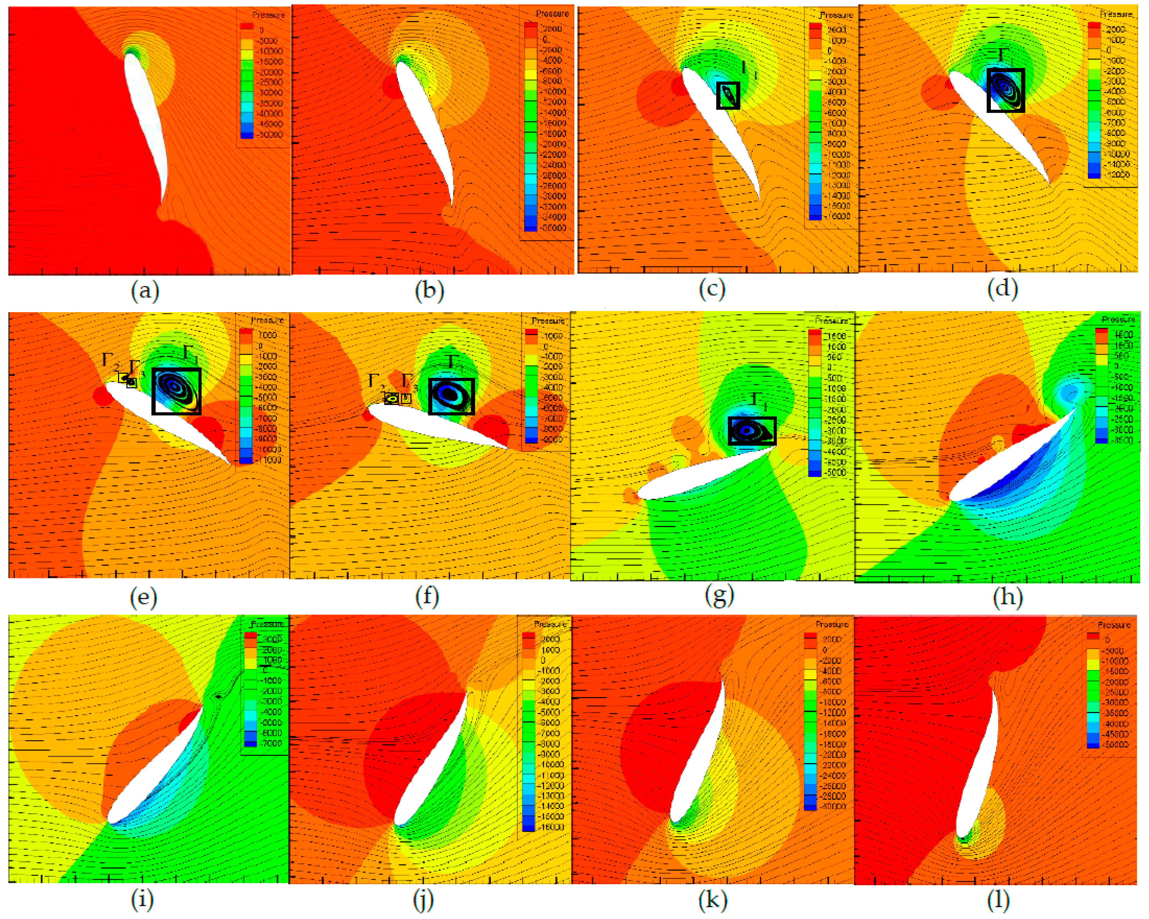
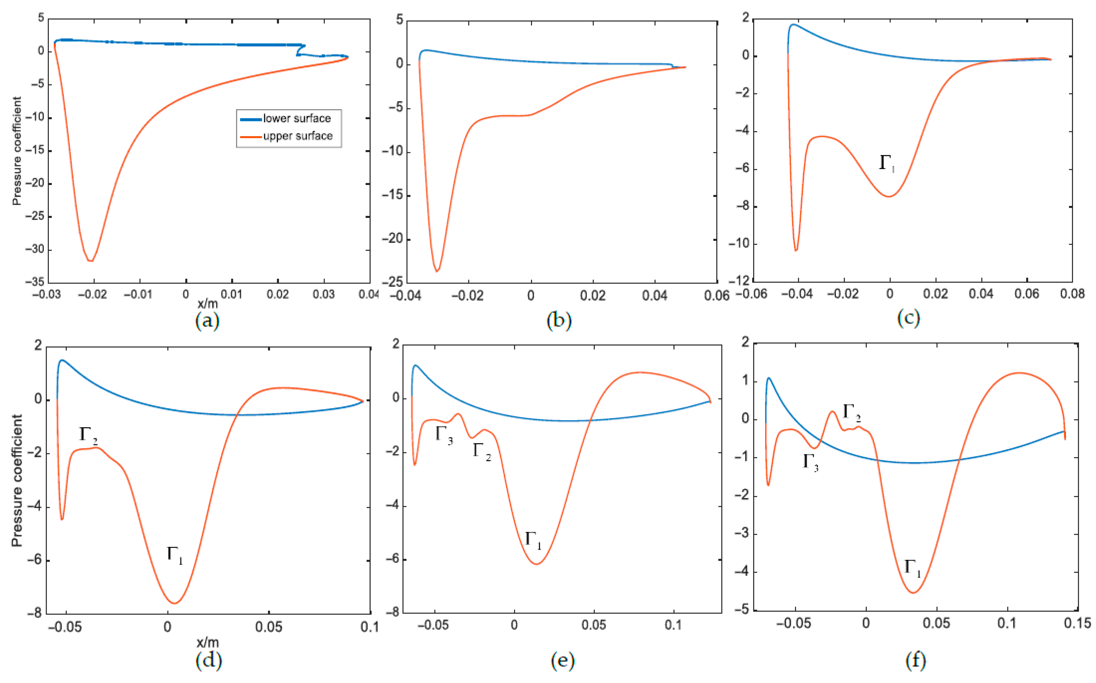
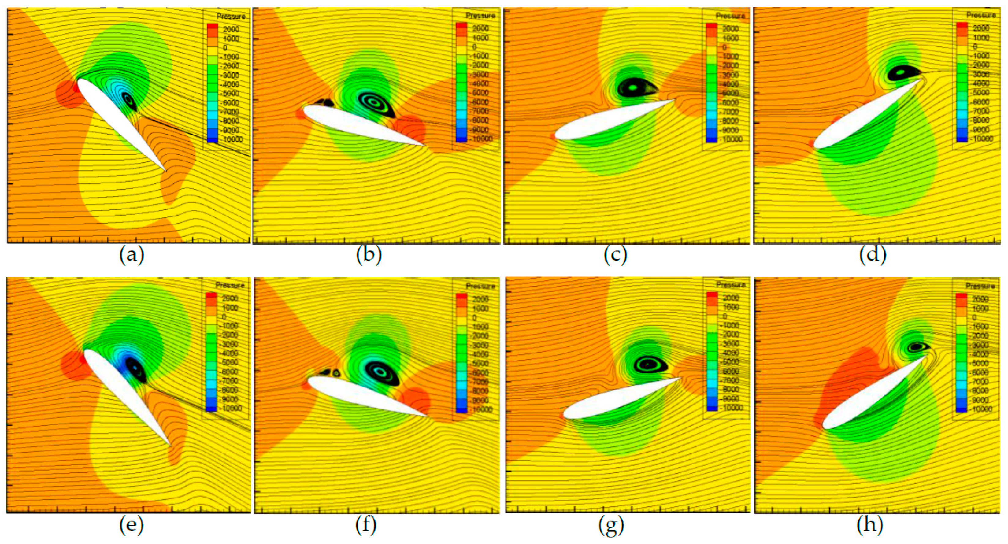
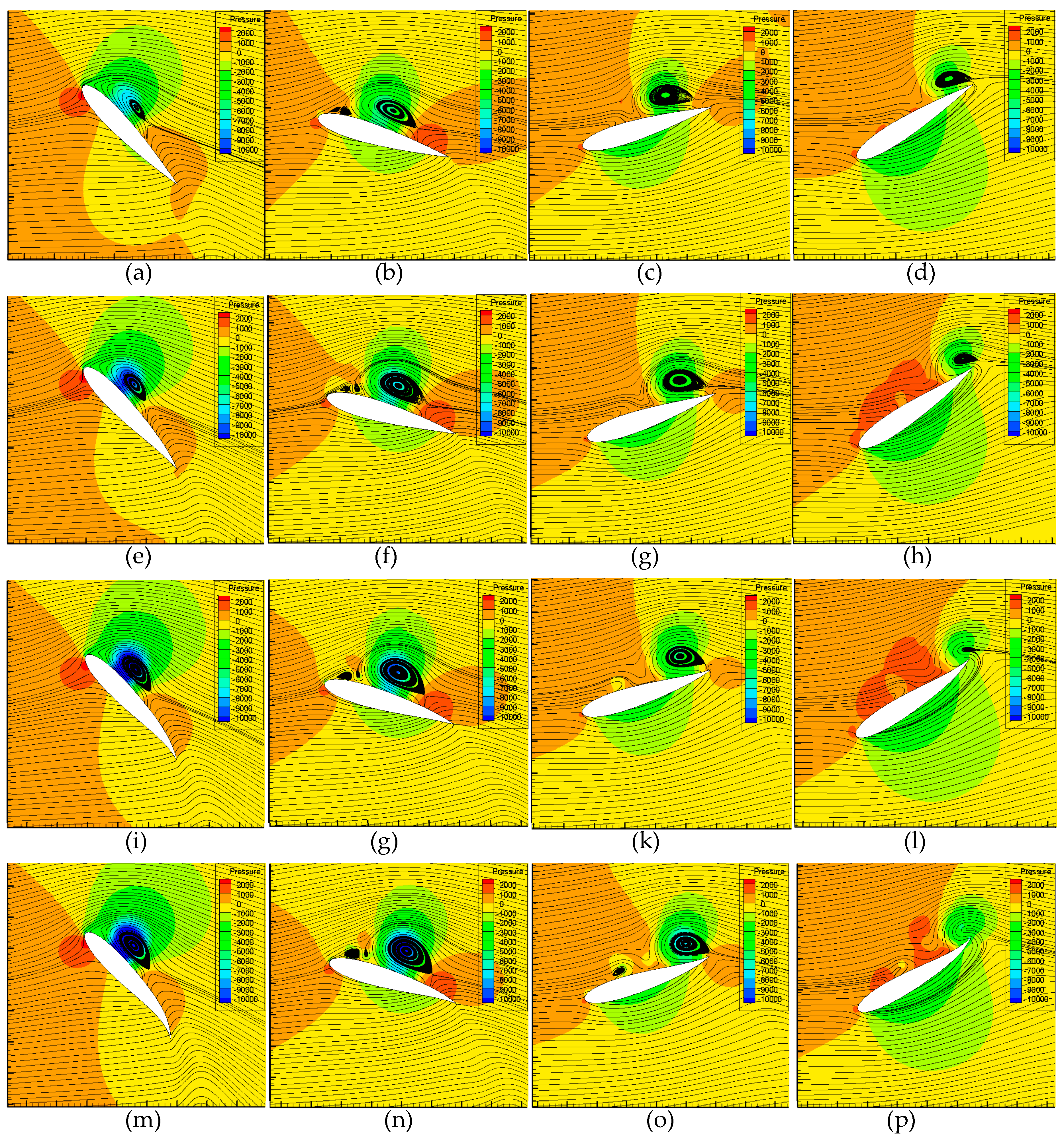
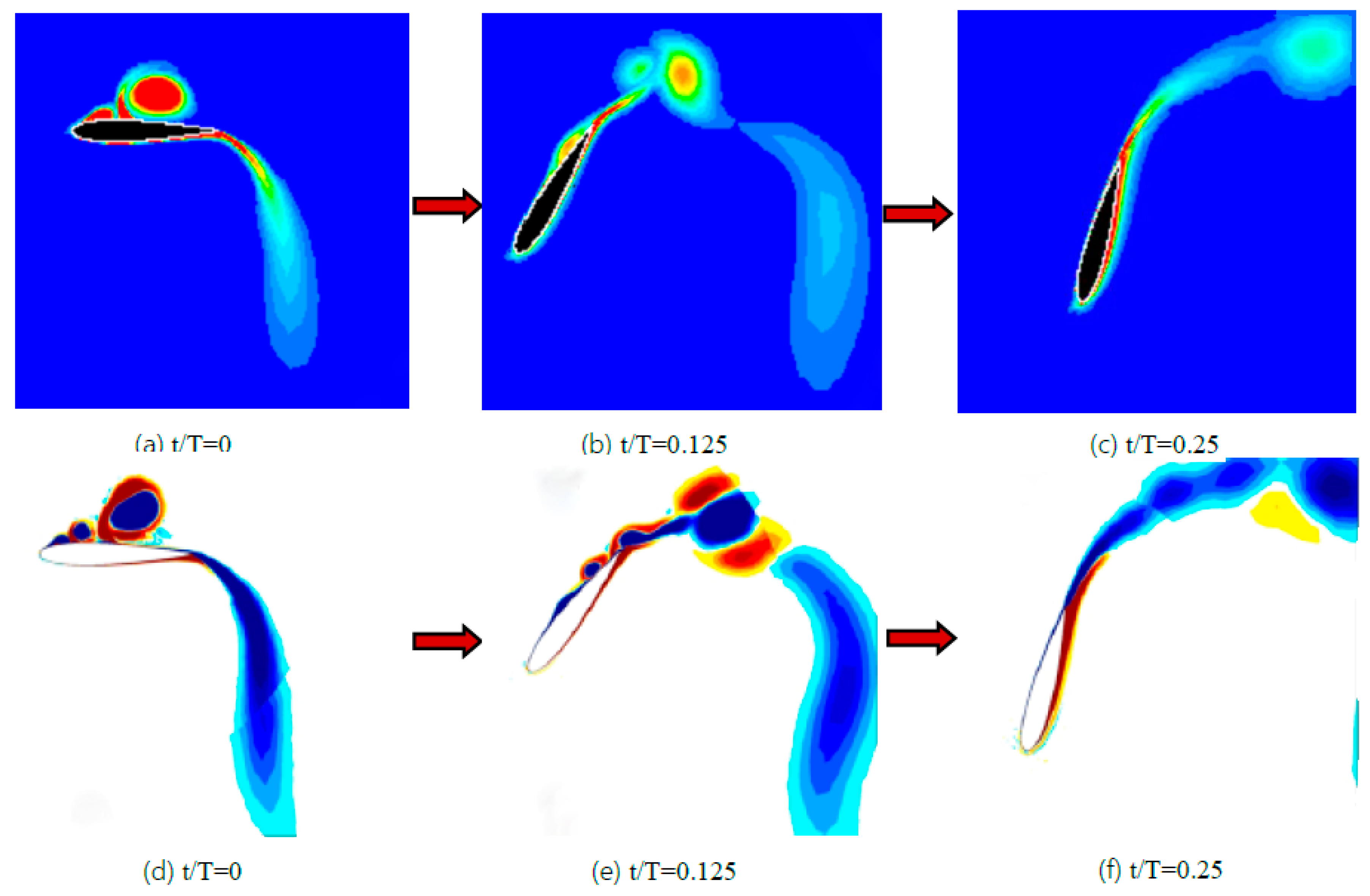
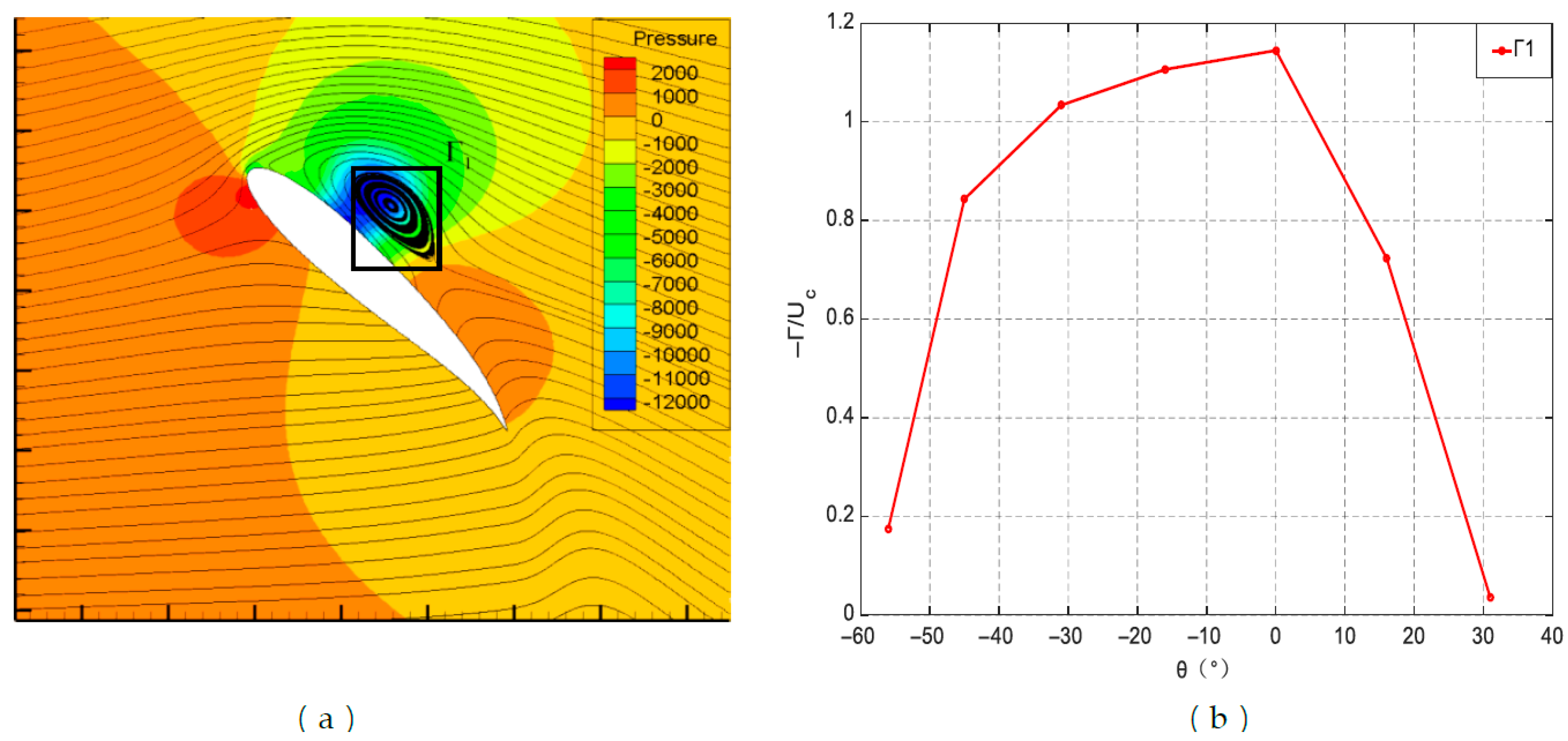
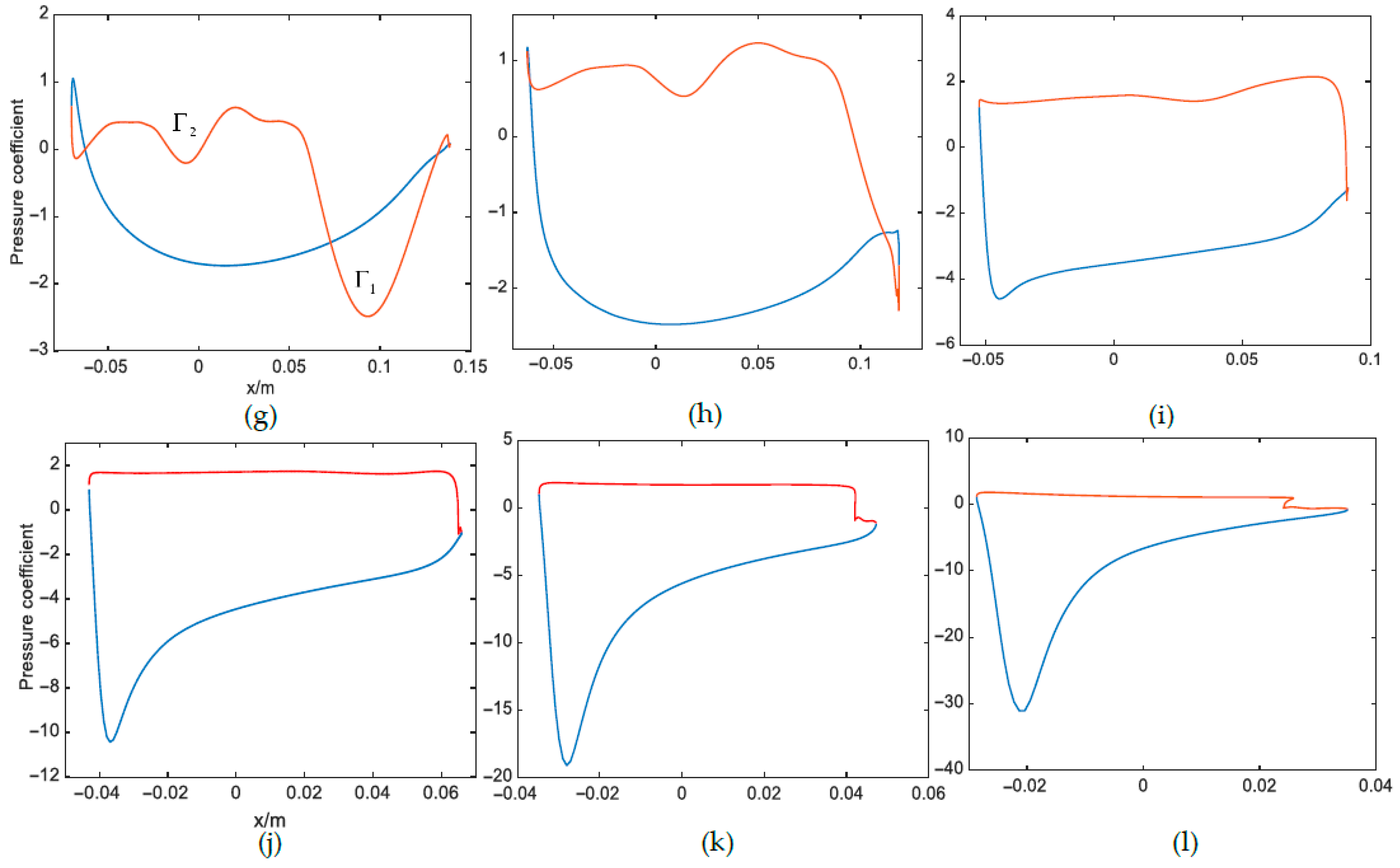
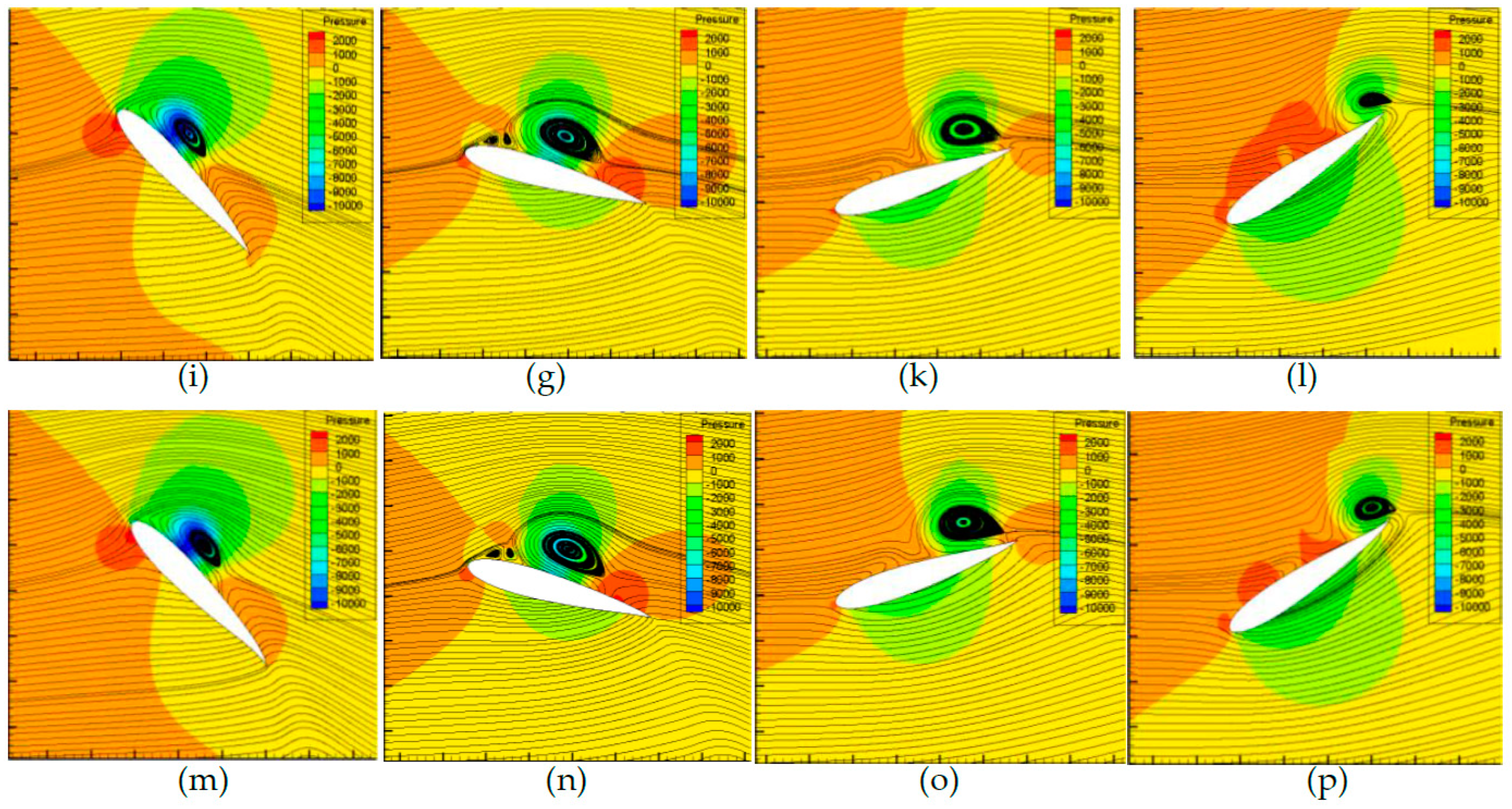
6.1. Quantification of the Attached Vortex and Its Relationship with Hydrofoil Pressure Distribution

According to the Kutta–Joukowsky theory, in inviscid flow, the lift force that acts on the hydrofoil is directly proportional to the vortex circulation, and the relationship is expressed in Equation (18), where F_L is the lift force on the hydrofoil, $\rho$ is the fluid density, U is the fluid velocity, and $\Gamma$ is the vortex circulation.

$$F_L=\rho U\Gamma .$$

(18)

In this paper, we studied the effect of the hydrofoil-attached vortex on the hydrodynamic performance of the hydrofoil with Equation (18). Due to the proportional relationship between the lift force on the hydrofoil and the vortex circulation, the strength of the vortex is expressed by the vortex circulation. In order to study the vortex behavior, we used circulation to examine the strength of vortices. The circulation near the attached vortex is calculated by the Stokes’ theorem. The Stokes’ theorem states that the velocity loop along the boundary line of an arbitrary, open curved surface is equal to the vortex flux through the curved surface. To sum up, the velocity loop amount also represents the amount of the vortex intensity. The specific expression is given as:

$$\Gamma ={\displaystyle \underset{A}{\oint }\upsilon }\cdot dl,$$

(19)

where, A is the closed curve in the velocity field, v is the velocity vector along the closed curve A, and the vortex circulation is obtained with integration.

In order to verify the relationship between the hydrofoil attachment vortex and the lift force, numerical simulations are performed with the parameters shown in Table 1. The chord-wise flexibility coefficient is 5, the maximum offset of the trailing edge is 0.1c, and the reduced frequency is 0.13.

Since the oscillating motion of the hydrofoil is cyclically reciprocating, the forming and shedding of the vortices from the hydrofoil is twice in one period. Because the two processes are repeated, a half-cycle is selected for comparison. Figure 6a is the streamline and pressure contour diagram of the vortex when the hydrofoil is at the pitch angle of −45°, and it depicts rectangular windows representing A for vortex core. The rectangular windows are adjusted to capture vortex circulation. Figure 6b shows the dimensionless −Γ/Uc as a function of the hydrofoil pitch angle during the half-cycle of the hydrofoil attachment vortex Γ1 from the forming and shedding.

Figure 7 illustrates the contours of the pressure coefficient with streamlines superimposed to represent the pressure distribution around the hydrofoil when the pitch angle θ is −72°, −65°, −56°, −45°, −31°, −16°, 16°, 31°, 45°, 56°, 65° and 72°, respectively. The forming and shedding process of the vortex from the hydrofoil surface during the half-cycle is shown. It can be seen from Figure 7 that the vortices are different in size and position during the process of formation and shedding, which is also the way to determine the different attachment vortex. From Figure 7, it can be found that the order of vortex formation is captured well, and each vortex core has only one peak during its lifetime. The maximum strength of Γ2 and Γ3 are lower than that of Γ1, and they appear and disappear quickly during the oscillating period. In summary, the leading-edge vortex Γ1 plays the most important role in the lift force generation for the hydrofoil. Therefore, the study on the influence of the hydrofoil attachment vortex on the hydrodynamic performance of the hydrofoil is mainly based on Γ1.

Figure 8 is the distribution of the pressure coefficient along the hydrofoil surface corresponding to Figure 7. Since the viscous action of the viscous fluid consumes the kinetic energy of the fluid, the surface of the hydrofoil forms a boundary layer when the hydrofoil oscillates in the flow field. The velocity is different when the fluid flows along the upper and lower surface of the hydrofoil, which causes a pressure difference between the two surfaces. Figure 7a and Figure 8 show that the pressure of the lower surface (red high-pressure region) and the upper surface (yellow and blue low-pressure regions) is different. It can be seen from the streamline that no fluid moves along the upper surface, and fluid backflow occurs in the boundary layer region. This causes the boundary layer to break away, and the expression is that the hydrofoil attachment vortex begins to form. The hydrofoil attachment vortex begins to form, as shown in Figure 7c,d. On the hydrofoil pressure curve, a local low pressure is generated at the position where the vortex is formed, as shown in Figure 8c,d. When the hydrofoil oscillates, the leading-edge vortex Γ1 begins to grow and move and the leading-edge vortex Γ2 and Γ3 appear, as shown in Figure 7e,f. As seen in Figure 8e,f, two small local low-pressures appear on the hydrofoil surface. This indicates that the vortex and low-pressure region have a one-to-one correspondence. As the vortex increases, the low-pressure region also increases. The most important factor affecting the pressure distribution on the hydrofoil surface is the leading-edge vortex. As the hydrofoil oscillates continuously, the leading-edge vortex also begins to move to the tail of the hydrofoil and gradually shed, as shown in Figure 7g–i. In Figure 8, the local low pressure on the surface gradually shifts back and disappears. Finally, as shown in Figure 8j–l, the lower surface and upper surface begin to perform the next boundary layer separation process.

In summary, Figure 7 shows the formation, movement and shedding of the hydrofoil leading-edge vortex. Figure 8 illustrates the pressure coefficient distribution over the hydrofoil surface at different pitch angles in the half-cycle. The following conclusions can be obtained by comparing Figure 7 with Figure 8: (1) The distribution of the pressure coefficient shows the one-to-one correspondence between the hydrofoil pressure coefficient and the hydrofoil leading-edge vortex. (2) The hydrofoil attachment vortex Γ1 has great influence on the hydrofoil surface pressure coefficient, whereas the influence of other attachment vortices can be neglected. Since the hydrofoil attachment vortex and the hydrofoil surface pressure coefficient distribution are in one-to-one correspondence, the relationship between the vortex circulation and the hydrofoil lift force is determined by Equations (18) and (19). By using the dimensionless value −Γ/Uc to define the vortex intensity, this paper combines with the relationship between lift and hydrofoil energy extraction performance to establish the relationship between the hydrofoil attachment vortex and the hydrodynamic performance of hydrofoil. Therefore, the influence of the hydrofoil chord-wise flexure on the hydrofoil is studied from the hydrofoil attachment vortex.

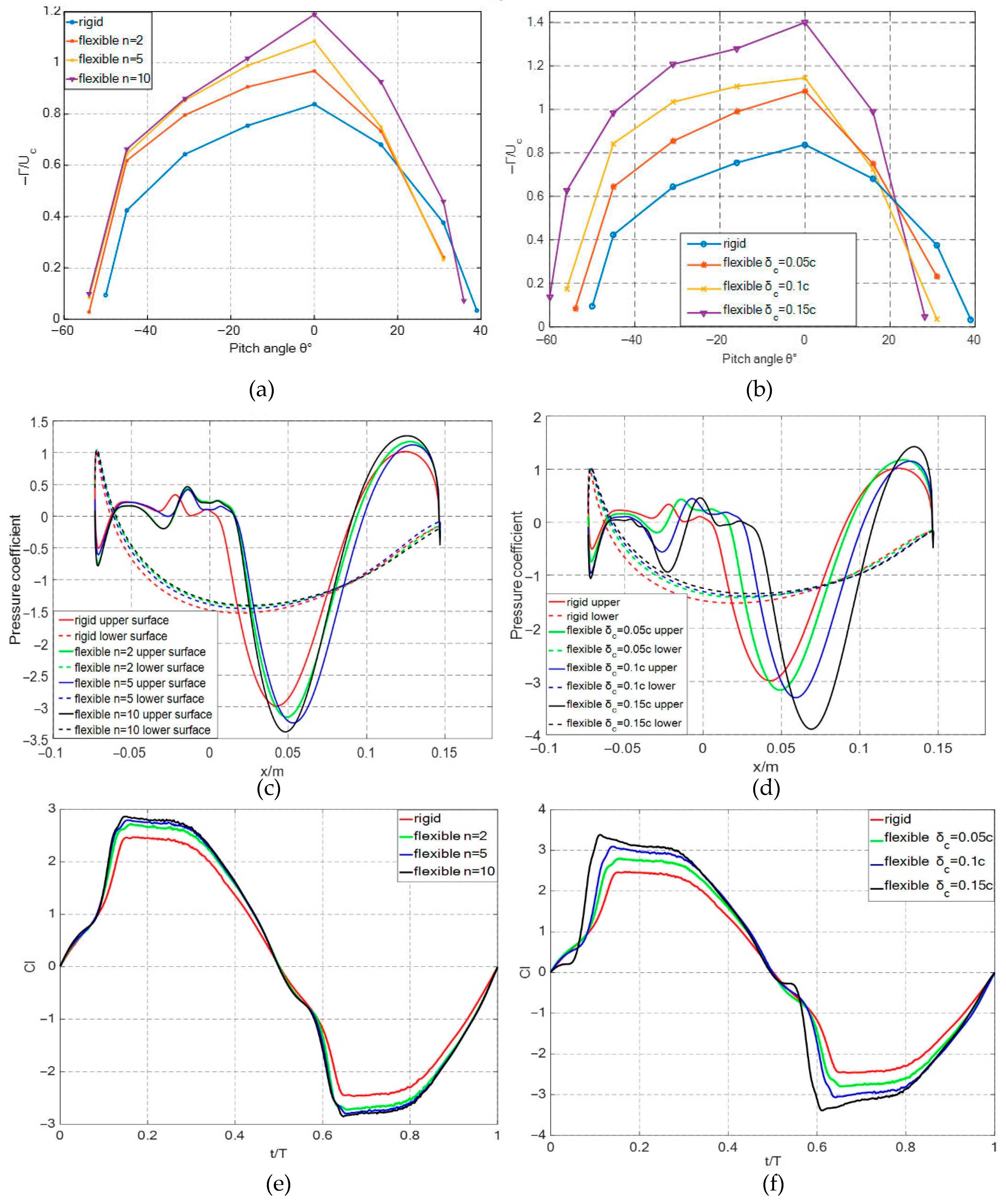
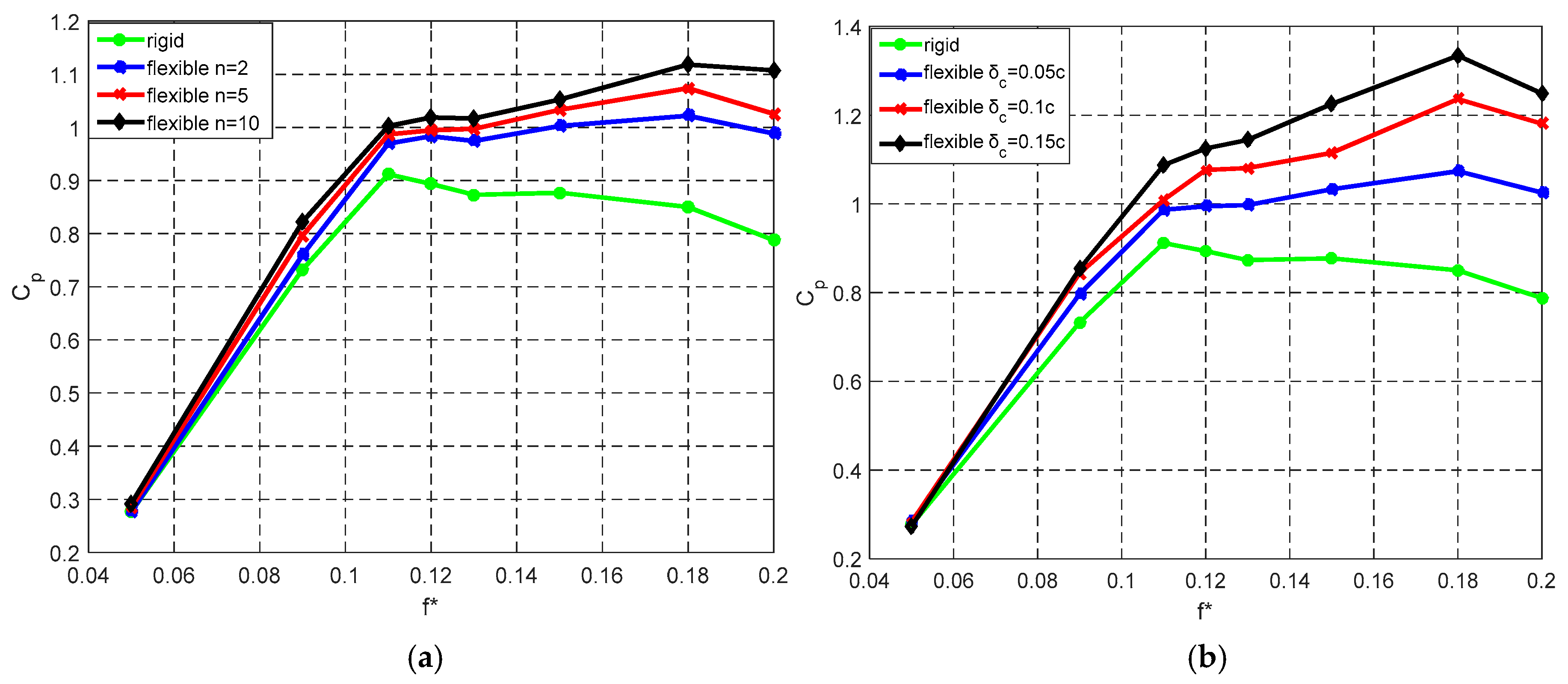
6.2. The Effect of Chord-Wise Flexure on Hydrofoil Lift

According to Figure 7 and Figure 8, the relationship between the hydrofoil attachment vortex and the lift is obtained. Therefore, it is necessary to study how the chord-wise flexure affects the lift from the vortex circulation analysis.

To further study the effects of chord-wise flexibility on the leading-edge vortex, contours and streamlines for comparing the effect of the flexibility coefficient (n) and the effect of the trailing edge offset (δc) on the leading-edge vortex were plotted.

Contours of vortices with different flexibility coefficients and different pitch angles (θ = −45°, −16°, 16°, 31°) are shown in Figure 9 in the case of δc = 0.05c. It can be seen from f that vortex intensity of the flexible hydrofoil is greater than that of the rigid hydrofoil when θ = −45° and θ = −16°. The vortex intensity seems to be stronger with the flexibility coefficient increasing. The vortex intensity is also stronger with the flexibility coefficient increasing when θ = 16° and θ = 31°, but not all of them are stronger than that of the rigid hydrofoil.

Contours of vortices with different trailing edge offsets and different pitch angles (θ = −45°, −16°, 16°, 31°) are shown in Figure 10 in the case of n = 5. The vortex intensity of the flexible hydrofoil is significantly enhanced with the trailing edge offset increasing when θ = −45° and θ = −16° and all of them are much greater than that of the rigid hydrofoil. The effect of the trailing edge offset on vertex intensity is irregular when θ = 16°. But the increasing of the trailing edge offset significantly reduces the strength of the vortices when θ = 31°. Even the leading-edge vortex from the hydrofoil surface has completely shed off at δc = 0.15c. It shows that the increasing of the trailing edge offset accelerates the shedding of the attached vortex.

Combined with Figure 9 and Figure 10, it is easy to find that the effect of the flexibility coefficient and the effect of the trailing edge offset on the attached vortex are similar and accelerate the vortex shedding. But the effect of the trailing edge offset on the vortex is greater. In order to better analyze the effect of the flexibility coefficient and the effect of the trailing edge offset on the hydrofoil surface-attached vortex. The vortex is quantified to analyze the effect of the chord-wise flexure on the energy extraction performance.

According to the Kutta−Joukowsky theory and the Stokes’ theorem, the vortex can be quantified by vortex circulation, and the intensity of the vortex can be expressed by the dimensionless value, i.e., −Γ/Uc. The quantified results consist of different angles (θ = −45°, −31°, −16°, 0°, 16°, 31°) and the forming and shedding positions of the vortex are shown in Figure 11a,b. Due to the relationship of vortex circulation and the lift of the hydrofoil, the effects of chord-wise flexure on hydrofoil lift can be obtained through the comparison of −Γ/Uc.

As seen from Figure 11a,b, −Γ/Uc shows a parabolic trend with the change of the pitch angle and reaches a peak when the pitch angle equals zero. As the flexibility coefficient increases, the leading-edge vortex of the hydrofoil is generated earlier and −Γ/Uc becomes larger. This means that increasing the flexibility coefficient causes the leading-edge vortex to appear earlier and fall off faster after the vortex reaches the peak. According to the study of the leading-edge vortex, the leading-edge vortex appears earlier, and the increasing of the vortex intensity increases the pressure coefficient difference of the hydrofoil surface. As expressed in Figure 11c,d, the hydrofoil surface pressure coefficient difference increases with the hydrofoil flexibility coefficient. As is shown in Figure 11e,f, the hydrofoil instantaneous lift coefficient increases with the flexibility coefficient. In summary, the chord-wise deformation can improve pressure distribution on the hydrofoil surface by increasing the intensity of the vortex, so as to enhance the lift coefficient that acts on the hydrofoil.

6.3. The Effect of Chord-Wise Flexure on Hydrofoil Energy Extraction

It was found from Equation (12) that the oscillating hydrofoil extracts energy through the process of heave motion and pitch motion. The lift coefficient that acts on the hydrofoil is enhanced by introducing the chord-wise flexure. Therefore, the total power that is extracted by the hydrofoil is increased.

Table 3. Average power coefficient of hydrofoil under different flexibility coefficients and trailing edge offsets.

Hydrofoil	Total Average Power Coefficient	Average Power Coefficient of the Heave Motion	Average Power Coefficient of the Pitch Motion
Rigid hydrofoil	0.8731	0.9744	−0.1013
Flexibility coefficient n = 2	0.9743	1.0947	−0.1204
Flexibility coefficient n = 5	0.9972	1.1304	−0.1332
Flexibility coefficient n = 10	1.0168	1.1547	−0.1379
Maximum offset ${\delta }_c$ = 0.05c	0.9972	1.1304	−0.1332
Maximum offset ${\delta }_c$ = 0.1c	1.0808	1.2345	−0.1537
Maximum offset ${\delta }_c$ = 0.15c	1.1441	1.3258	−0.1817

shows the total average power coefficient, heave motion and pitch motion average power coefficients respectively, when the reduced frequency f* is 0.13. It can be concluded that the total energy extraction power rises with the flexibility coefficient and the trailing edge offset. For the average power from heave motion and pitch motion, the energy extraction from heave motion increases with the flexibility coefficient and trailing edge offset, whereas the energy extraction from pitch motion decreases. But the contribution of the energy extraction from heave motion is greater than that form the pitch motion. So, we can conclude that the energy extraction increases with the flexibility coefficient and the trailing edge offset.

Figure 12 shows that the total average power coefficient of the oscillating hydrofoil changes with different flexibility coefficients and trailing edge offsets. It can be seen that the flexibility coefficient and the maximum offset have little effect on the energy extraction performance when the reduced frequency f* is smaller than 0.08. However, when f* is higher than 0.08, the energy extraction performance of the hydrofoil is greatly increased with the flexibility coefficient and the maximum offset. The maximum total average power coefficient is increased from 0.912 to 1.118 and 1.334, respectively.

7. Conclusions

In this paper, the energy extraction performance of the oscillating hydrofoil with chord-wise flexibility was analyzed by quantifying the vortex that is attached to the hydrofoil surface. By defining the vortex intensity with the dimensionless value −Γ/Uc, the relationship between the hydrofoil attachment vortex and energy extraction performance of the hydrofoil was established. By analyzing the contours of vortices with streamlines and the pressure distribution along the hydrofoil surfaces, we concluded that the evolution of the hydrofoil attachment vortex has a great effect on the pressure distribution along the hydrofoil surface. The largest attached vortex had the main effect on the pressure distribution, and other small attached vortices could be neglected.

The effect of the hydrofoil chord-wise flexure on the energy extraction performance was studied with the hydrofoil attachment vortex. We concluded that, by introducing the chord-wise flexure of the hydrofoil, the hydrofoil attachment vortex appears earlier and falls off faster, and this helps to enhance the intensity of the leading-edge vortex, as well as the lift force that acts on the hydrofoil. So, the hydrofoil energy extraction performance is enhanced by introducing the chord-wise flexibility.

This paper only carried out the numerical analysis, experiments should be done in the next step. However, it is reasonable to believe that the results of this paper could provide vital guidance for experiment design and industry application of oscillating hydrofoil energy extraction devices.

References

1. McKinney, W.; DeLaurier, J. Wingmill: An oscillating-wing windmill. J. Energy 1981, 5, 109–115. [Google Scholar] [CrossRef]
2. Platzer, M.; Ashraf, M.; Young, J. Development of a new oscillating-wing wind and hydropower generator. In 47th Aerospace Sciences Meeting; AIAA: Reston, VA, USA, 2013. [Google Scholar]
3. Ashraf, M.; Young, J.; Lai, J.C.S.; Platzer, M.F. Numerical analysis of an oscillating-wing wind and hydropower generator. AIAA J. 2011, 49, 1374–1386. [Google Scholar] [CrossRef]
4. Zhu, Q. Optimal frequency for flow energy harvesting of a flapping foil. J. Fluid Mech. 2011, 675, 495–517. [Google Scholar] [CrossRef]
5. Kinsey, T.; Dumas, G. Optimal operating parameters for an oscillating foil turbine at Reynolds number 500,000. AIAA J. 2014, 52, 1885–1895. [Google Scholar] [CrossRef]
6. Kinsey, T.; Dumas, G. Three-dimensional effects on an oscillating-foil hydrokinetic turbine. J. Fluids Eng. 2012, 134, 071105. [Google Scholar] [CrossRef]
7. Kinsey, T.; Dumas, G.; Lalande, G.; Ruel, J.; Mehut, A. Prototype testing of a hydrokinetic turbine based on oscillating hydrofoils. Renew. Energy 2011, 36, 1710–1718. [Google Scholar] [CrossRef]
8. Kinsey, T.; Dumas, G. Computational fluid dynamics analysis of a hydrokinetic turbine based on oscillating hydrofoils. J. Fluids Eng. 2012, 134, 021104. [Google Scholar] [CrossRef]
9. Xu, J.A.; Sun, H.Y.; Tan, S.L. Wake vortex interaction effects on energy extraction performance of tandem oscillating hydrofoils. J. Mech. Sci. Technol. 2016, 30, 4227–4237. [Google Scholar] [CrossRef]
10. Xu, J.A.; Tan, S.L.; Guan, D.T. Energy extraction performance of motion constrained tandem oscillating hydrofoils. J. Renew. Sustain. Energy 2017, 9, 044501. [Google Scholar] [CrossRef]
11. Lindsey, K. A Feasibility Study of Oscillating-Wing Power Generation; United States Naval Postgraduate School: Monterey, CA, USA, 2002. [Google Scholar]
12. Usoh, C.O.; Young, J.; Lai, J.C.S. Numerical analysis of a non-profiled plate for flapping wing turbines. In Proceedings of the 18th Australian Fluid Mechanics Conference, Launceston, Australia, 3–7 December 2012. [Google Scholar]
13. Wei, S.; Liu, H. Flapping wings and aerodynamic lift: The role of leading edge vortices. AIAA J. 2007, 45, 2817–2819. [Google Scholar]
14. Ellington, C.P.; van den Berg, C.; Willmott, A.P.; Thomas, A.L.R. Leading-edge vortices in insect flight. Nature 1996, 384, 626. [Google Scholar] [CrossRef]
15. Huang, B.; Wu, Q.; Wang, G.Y. Numerical simulation of unsteady cavitating flows around a transient pitching hydrofoil. Sci. China Technol. Sci. 2014, 57, 101–116. [Google Scholar] [CrossRef]
16. Kevin, D.J.; Lindsey, K.; Platzer, M.F. An investigation of the fluid-structure interaction in an oscillating-wing micro-hydropower generator. WIT Trans. Built Environ. 2003, 71, 10. [Google Scholar]
17. Kinsey, T.; Dumas, G. Parametric study of an oscillating airfoil in a power-extraction regime. AIAA J. 2008, 46, 1318–1330. [Google Scholar] [CrossRef]
18. Liu, W.D.; Xiao, Q.; Cheng, F. A bio-inspired study on tidal energy extraction with flexible flapping wings. Bioinspir. Biomim. 2013, 8, 1–11. [Google Scholar] [CrossRef]
19. Zhu, B.; Xia, P.; Huang, Y.; Zhang, W. Energy extraction properties of a flapping wing with an arc-deformable airfoil. J. Renew. Sustain. Energy 2019, 11, 023302. [Google Scholar] [CrossRef]
20. Hoke, C.M.; Young, J.; Lai, J.C.S. Effects of time-varying camber deformation on flapping foil propulsion and power extraction. J. Fluids Struct. 2015, 56, 152–176. [Google Scholar] [CrossRef]
21. Wu, Y.J.; Wu, J.; Tian, F.B. How a flexible tail improves the power extraction efficiency of a semi-activated flapping foil system: A numerical study. J. Fluids Struct. 2015, 54, 886–899. [Google Scholar] [CrossRef]
22. Bose, N. Performance of chord-wise flexible oscillating propulsors using a time-domain panel method. Int. Shipbuild. Prog. 1995, 42, 281–294. [Google Scholar]
Figure 1. Kinetic model of the oscillating hydrofoil.
Jmse 07 00398 g001
Figure 2. Trailing edge deformation model.
Jmse 07 00398 g002
Figure 3. Computational domain and mesh distribution.
Jmse 07 00398 g003
Figure 4. Comparison of the vorticity fields between the simulation model of this paper and Reference [8] at f* = 0.14. (ac) The vorticity fields of the simulation model in this paper. (df) The vorticity fields of Reference [8].
Jmse 07 00398 g004
Figure 5. Comparison of lift, momentum and power coefficient in the same cycle at f* = 0.14 (the solid red lines show simulation results with the Spalart-Allmaras (SA) model and the solid black lines show results from Reference [8]). (a) Lift coefficient. (b) Momentum coefficient. (c) Power coefficient.
Jmse 07 00398 g005
Figure 6. (a) Contours of vortices with streamlines and pressure of flexible hydrofoil (n = 5, δc = 0.1c, f* = 0.13) with θ = 45°. (b) The curve diagram of −Γ/Uc change with pitch angle in the case n = 5, δc = 0.1c and f* = 0.13.
Jmse 07 00398 g006
Figure 7. Contours of vortices with streamlines and pressure of flexible hydrofoil (n = 5, δc = 0.1c, f* = 0.13) in the half-cycle. (a) θ = −72°, (b) θ = −65°, (c) θ = −56°, (d) θ = −45°, (e) θ = −31°, (f) θ = −16°, (g) θ = 16°, (h) θ = 31°, (i) θ = 45°, (j) θ = 56°, (k) θ = 65°, (l) θ = 72°.
Jmse 07 00398 g007
Figure 8. Distribution of the pressure coefficient along the flexible hydrofoil surfaces (n = 5, δc = 0.1c, f* = 0.13) in the half-cycle. (a) θ = −72°, (b) θ = −65°, (c) θ = −56°, (d) θ = −45°, (e) θ = −31°, (f) θ = −16°, (g) θ = 16°, (h) θ = 31°, (i) θ = 45°, (j) θ = 56°, (k) θ = 65°, (l) θ = 72°.
Jmse 07 00398 g008aJmse 07 00398 g008b
Figure 9. Contours of vortices with streamlines and pressure (Pa) of flexible hydrofoil in the case δc = 0.05c and f* = 0.13 (the thicker the blue, the stronger the vortex). (a) rigid, θ = −45°, (b) rigid, θ = −16°, (c) rigid, θ = 16°, (d) rigid, θ = 31°, (e) n = 2, θ = −45°, (f) n = 2, θ = −16°, (g) n = 2, θ = 16°, (h) n = 2, θ = 31°, (i) n = 5, θ = −45°, (j) n = 5, θ = −16°, (k) n = 5, θ = 16°, (l) n = 5, θ = 31°, (m) n = 10, θ = −45°, (n) n = 10, θ = −16°, (o) n = 10, θ = 16°, (p) n = 10, θ = 31°.
Jmse 07 00398 g009aJmse 07 00398 g009b
Figure 10. Contours of vortices with streamlines and pressure (Pa) of flexible hydrofoil in the case n = 5 and f *= 0.13 (the thicker the blue, the stronger the vortex). (a) rigid, θ = −45°, (b) rigid, θ = −16°, (c) rigid, θ = 16°, (d) rigid, θ = 31°, (e) δc = 0.05c, θ = −45°, (f) δc = 0.05c, θ = −16°, (g) δc = 0.05c, θ = 16°, (h) δc = 0.05c, θ = 31°, (i) δc = 0.1c, θ = −45°, (j) δc = 0.1c, θ = −16°, (k) δc = 0.1c, θ = 16°, (l) δc = 0.1c, θ = 31°, (m) δc = 0.15c, θ = −45°, (n) δc = 0.15c, θ = −16°, (o) δc = 0.15c, θ = 16°, (p) δc = 0.15c, θ = 31°.
Jmse 07 00398 g010
Figure 11. (a,b) Comparison of Γ / U c with different pitch angles at f* = 0.13. (c,d) Comparison of the pressure coefficient of the hydrofoil surface with θ = 0 at f* = 0.13. (e,f) Comparison of lift coefficient with different chord-wise flexible hydrofoils at f* = 0.13. Here, (a,c,e) Fixed δc = 0.05c, (b,d,f) Fixed n = 5.
Jmse 07 00398 g011
Figure 12. Comparison of average power coefficient among different chord-wise flexible hydrofoil under different reduced frequencies. (a) Fixed δc = 0.05c. (b) Fixed n = 5.
Jmse 07 00398 g012