Analysis of Slope Failure Behaviour Based on Real-Time Measurement Using the x–MR Method

 ,
,
Abstract
1. Introduction
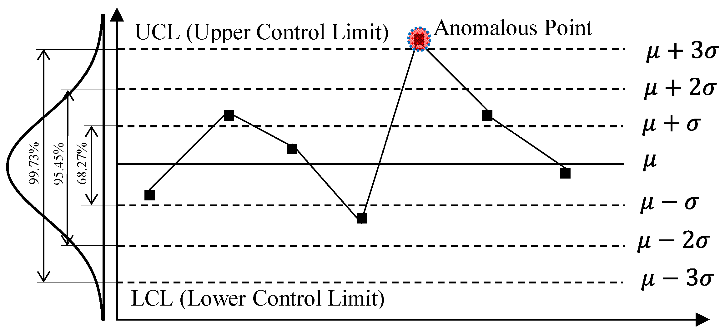
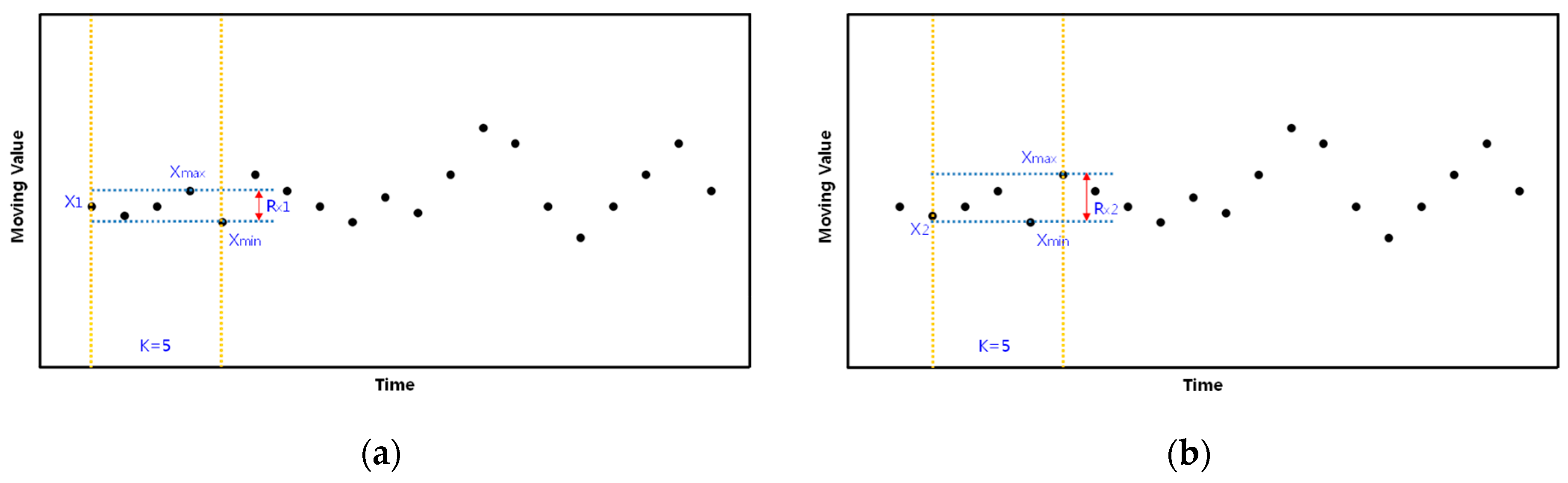
2. x–MR Control Chart
3. Real Scale Slope Failure Simulation
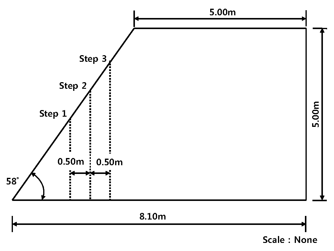
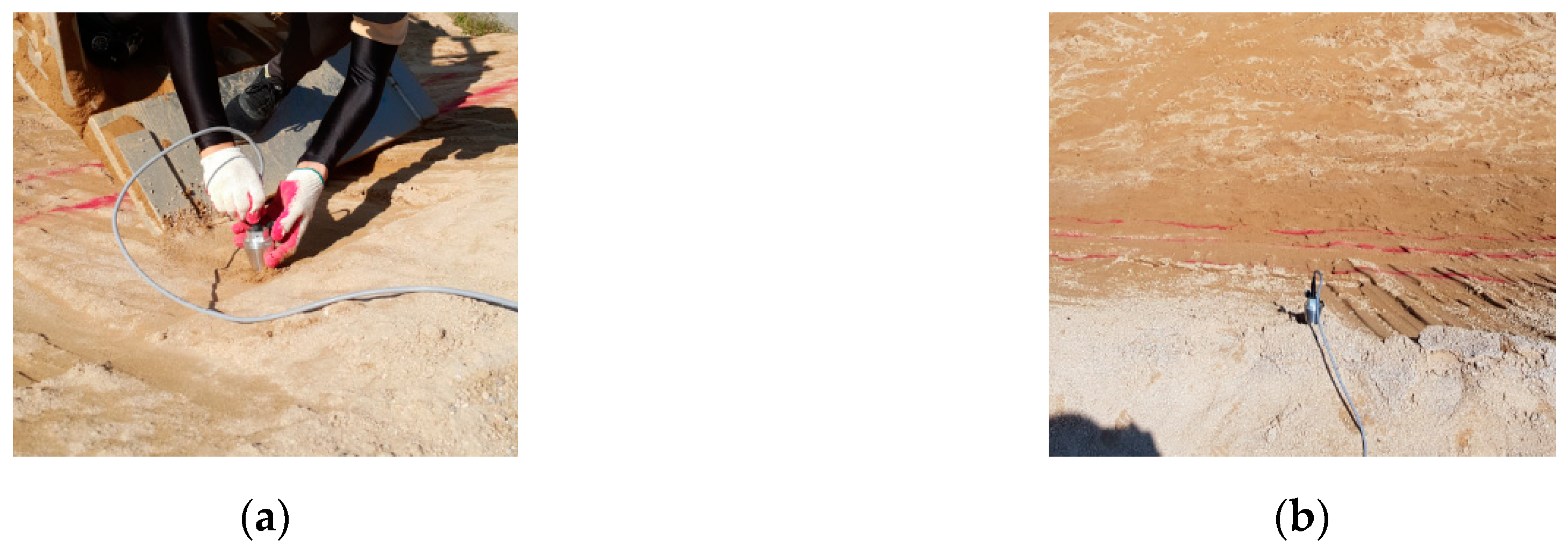
3.1. Real Scale Slope Construction for Slope Failure Simulation
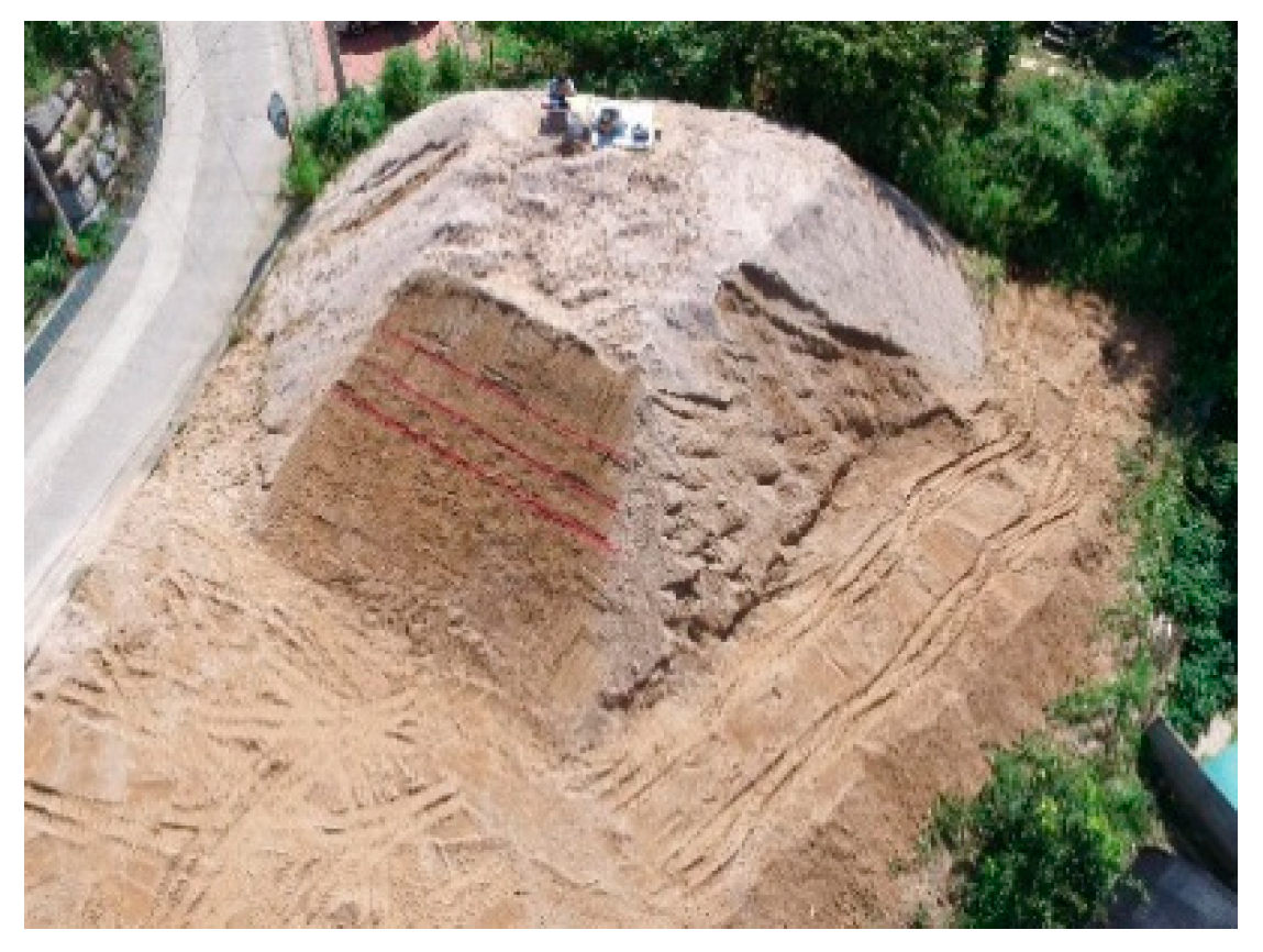
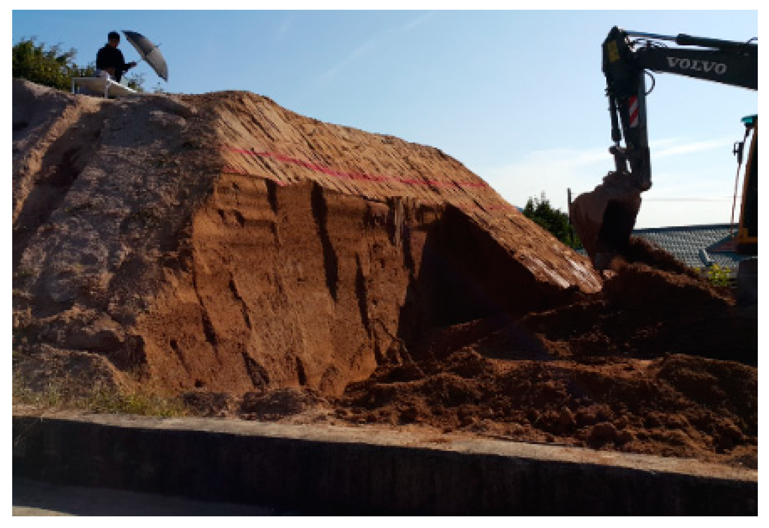
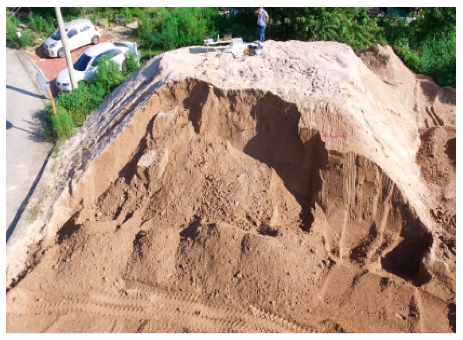
3.2. Slope Failure Simulation by Slope Cutting
4. Analysis of Experimental Results
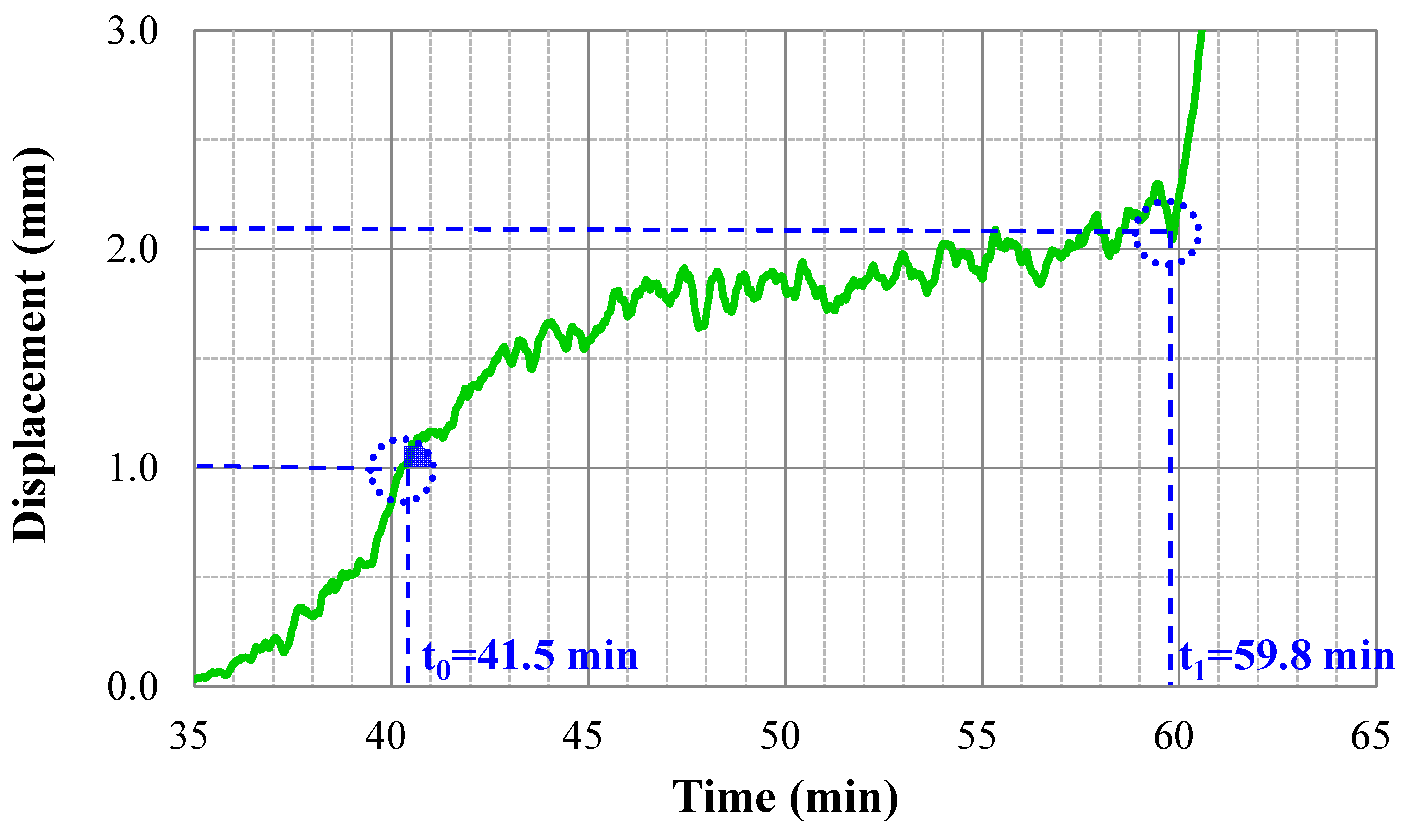
4.1. Analysis of the Behaviour of Slope Failure
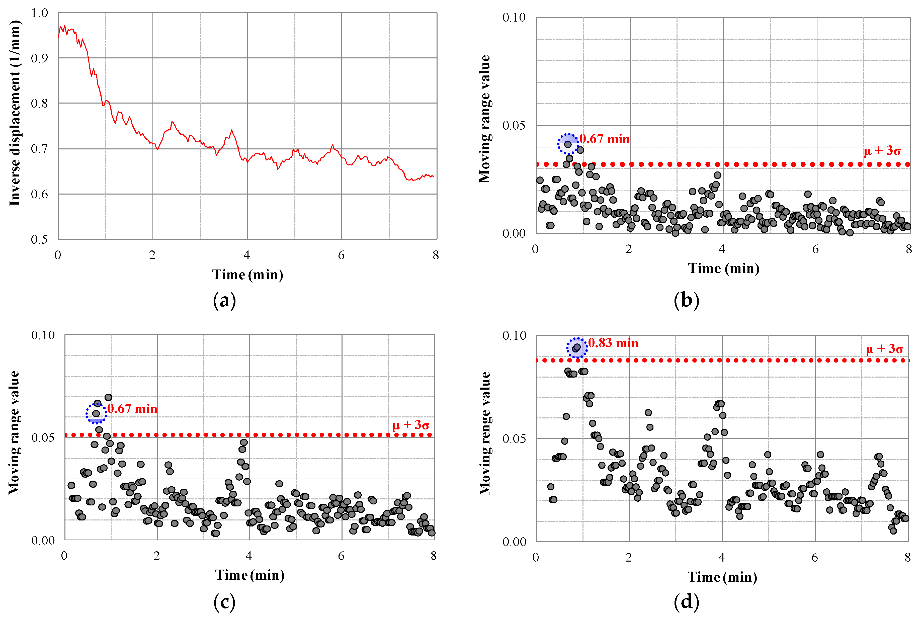
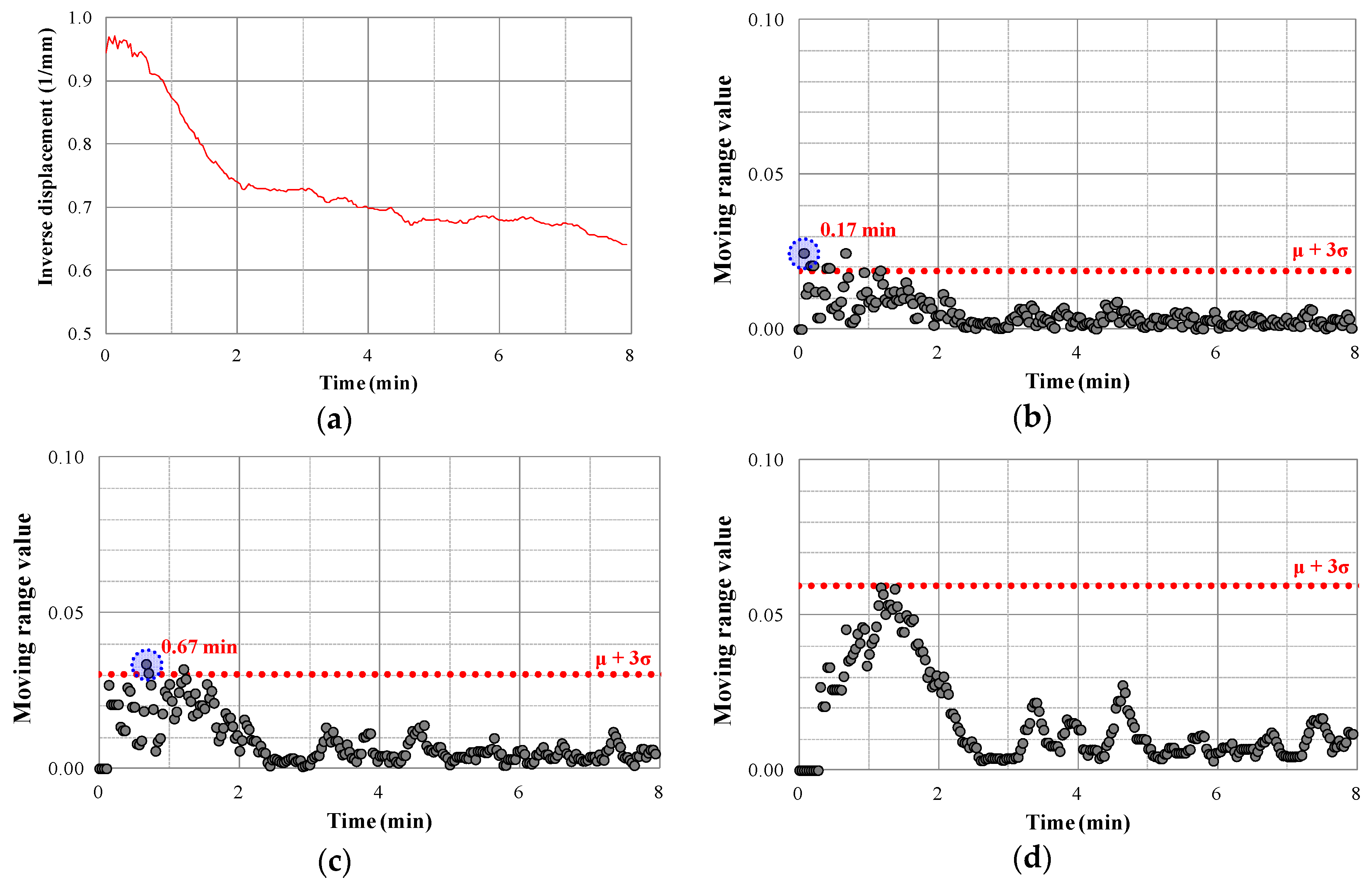
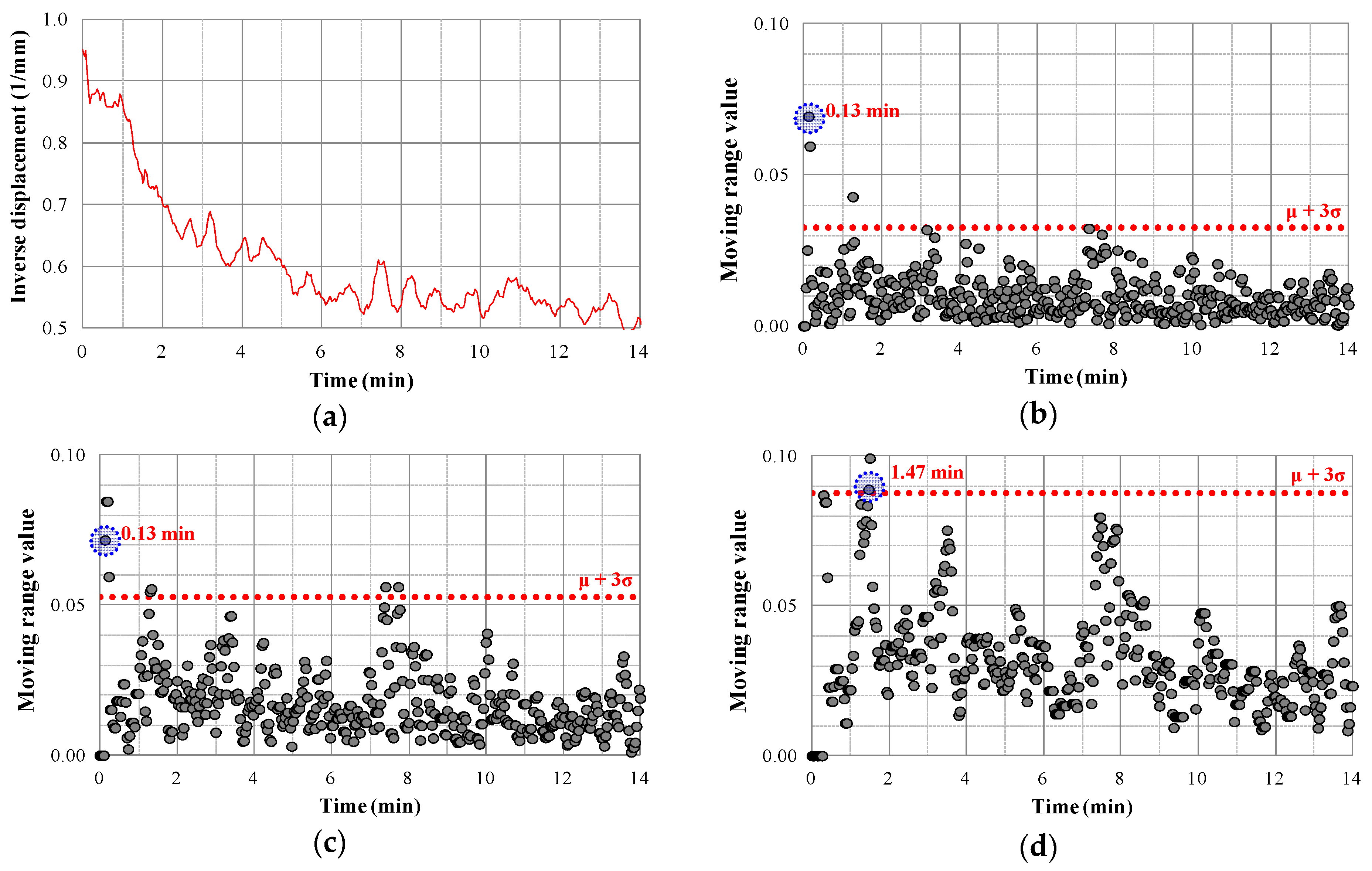
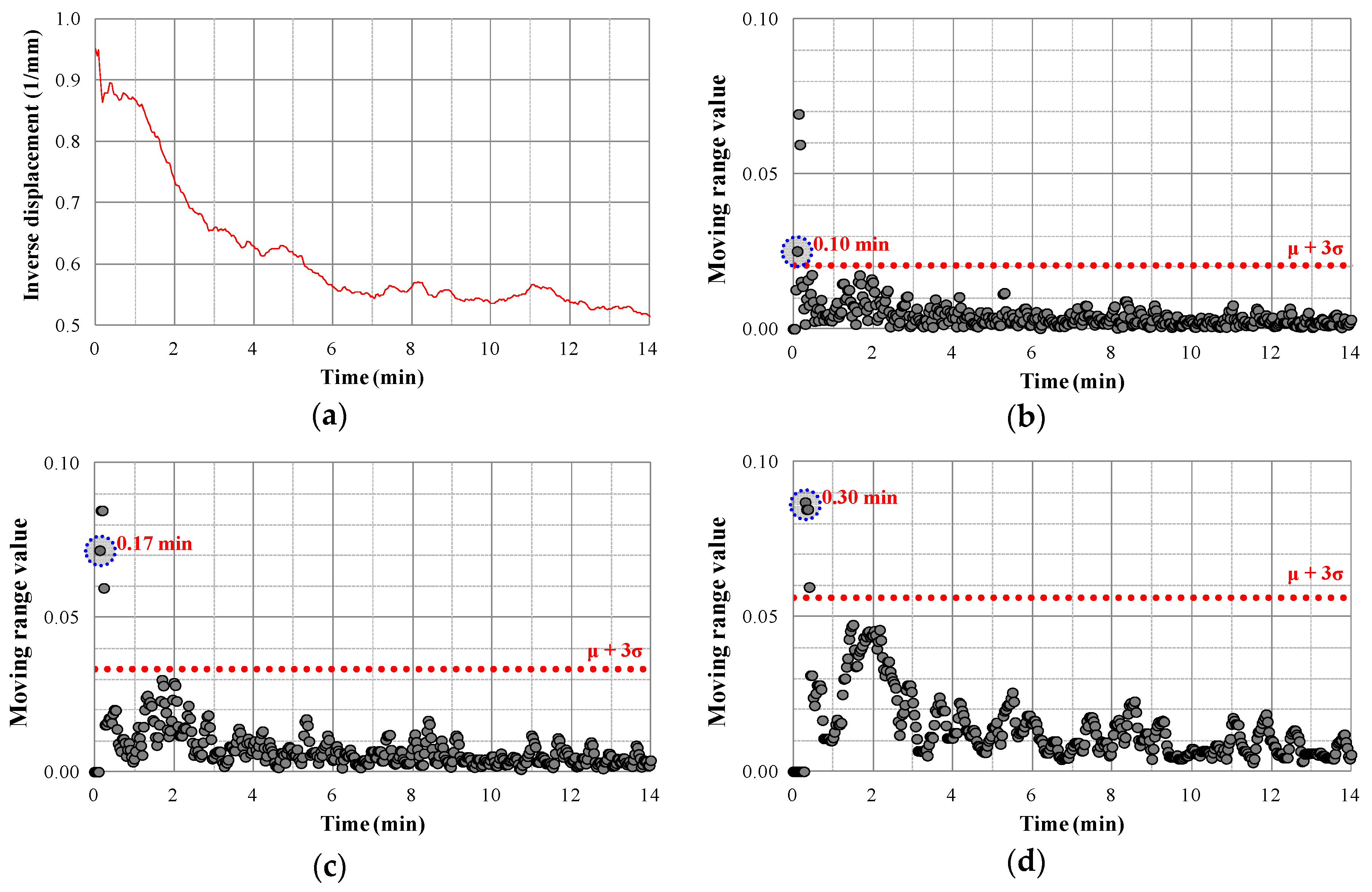
4.2. x–MR Control Chart Analysis
4.3. Proposal for Slope Instrumentation Standards
5. Conclusions
- (1)
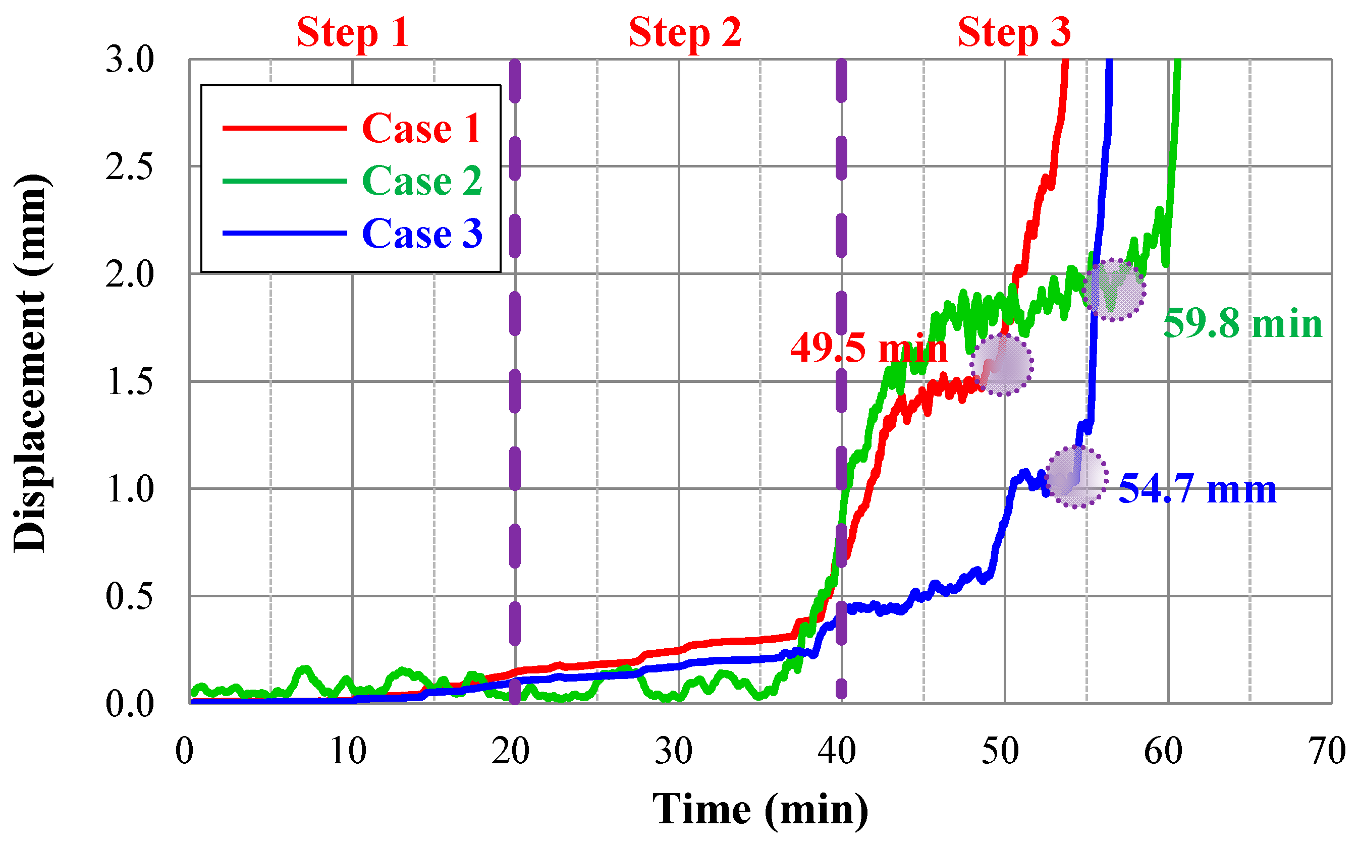
- As a result of the real scale slope failure model test, the final slope failure was confirmed in all the cases. However, the slope failure was predictable in cases 1 and 2 beforehand, in which the progressive failure that included displacement exceeding 1 mm was observed. However, in case 3, the pre-prediction was not possible prior to the slope failure.
- (2)
- Based on evaluation of the slope failure for various moving ranges (K) through an x–MR control chart on significant displacement data, it is concluded that applying K = 3 is effective.
- (3)
- The x–MR control approach of inverse displacement can be applied to make quick and objective decisions about slope failure behavior and for predicting slope failure.
- (4)
- It is considered that the analysis method of slope failure proposed through this study can increase the efficiency of the disaster management policy implementation for local government officials by providing more reliable risk assessment results, along with the steep slope failure prediction, early warning system, landslide information system, etc.
Supplementary Materials
Author Contributions
Funding
Acknowledgments
Conflicts of Interest
References
- Barredo, J.I. Normalised flood losses in Europe: 1970–2006. Nat. Hazards Earth Syst. Sci. 2009, 9, 97–104. [Google Scholar] [CrossRef]
- European Environment Agency. Mapping the Impacts of Natural Hazards and Technological Accidents in Europe. An Overview of the Last Decade; European Environment Agency: København, Denmark, 2010; ISBN 9789292131685. [Google Scholar]
- EM-DAT. The OFDA/CRED International Disaster Database; Université Catholique de Louvain: Brussels, Belgium; Available online: http://www.emdat.be/ (accessed on 6 August 2019).
- Alfieri, L.; Salamon, P.; Pappenberger, F.; Wetterhall, F.; Thielen, J. Operational early warning systems for water-related hazards in Europe. Environ. Sci. Policy 2012, 21, 35–49. [Google Scholar] [CrossRef]
- Piciullo, L.; Calvello, M.; Cepeda, J.M. Territorial early warning systems for rainfall-induced landslides. Earth-Sci. Rev. 2018, 179, 228–247. [Google Scholar] [CrossRef]
- Eun-Chul, S.; Kim, J.-I. Stability Analysis of Geocell Reinforced Slope During Rainfall. J. Korean Geosynth. Soc. 2017, 16, 33–41. [Google Scholar]
- Han, J.-G.; Hong, K.-K.; Lee, J.-Y.; Jung, S.-K. Application Evaluation of Countermeasure Method using Analysis of Failure Causes for Reinforced Slope. J. Korean Geosynth. Soc. 2011, 10, 9–18. [Google Scholar]
- Korea Institute of Geoscience and Mineral Resources. Development of an Integrated Early Detection System of Landslides Based on a Real-Time Monitoring; Research Institute Report: Gyeonggi-do, Korea, 2014. (In Korean) [Google Scholar]
- Wieczorek, G.; Snyder, J. Monitoring slope movements. Geol. Monit. 2009, 245–271. Available online: http://www.science.earthjay.com/instruction/chemeketa/2015_spring/GEO144/lectures/lecture_07/GEO144_lecture_7_Wieczorek_Snyder_2009_overview_monitoring_slope_movements.pdf (accessed on 2 July 2019).
- Keefer, D.K.; Wilson, R.C.; Mark, R.K.; Brabb, E.E.; Brown, W.M.; Ellen, S.D.; Harp, E.L.; Weiczorek, G.F.; Alger, C.S.; Zazkin, R.S. Real-Time Landslide Warning During Hearvy Rainfall. Science 1987, 238, 921–925. [Google Scholar] [CrossRef]
- Wilson, R.C. The Rise and Fall of a Debris-Flow Warning System for the San Francisco Bay Region, California. In Landslide Hazard and Risk; John Wiley & Sons: Hoboken, NJ, USA, 2012; pp. 493–516. ISBN 9780471486633. [Google Scholar]
- Godt, J.W.; Baum, R.L.; Chleborad, A.F. Rainfall characteristics for shallow landsliding in Seattle, Washington, USA. Earth Surf. Process. Landf. 2006, 31, 97–110. [Google Scholar] [CrossRef]
- Chleborad, A.F.; Baum, R.L.; Godt, J.W.; Powers, P.S. A prototype system for forecasting landslides in the Seattle, Washington, area. GSA Rev. Eng. Geol. 2008, 20, 103–120. [Google Scholar]
- Baum, R.L.; Godt, J.W. Early warning of rainfall-induced shallow landslides and debris flows in the USA. Landslides 2010, 7, 259–272. [Google Scholar] [CrossRef]
- Lari, S.; Frattini, P.; Crosta, G.B. A probabilistic approach for landslide hazard analysis. Eng. Geol. 2014, 182, 3–14. [Google Scholar] [CrossRef]
- Haneberg, W.C. A rational probabilistic method for spatially distributed landslide hazard assessment. Environ. Eng. Geosci. 2004, 10, 27–43. [Google Scholar] [CrossRef]
- Park, H.J.; Lee, J.H.; Woo, I. Assessment of rainfall-induced shallow landslide susceptibility using a GIS-based probabilistic approach. Eng. Geol. 2013, 161, 1–15. [Google Scholar] [CrossRef]
- Raia, S.; Alvioli, M.; Rossi, M.; Baum, R.L.; Godt, J.W.; Guzzetti, F. Improving predictive power of physically based rainfall-induced shallow landslide models: A probabilistic approach. Geosci. Model Dev. 2014, 7, 495–514. [Google Scholar] [CrossRef]
- Lee, J.H.; Park, H.J. Assessment of shallow landslide susceptibility using the transient infiltration flow model and GIS-based probabilistic approach. Landslides 2016, 13, 885–903. [Google Scholar] [CrossRef]
- Zhang, S.; Zhao, L.; Delgado-Tellez, R.; Bao, H. A physics-based probabilistic forecasting model for rainfall-induced shallow landslides at regional scale. Nat. Hazards Earth Syst. Sci. 2018, 18, 969–982. [Google Scholar] [CrossRef]
- Salciarini, D.; Fanelli, G.; Tamagnini, C. A probabilistic model for rainfall—Induced shallow landslide prediction at the regional scale. Landslides 2017, 14, 1731–1746. [Google Scholar] [CrossRef]
- Park, S.; Min, Y.; Kang, M.; Jung, H.; Sami, G.; Kim, Y. Slope Failure Prediction through the Analysis of Surface Ground Deformation on Field Model Experiment. J. Korean Geosynth. Soc. 2017, 16, 1–10. [Google Scholar]
- Sung-yong, P.; Hee-don, J.; Young-ju, K.; Yong-seong, K. A study on Behavior of Slope Failure Using Field Excavation Experiment. J. Korean Soc. Agric. Eng. 2017, 59, 101–108. (In Korean) [Google Scholar]
- Shewhart, W.A. Some Applications of Statistical Methods to the Analysis of Physical and Engineering Data. Bell Syst. Tech. J. 1924, 3, 43–87. [Google Scholar] [CrossRef]
- Kwon, O.; Baek, Y.; Seo, Y.S. Development of slope displacement data analysis system using control chart theory. In Proceedings of the Conference of the Korean Society of Engineering Geology, Cheongju, Korea, 6–7 November 2008; pp. 137–143. [Google Scholar]
- Yoo, B. A Study of Failure Analysis Methods Based on Real-Time Monitoring Data for Landslide Warning System. Ph.D. Dissertation, Graduate School Kumoh National Institute of Technology, Gumi, Korea, 2006. (In Korean). [Google Scholar]
- Yoo, B.S.; Park, Y.D.; Lee, K.S.; Chang, K.T. Failure Prediction and Analysis of Prone-landslide with x-MR Control Chart. In Proceedings of the 35th Korean Society of Civil Engineers Conference, Gangwon-do, Korea, 21–23 October 2009; Volume 10, pp. 1779–1802. (In Korean). [Google Scholar]
- Kim, S.B. Unstable Soil Behavior Detecting Methods in Flume Test Using Applied Statistical Analysis; Chungbuk National University: Cheongju, Korea, 2014. (In Korean) [Google Scholar]
- Koutras, M.V.; Bersimis, S.; Maravelakis, P.E. Statistical process control using shewhart control charts with supplementary runs rules. Methodol. Comput. Appl. Probab. 2007, 9, 207–224. [Google Scholar] [CrossRef]
- Yun, H.S.; Song, K.K.; Shin, Y.W.; Kim, C.Y.; Choo, S.Y.; Seo, S.S. Application of x-MR control chart on monitoring displacement for prediction of abnormal ground behaviour in tunnelling. J. Korean Tunn. Undergr. Space Assoc. 2014, 16, 445–458. [Google Scholar] [CrossRef]
- Yim, S.; Seo, Y.-S. A New Method for the Analysis of Measured Displacements during Tunnelling using Control Charts. J. Eng. Geol. 2009, 19, 261–268. [Google Scholar]
- Voight, B. A method for prediction of volcanic eruptions. Nature 1988, 332, 125–130. [Google Scholar] [CrossRef]
- Park, S.; Chang, D. Prediction of Slope Failure Using Control Chart Method. J. Korean Geosynth. Soc. 2018, 17, 9–18. [Google Scholar]
- Fukuzono, T. A Method to Predict the Time of Slope Failure Caused by Rainfall Using the Inverse Number of Velocity of Surface Displacement. Landslides 1985, 22, 8–13. [Google Scholar] [CrossRef]
- Tamate, S.; Hori, T.; Mikuni, C.; Suemasa, N. Experimental analyses on detection of potential risk of slope failure by monitoring of shear strain in the shallow section. In Proceedings of the 18th International Conference on Soil Mechanics and Geotechnical Engineering, Paris, France, 2–6 September 2013; pp. 1901–1904. [Google Scholar]
- Lee, J.D. The R&D Research on Construction of Monitoring Management System for Evacuation Inhabitant in Steep Slope Site and Development of Monitoring Specification; Disaster and Safety Management Institute: Sejong-si, Korea , May 2015. (In Korean) [Google Scholar]


| USCS | (kN/m3) | (kN/m3) | wopt (%) | Sand (%) | Silt (%) | Clay (%) | D50 (mm) |
|---|---|---|---|---|---|---|---|
| SW | 17.58 | 18.89 | 13.3 | 56.1 | 9.8 | 1.6 | 0.85 |
| Step | Displacement (s) (mm) | Time (t0) (min) | Control Limit | Phase |
|---|---|---|---|---|
| 1 | 0 < s < 1.0 | - | Safe | Normal Phase |
| 2 | 1.0 < s < 1.5 | 0.1 | Unsafe | Anomalous Phase |
| 3 | s > 1.5 | 7.7 | - | Failure Phase |
© 2019 by the authors. Licensee MDPI, Basel, Switzerland. This article is an open access article distributed under the terms and conditions of the Creative Commons Attribution (CC BY) license (http://creativecommons.org/licenses/by/4.0/).
Share and Cite
Park, S.; Lim, H.; Tamang, B.; Jin, J.; Lee, S.; Chang, S.; Kim, Y. Analysis of Slope Failure Behaviour Based on Real-Time Measurement Using the x–MR Method. J. Mar. Sci. Eng. 2019, 7, 360. https://doi.org/10.3390/jmse7100360
Park S, Lim H, Tamang B, Jin J, Lee S, Chang S, Kim Y. Analysis of Slope Failure Behaviour Based on Real-Time Measurement Using the x–MR Method. Journal of Marine Science and Engineering. 2019; 7(10):360. https://doi.org/10.3390/jmse7100360
Chicago/Turabian StylePark, Sungyong, Hyuntaek Lim, Bibek Tamang, Jihuan Jin, Seungjoo Lee, Sukhyun Chang, and Yongseong Kim. 2019. "Analysis of Slope Failure Behaviour Based on Real-Time Measurement Using the x–MR Method" Journal of Marine Science and Engineering 7, no. 10: 360. https://doi.org/10.3390/jmse7100360
APA StylePark, S., Lim, H., Tamang, B., Jin, J., Lee, S., Chang, S., & Kim, Y. (2019). Analysis of Slope Failure Behaviour Based on Real-Time Measurement Using the x–MR Method. Journal of Marine Science and Engineering, 7(10), 360. https://doi.org/10.3390/jmse7100360