Direct Measurements of Bed Shear Stress under Swash Flows on Steep Laboratory Slopes at Medium to Prototype Scales

Abstract

Robust measurements of bed shear stress under wave runup flows are necessary to inform beachface sediment transport modelling. In this study, direct measurements of swash zone bed shear stress were obtained in medium and prototype-scale laboratory experiments on steep slopes. Peak shear stresses coincided with the arrival of uprush swash fronts and high-resolution measurement of swash surface profiles indicated a consistently seaward sloping swash surface with minimal evidence of a landward sloping swash front. The quadratic stress law was applied to back-calculate time-varying friction factors, which were observed to decrease with increasing Reynolds number on smooth slopes, consistent with theory for steady flows. Additionally, friction factors remained relatively constant throughout the swash cycle (except around flow reversal), with a variation of approximately ±20% from the mean value and with only small differences between uprush and backwash. Measured friction factors were observed to be larger than expected when plotted on the Moody or wave friction diagram for a given Reynolds number and relative roughness, consistent with previous field and laboratory studies at various scales.

1. Introduction

When a fluid flows past a solid boundary, shear stresses are generated. For rough, fully developed turbulent flows, bed shear stress, τ₀, is commonly related to a friction factor, f, through the quadratic stress law, adapted from the Rayleigh (1876) drag equation [1]:

$${\tau }_0=\frac{1}{2}\rho f\left|U\right|U$$

(1)

where ρ is fluid density and U is the depth-averaged flow velocity. This formulation is well established for calculating bed shear stress in steady, uniform flow conditions, where f remains constant (e.g., [2,3]). It has also been widely adopted to describe hydrodynamics in the swash zone, where unsteady conditions prevail.

Previous authors have used a range of direct and indirect measurement techniques to calculate friction factors in swash flows (a summary of selected studies is presented in

Table 1. Experimental conditions and instrumentation from selected previous studies.

Study	Roughness (mm)	Slope	Study Type	Primary Measurement Technique
Hughes (1995) [8]	0.3–2.0	1:11–1:7	Field	Capacitance gauge
Cox et al. (2000) [6]	6.3	1:10	Laboratory	Laser Doppler velocimetry
Puleo and Holland (2001) [9]	0.26, 0.35, 0.44	1:12	Field	Video camera
Cowen et al. (2003) [7]	Smooth	1:20	Laboratory	Particle image velocimetry
Conley and Griffin (2004) [5]	Medium sand	Dissipative	Field	Hot film anemometer
Barnes et al. (2009) [10]	0.2, 5.8	1:12, 1:10	Laboratory	Shear plate
Kikkert et al. (2012) [11]	1.3, 5.5, 8.4	1:10	Laboratory	Particle image velocimetry
Puleo et al. (2012) [12]	0.2, 0.25	1:20	Field	Acoustic Doppler profiler
Inch et al. (2015) [13]	0.33	1:40	Field	Acoustic Doppler profiler
Pujara et al. (2015) [14]	Smooth plywood	1:12	Laboratory	Shear plate

and Figure 1), but the results vary widely between studies (see review [4]), with mean values ranging from f = 0.001 [5] to f = 0.04 [6]. Furthermore, previous studies have often found f to differ between uprush and backwash, and even to vary continuously through the swash cycle (e.g., [7]).

If swash flows are approximated as steady uniform flows in a channel of infinite width, a friction factor can be calculated by applying the Colebrook–White equation [15]:

$$\frac{1}{\sqrt{\lambda }}=-2{\mathit{log}}_{10}\left(\frac{k_s}{3.7D_H}+\frac{2.51}{Re\sqrt{\lambda }}\right)$$

(2)

where λ is the Darcy friction factor [16], related to the Fanning) friction factor [17], f, by λ = 4f, while k_s is sand grain roughness, D_H is hydraulic diameter (D_H = 2h for wide rectangular channels, where h is depth), and Re is Reynolds number [18], given by:

$$Re=\frac{uD}{\nu }$$

(3)

where u is a characteristic fluid velocity, and ν is kinematic viscosity (ν = 10⁻⁶ m²/s for water).

Numerical models of the nearshore environment typically assume f remains constant through the swash cycle (e.g., [19]). That assumption was tested in this investigation, by back-calculating values of f via the quadratic stress law, using depth-averaged velocity and direct measurements of bed shear stress (provided with a flush-mounted shear plate).

2. Materials and Methods

The results discussed below were obtained through two laboratory experiments in medium and prototype-scale facilities. Both experiments were performed on steep, impermeable slopes. All runup observations from both experiments are reported in bed-parallel coordinates.

2.1. UNSW Water Research Laboratory (WRL)—Medium Scale

One set of experiments was performed using a wave flume (30 m long and 3 m wide) at the Water Research Laboratory (WRL), a facility of the School of Civil and Environmental Engineering, UNSW Sydney, Australia. A 1:3 plywood slope was constructed approximately 8 m from the piston-type wave paddle on top of an existing flat bathymetry with a 1:10 slope at the toe (Figure 2). The water depth was 0.68 m. Water levels were measured using a capacitance wave gauges, and incident and reflected wave spectra were separated using the Mansard and Funke (1980) method [20]. Swash depths were measured using an array of eight Microsonic mic+35 ultrasonic sensors mounted perpendicular to the bed, and spaced at approximately 0.25 m intervals. Bed shear stress was measured with a flush-mounted shear plate [21], with a displacement sensor accuracy of ≤2%. The instruments were connected to a data acquisition PC sampling at 200 Hz for the shear plate, and 40 Hz for the ultrasonic altimeters.

Depth-averaged fluid velocities were calculated using the volume continuity method ([22,23]) based on incremental changes in the measured time-varying swash volume under the ultrasonic sensor array. These continuity-derived velocities had an effective spatial resolution of 0.25 m and a temporal resolution of 200 Hz. Protracted efforts were made to measure swash velocities directly using an electromagnetic current meter mounted close to the bed, but the data were discarded because the instrument did not perform well with the shallow, intermittent flows.

A test program of monochromatic waves was developed, attempting to maximise the range of wave steepness values. Breaker type is generally related to wave steepness using the surf similarity parameter, ξ₀ [24]:

$${\xi }_0=\frac{\tan \beta }{\sqrt{H/L_0}}$$

(4)

where β is beach slope, H is wave height, and L₀ is deep water wavelength. Because of the small waves and steep slope used in the WRL experiments, it was more practical to classify the breaker types qualitatively from video records, instead of directly calculating ξ₀.

The test program (

Table 2. Test program, WRL experiments.

Test	Wave Type	T (s)	H (m)	Breaker Type	Dmax (m)	Umax (m/s)	Remax
1	Monochromatic	2.2	0.11	Plunging	0.05	2.0	1.4 × 105
2	Monochromatic	3.2	0.22	Plunging	0.07	2.0	2.3 × 105
3	Monochromatic	3.2	0.16	Collapsing	0.06	1.7	1.3 × 105
4	Monochromatic	5.0	0.16	Collapsing	0.11	2.2	2.1 × 105

) was repeated four times. The conditions for each repeat were identical, except that the shear plate was installed in a different cross-shore position (A, B, C, and D, in Figure 1) to quantify the spatial variation in bed shear stress. The position of the ultrasonic sensors was modified slightly between each test series, so that two sensors were always located directly above the landward and seaward edge of the shear plate. The most seaward sensor was kept in the same position for all tests to provide a constant reference.

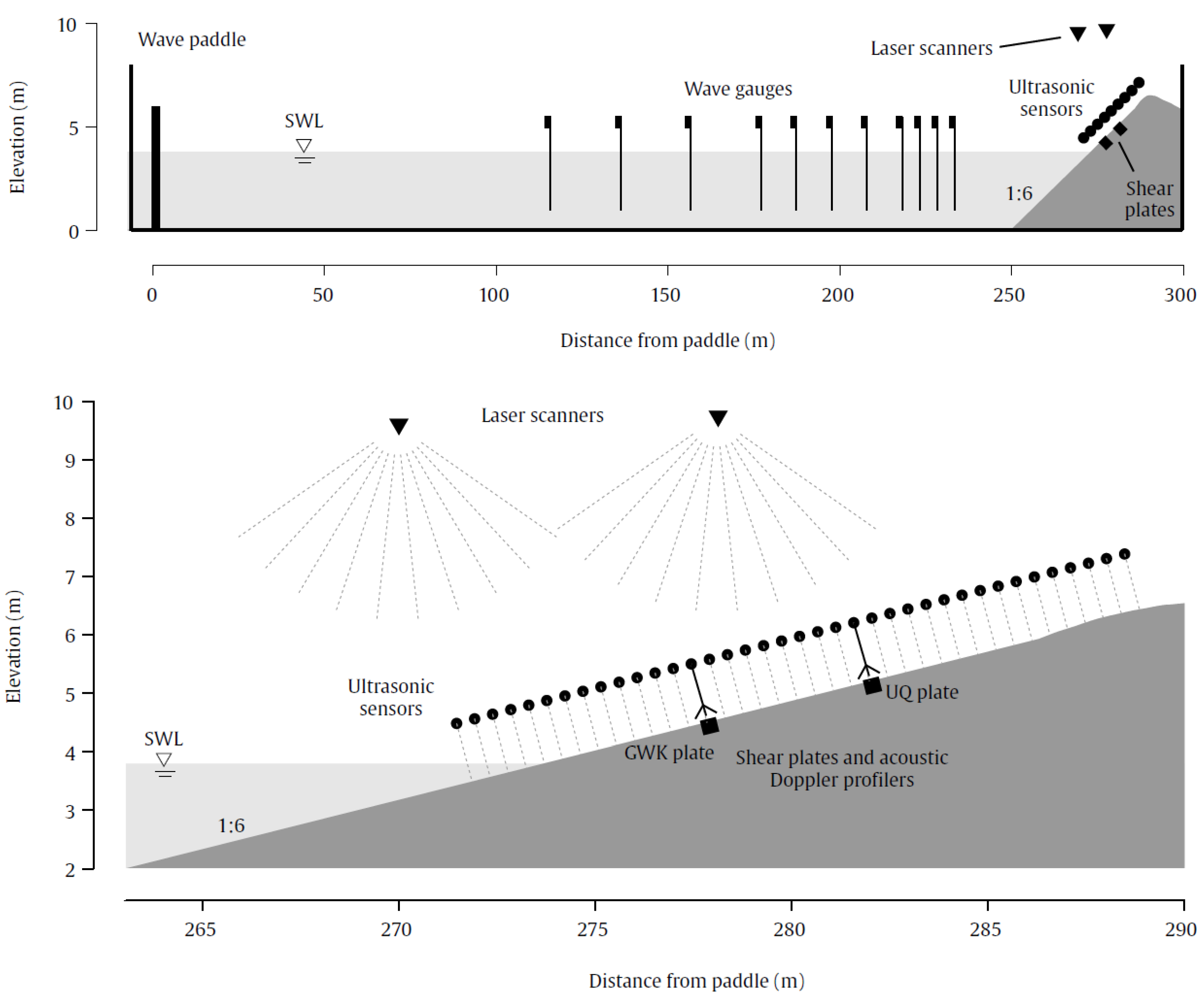
2.2. Große Wellenkanal (GWK)—Prototype Scale

A second set of experiments was performed in the Großer Wellenkanal (large wave flume; GWK) at prototype scale. GWK is 310 m long, 5 m wide, and is part of the Forschungzentrum Küste (Coastal Research Centre; FZK) in Hanover, Germany. For this experiment, the instruments were installed on a 1:6 slope, approximately 280 m from the piston-type wave paddle (Figure 3). The water depth was 3.8 m.

Wave heights were measured with resistance-type wave gauges sampled at 120 Hz, and instantaneous water depths in the swash zone were provided by an array of 41 Massa M300/95 ultrasonic altimeters sampling at 4 Hz, and mounted to a scaffolding rig at 0.4 m cross-shore intervals at a height of approximately 1 m. The ultrasonic altimeters were supplemented by four laser scanners mounted on two separate crane trolleys suspended above the centre of the flume at distances of 3.5 m offshore, and 4.6 m onshore of the intersection between the still water level and the beach. One SICK LMS511 and one FARO FOCUS 3D 120S laser scanner were mounted on each trolley, and these instruments were sampled at 35 Hz and 24 Hz, respectively and used to measure time-varying free-surface elevation throughout the inner surf and swash zones (e.g., [25]). Fluid velocities were measured at two cross-shore locations with Vectrino II acoustic Doppler profilers, sampled at 100 Hz.

Depth-averaged fluid velocities were also calculated across the entire swash zone using the volume continuity method from ultrasonic altimeter measurements, yielding an effective spatial resolution of 1 m, and a temporal resolution of 4 Hz. These depth-averaged velocities were validated with the acoustic Doppler profilers, and with laser scanner measurements of the swash leading edge during uprush (Figure 4).

Two shear plates were installed flush with the bed at different cross-shore positions (co-located with the acoustic Doppler profilers), both sampled at 120 Hz (Figure 5). A new bed shear stress transducer (hereafter the GWK shear plate) was used alongside the Barnes and Baldock (2006) [21] instrument (hereafter the University of Queensland (UQ) shear plate). The active face of the GWK shear plate consists of an aluminium disc with a diameter of 150 mm. A flexible rubber gasket sits between the active face and the housing to ensure the shear plate is hermetically sealed (in contrast to the UQ plate). Two dual-beam load cells provide bed shear stress measurements in the x and y directions, with an accuracy of 0.04% [26]. The GWK shear plate and the UQ shear plate were located at distances of 4.4 m and 8.3 m from intersection with the still water level, respectively. A video camera with a wide-angle lens was mounted on the seaward trolley to visually record the swash flows.

A total of 12 monochromatic and irregular (JONSWAP) wave tests were recorded with significant wave height (H_s) between 0.6 m and 1.0 m, and peak wave period (T_p) ranging from 8 s to 14 s (

Table 3. Test program, GWK experiments. Note that peak period (T_p) and significant wave height (H_s) are shown for irregular wave cases.

Rough Tests	Smooth Tests	Wave Type	T (s) 1	H (m) 1	ξ0	Breaker Type	Dmax (m) 2	Umax (m/s) 2	Remax 2
R1	S1	Monochromatic	8.0	0.88	1.8	Plunging	0.28	5.4	1.2 × 106
	S2	Monochromatic	8.0	0.99	1.7	Plunging	0.32	4.9	1.3 × 106
	S3	Monochromatic	10.0	0.97	2.1	Plunging	0.33	4.3	1.6 × 106
	S4	Monochromatic	12.0	0.61	3.2	Plunging	0.32	3.8	1.2 × 106
	S5	Monochromatic	12.0	0.72	3.0	Plunging	0.35	5.0	1.7 × 106
R2	S6	Monochromatic	12.0	0.95	2.6	Plunging	0.43	5.6	2.0 × 106
	S7	Monochromatic	14.0	0.63	3.8	Collapsing	0.35	3.7	1.2 × 106
	S8	Monochromatic	14.0	0.85	3.3	Plunging	0.44	4.5	2.1 × 106
R3	S9	Irregular 3	12.0	0.82	2.8	Plunging	0.28	5.2	9.8 × 105
1. Measured offshore (120 m from paddle). 2. Measured in swash zone (above GWK shear plate).

). The experiments were performed on two different surfaces of contrasting roughness: a ‘rough’ asphalt surface (tests R1–R2) and a ‘smooth’ polyethylene surface (tests S1–S9). The surface of each shear plate was carefully prepared to closely match the roughness of the surrounding slope. The sand grain roughness of both shear plates was taken as k_s = 0.003 mm for the smooth surface experiments, based on the recommended value for smooth aluminium [27]. During the rough surface experiments, polyurethane moulds of the asphalt surface were glued to the shear plates (Figure 5). Based on photographs and a high-resolution 3D laser survey of the asphalt surface, a roughness value of k_s = 1.5 mm was used for the rough surface experiments.

3. Results

A rich dataset of direct bed shear stress measurements was collected during the WRL and GWK experiments. The shear plates were deployed in multiple locations across the beachface under a wide range of incident wave conditions, allowing bed shear stress to be compared with several other parameters, including bed roughness, experimental scale and cross-shore location.

3.1. Swash Surface Profiles and Boundary Layer Development

Figure 6 illustrates concurrent measurements of the water depth, pressure gradient and bed shear stress, and three snapshots of the water surface profile as a swash front passes the shear plate for monochromatic wave case S2. The water surface profiles are derived from the laser scanner systems positioned above the flume and the data presented are raw data without filtering. The pressure gradient is consistent with that previously observed by Barnes et al. (2009) [10], indicating a water surface dipping seaward, and also documented in field observations [28]. As the swash front passes the shear plate, the well-known immediate spike in the shear stress occurs, but the water surface profile shows little indication of a significant rounded swash front. Thus, there is little evidence that the spike in shear stress and rapid decay is a consequence of, or leads to, the formation of a bull-nose profile at the wave tip, as proposed by [29] on the basis of Eulerian measurements of the flow depth at a point. Indeed, as argued by [30], timeseries measurements of water depth at a fixed point provide little or misleading information about the water surface profile since the swash is unsteady. Consistent with previous data that points to the presence of a well-developed boundary layer at the swash tip (see [30] and [31]), as opposed to a boundary layer growing from the swash tip [29], acoustic Doppler profiler measurements from the GWK experiment show that the boundary layer is at its most fully developed state at the leading edge of the swash, see Figure 7. This is consistent with the boundary layer growing as the flow proceeds up the beach, with the flow at the free surface converging on the front, and with the high shear stress a result of the shallow flow (thin overall boundary layer) and the injection of higher velocity fluid at the wave tip [32].

3.2. Influence of Bed Roughness on Bed Shear Stress

The GWK experiments were performed on contrasting rough asphalt and smooth polyethylene surfaces. The UQ shear plate was used to measure bed shear stress for the two different surfaces under the same monochromatic wave conditions (Figure 8). As expected, the bed shear stress magnitude over all test cases was larger on the rough surface (by 80% to 100% for uprush and 40% to 60% for backwash). The key feature of larger stresses during uprush is consistent with previous data. The peak backwash bed shear also occurs earlier in the swash cycle for the rough case, compared to the smooth case. This backwash peak is probably caused by the transition to a turbulent boundary layer [32]. The larger peaks on the rough surface may have also been partially caused by the gap (approximately 5 mm wide) between the moulded roughness element attached to the UQ shear plate and the surrounding fixed bed (Figure 5). The gap was kept as small as possible while still allowing free movement of the plate, but may have contributed additional form drag into the bed shear stress measurements. The roughness element interfered with the operation of the GWK shear plate, causing it to produce spurious measurements (which were discarded).

3.3. Influence of Cross-shore Position on Bed Shear Stress

Cox et al. [6], Barnes et al. [10], and Sumer et al. [33] measured the cross-shore variation in swash zone bed shear stress, and all found τ_o to reach a maximum slightly landward of the still water level, reducing to zero near the maximum uprush limit. Bed shear stress was measured at four different positions on the beachface during the WRL experiments, and the cross-shore bed shear stress envelope (peak value at each location) was calculated for three different monochromatic wave cases (Figure 9). The envelope was normalised with respect to both the peak uprush bed shear, τ_o,maz, and the maximum uprush limit, R_x.

The WRL bed shear stress measurements showed good agreement with previous studies for the uprush phase, but were proportionally larger during backwash (Figure 10). These backwash bed shear stresses appear larger because they are scaled based on τ_o,max in the uprush phase. The waves in the WRL experiments were generally collapsing. Under these conditions, a relatively large portion of the swash cycle consists of the bore collapse process (where the fluid is accelerating), so τ_o,max occured higher up the beachface. The general factor two difference in the peak stresses between uprush and backwash is explained by the Lagrangian Boundary layer model of Barnes and Baldock [32], whereas the model of Nielsen [34] predicts larger shear stress in the backwash where the backwash is decelerating.

3.4. Friction Factors

The effective Fanning friction factor for the WRL and GWK experiments was back calculated from time-varying depth-averaged velocity and bed shear stress measurements at each shear plate location, using the quadratic stress law:

$$f\left(t\right)=\frac{2\tau \left(t\right)}{\rho \left|U\left(t\right)\right|U\left(t\right)}$$

(5)

Friction factors calculated in this way tend to approach infinity close to flow reversal, because the divisor is close to zero. For the purposes of this analysis, friction factors were not calculated when velocities were small (|U| < 0.5 m/s). Flow reversal occurred rapidly (and the phase discrepancy between τ_o and U was small) because of the steep slopes used in this investigation. Velocities were large. Maximum depth-averaged velocities calculated using the ultrasonic altimeters regularly exceeded 4 m/s in both uprush and backwash during the GWK experiments—larger than velocities reported in previous studies [4].

The period where |U| < 0.5 m/s accounted for 20%−25% and 10%−20% of the swash duration for the WRL and GWK experiments, respectively. Bed shear stress was at a minimum in this region: less than 10%−20% of τ_o,max for the WRL experiments, and less than 10%−15% of τ_o,max for the GWK experiments. The time-integrated bed shear stress (i.e., the effective sediment transport potential) around flow reversal was less than 5% of the total.

3.4.1. Friction Factors (WRL Experiment)

The mean value of f was found to be approximately 0.01 for the WRL experiments (Figure 11), and remained fairly constant with time, with a variation of approximately ±40% from the mean value during the backwash phase. This is more consistent than previous studies, some of which present f values on a log scale.

Friction factors were generally highest in the mid-swash zone (Figure 12). There was little variation between uprush and backwash, with the exception of test case 4 (Table 1, H = 0.16 m, T = 5 s), where f was 2−3 times larger during backwash. This is in contrast to some previous studies which have observed significant differences between estimated friction factors during uprush and backwash (Figure 1).

3.4.2. Friction Factors (GWK Experiment)

The mean value of f for the GWK experiments was found to be approximately 0.005 for the smooth surface and 0.008 for the rough surface (Figure 13), with 50% of instantaneous values within ±0.0015 and ±0.0025, respectively. On the smooth surface, f remained fairly constant with time for incident waves of varying height (Figure 14), and period (Figure 15), and were observed to be comparable during uprush and backwash. Friction factors were also calculated for a selection of irregular waves from the smooth surface experiments (Figure 16). The friction factors showed more variability within swash cycles than the ensemble-average cases, but the mean value was similar.

Sediment transport models typically use a constant f for convenience and due to the lack of certainty in the time-varying behavior of this parameter. The calculated friction factors from the GWK and WRL experiments tend to increase around flow reversal, consistent with other studies (e.g., [6,10,14]). This apparent increase in f may be an artefact of division by zero, or incorrect application of (5) because there is no longer fully developed turbulent flow when velocities are small close to flow reversal. If the region close to flow reversal is ignored, f remains relatively constant through the swash cycle in the current experiments. Thus, it appears that the use of a constant value of f is not unreasonable, and because sediment transport models typically use velocity raised to the second or third power [35], any variability in f is likely to have only a secondary effect on calculated transport rates.

3.4.3. Comparison of measured friction factors with previous studies

Typical friction factors for swash uprush from previous work have been collated and plotted on both the Moody diagram (Darcy friction factors) (Figure 16) and the wave friction factor diagram ([36], Figure 17), with the data from this study also added. As expected, the friction factor was observed to decrease with increasing Reynolds number; however, wave friction factors at the same Reynolds numbers (which are defined differently in the two approaches as detailed in the figure captions) are typically 5–10 times larger than Darcy friction factors, which is not completely explained by the factor 4 difference in the definition of f. In both plots, typical friction factors in the uprush are larger than expected for steady uniform flows with the same value of the relative roughness at a given Reynolds number in the current study. This is explained in part by the fact that the uprush flows are unsteady and exhibit a developing boundary layer and flow convergence at the swash tip leading to enhanced bed shear stress. This trend also holds true for all previous studies except point number 3 (Conley and Griffin [5]). Conley and Griffin [5] used a very different measurement approach to all other studies and their results are notably inconsistent with other reported datasets. It is also observed that on the wave friction plot (Figure 17), the result of Cowen et al. [7] plots outside the valid range found by [36] due to the low Reynolds number of the measured flow. For the prototype-scale GWK experiments, it was found that the Colebrook–White equation (Moody diagram) can be used to estimate time-varying friction factors to an accuracy of ±50% if a constant roughness height is applied; however, higher errors (up to approximately 600%) are observed for the other studies.

4. Conclusions

This paper presents the first direct, prototype-scale measurements of bed shear stress in the swash zone obtained using a shear plate. Data were collected on both smooth and rough surfaces. Analysis of swash surface profiles confirmed previous observations of a consistently off-shore sloping swash surface except in the few centimetres behind the leading edge of the swash. Arrival of the swash front coincided with the maximum measured shear stress, associated with a well-developed boundary layer at the swash tip. Peak uprush bed shear stresses were found to be typically 2 times greater than during the backwash, with the largest values occurring in the lower/mid swash, landward of the initial bore collapse region. Peak shear stresses were greater for the rough surface by approximately 90% (50%) for uprush (backwash) flows and peak backwash shear stress consistently earlier in the rough bed case, likely caused by an earlier transition to a turbulent boundary layer.

Friction factors were back-calculated using the quadratic stress law, and were found to remain fairly constant (±20% from the mean value) during uprush and backwash, except around flow reversal. This result adds further evidence to support the applicability of the quadratic stress law for swash flows (enabling bed shear stress under wave runup to be approximated by using depth-averaged velocities, and ignoring fluid boundary layers).

Friction factor values were plotted on the Moody and wave friction factor diagram of Kamphuis (1975) along with the results of previous studies. Measured friction factors were observed to decrease with increasing Reynolds numbers as expected for steady, uniform flows. However, it was found that measured friction factors were larger than the values obtained from either plot for a given Reynolds number and relative roughness.

References

1. Rayleigh, L. On the resistance of fluids. Lond. Edinb. Dublin Philos. Mag. J. Sci. 1876, 2, 430–441. [Google Scholar] [CrossRef]
2. Putnam, J.; Johnson, J. The Dissipation of Wave Energy by Bottom Friction. Trans. Am. Geophys. Union 1949, 30, 67–74. [Google Scholar] [CrossRef]
3. Jonsson, I.G. Wave boundary layers and friction factors. In Proceedings of the 10th International Conference on Coastal Engineering, Tokyo, Japan, 4–6 September 1966; ASCE: New York, NY, USA, 1966; pp. 127–148. [Google Scholar]
4. Chardón-Maldonado, P.; Pintado-Patiño, J.C.; Puleo, J.A. Advances in swash-zone research: Small-scale hydrodynamic and sediment transport processes. Coast. Eng. 2015, 115, 8–25. [Google Scholar] [CrossRef]
5. Conley, D.C.; Griffin, J.G. Direct measurements of bed stress under swash in the field. J. Geophys. Res. 2004, 109, C03050. [Google Scholar] [CrossRef]
6. Cox, D.T.; Hobensack, W.; Sukumaran, A. Bottom Stress in the Inner Surf and Swash Zone. In Proceedings of the 27th International Conference on Coastal Engineering, Sydney, Australia, 16–21 July 2000; ASCE: New York, NY, USA, 2000; pp. 108–119. [Google Scholar]
7. Cowen, E.A.; Sou, I.M.; Liu, P.L.F.; Raubenheimer, B. Particle Image Velocimetry Measurements within a Laboratory-Generated Swash Zone. J. Eng. Mech. 2003, 129, 1119–1129. [Google Scholar] [CrossRef]
8. Hughes, M.G. Friction factors for wave uprush. J. Coast. Res. 1995, 4, 1089–1098. [Google Scholar]
9. Puleo, J.A.; Holland, K.T. Estimating swash zone friction coefficients on a sandy beach. Coast. Eng. 2001, 43, 25–40. [Google Scholar] [CrossRef]
10. Barnes, M.P.; O’Donoghue, T.; Alsina, J.M.; Baldock, T.E. Direct bed shear stress measurements in bore-driven swash. Coast. Eng. 2009, 56, 853–867. [Google Scholar] [CrossRef] [Green Version]
11. Kikkert, G.A.; O’Donoghue, T.; Pokrajac, D.; Dodd, N. Experimental study of bore-driven swash hydrodynamics on impermeable rough slopes. Coast. Eng. 2012, 60, 149–166. [Google Scholar] [CrossRef]
12. Puleo, J.A.; Lanckriet, T.M.; Wang, P. Near bed cross-shore velocity profiles, bed shear stress and friction on the foreshore of a microtidal beach. Coast. Eng. 2012, 68, 6–16. [Google Scholar] [CrossRef]
13. Inch, K.; Masselink, G.; Puleo, J.A.; Russell, P.E.; Conley, D.C. Vertical structure of near-bed cross-shore flow velocities in the swash zone of a dissipative beach. Cont. Shelf Res. 2015, 101, 98–108. [Google Scholar] [CrossRef] [Green Version]
14. Pujara, N.; Liu, P.L.-F.; Yeh, H. The swash of solitary waves on a plane beach: Flow evolution, bed shear stress and run-up. J. Fluid Mech. 2015, 779, 556–597. [Google Scholar] [CrossRef]
15. Colebrook, C.F. Turbulent flow in pipes, with particular reference to the transition region between the smooth and rough pipe laws. J. ICE 1939, 11, 133–156. [Google Scholar] [CrossRef]
16. Darcy, H. Recherches Expérimentales Relatives au Mouvement de L’eau Dans les Tuyaux (Experimental Research on the Movement of Water in the Pipes); Mallet-Bachelier: Paris, France, 1857. [Google Scholar]
17. Fanning, J.T. A Practical Treatise on Hydraulic and Water Supply Engineering; D. Van Norstrand Company: New York, NY, USA, 1893. [Google Scholar]
18. Reynolds, O. An experimental investigation of the circumstances which determine whether the motion of water shall be direct or sinuous, and of the law of resistance in parallel channels. Philos. Trans. R. Soc. 1883, 174, 935–982. [Google Scholar]
19. Roelvink, D.; Reniers, A.; van Dongeren, A.; van Thiel de Vries, J.; McCall, R.; Lescinski, J. Modelling storm impacts on beaches, dunes and barrier islands. Coast. Eng. 2009, 56, 1133–1152. [Google Scholar] [CrossRef]
20. Mansard, E.; Funke, E. The measurement of incident and reflected spectra using a least squares method. In Proceedings of the 17th International Conference on Coastal Engineering, Sydney, Australia, 23–28 March 1980; ASCE: New York, NY, USA, 1980; pp. 154–172. [Google Scholar]
21. Barnes, M.P.; Baldock, T.E. Bed shear stress measurements in dam break and swash flows. In International Conference on Civil and Environmental Engineering; Hiroshima University: Hiroshima, Japan, 2006. [Google Scholar]
22. Baldock, T.E.; Holmes, P. Swash hydrodynamics on a steep beach. In Proceedings of the Third Coastal Dynamics Conference, Plymouth, UK, 23–27 June 1997. [Google Scholar]
23. Blenkinsopp, C.E.; Turner, I.L.; Masselink, G.; Russell, P.E. Validation of volume continuity method for estimation of cross-shore swash flow velocity. Coast. Eng. 2010, 57, 953–958. [Google Scholar] [CrossRef]
24. Battjes, J.A. Surf similarity. In Proceedings of the 14th International Conference on Coastal Engineering, Copenhagen, Denmark, 24–28 June 1974; ASCE: New York, NY, USA, 1974. [Google Scholar]
25. Martins, K.; Blenkinsopp, C.E.; Power, H.E.; Bruder, B.; Puleo, J.A.; Bergsma, E. High-resolution monitoring of wave transformation in the surf zone using a LiDAR scanner array. Coast. Eng. 2017, 128, 37–43. [Google Scholar] [CrossRef]
26. Pero. Schubspannungsmesser Für den Einsatz am Meeresgrund (Shear Stress Plate for Use on the Seabed); PERO Gesellschaft für Meß und Steuertechnik GmbH: Sickte, Germany, unpublished work; 2007. (In German) [Google Scholar]
27. Barr, D.I.H. Tables for the Calculation of Friction in Internal Flows; Thomas Telford Publishing: London, UK, 1995. [Google Scholar]
28. Baldock, T.E.; Hughes, M.G. Field observations of instantaneous water slopes and horizontal pressure gradients in the swash zone. Cont. Shelf Res. 2006, 26, 574–588. [Google Scholar] [CrossRef]
29. Neilsen, P. Bed shear stress, surface shape and velocity field near the tips of dam-breaks, tsunami and wave runup. Coast. Eng. 2018, 138, 126–131. [Google Scholar] [CrossRef] [Green Version]
30. Baldock, T.E. Bed shear stress, surface shape and velocity field near the tips of dam-breaks, tsunami and wave runup. Discussion. Coast. Eng. 2018, 142, 77–81. [Google Scholar] [CrossRef]
31. Briganti, R.; Dodd, N.; Pokrajac, D.; O’Donohugh, T. Non linear shallow water modelling of bore-driven swash: Description of the bottom boundary layer. Coast. Eng. 2011, 58, 463–477. [Google Scholar] [CrossRef]
32. Barnes, M.P.; Baldock, T.E. A Lagrangian model for boundary layer growth and bed shear stress in the swash zone. Coast. Eng. 2010, 57, 385–396. [Google Scholar] [CrossRef]
33. Sumer, B.M.; Sen, M.B.; Karagali, I.; Ceren, B.; Fredsøe, J.; Sottile, M.; Zilioli, L.; Fuhrman, D.R.H. Flow and sediment transport induced by a plunging solitary wave. J. Geophys. Res. 2011, 116, C01008. [Google Scholar] [CrossRef]
34. Nielsen, P. Shear stress and sediment transport calculations for swash zone modelling. Coast. Eng. 2002, 45, 53–60. [Google Scholar] [CrossRef]
35. Nielsen, P. Coastal Bottom Boundary Layers and Sediment Transport; World Scientific: Singapore, 1992. [Google Scholar]
36. Kamphuis, J.W. Friction factor under oscillatory waves. J. Waterw. Port C-ASCE 1975, 101, 135–144. [Google Scholar]
37. Davis, T.G. Moody Diagram. MATLAB Central File Exchange. Available online: https://www.mathworks.com/matlabcentral/fileexchange/7747-moody-diagram (accessed on 1 October 2019).
Figure 1. Estimates Darcy friction factor f from current investigation (grey) and selected previous studies of swash flows in fixed-bed laboratory experiments (open symbols) and mobile bed field experiments (filled symbols), showing variation between uprush (△/▽), and backwash (▲/▼), where reported. ∗ indicates studies where f was calculated using observations of the leading/trailing edge of the swash, rather than the internal flow.
Jmse 07 00358 g001
Figure 2. Experimental setup, WRL.
Jmse 07 00358 g002
Figure 3. (Upper) Experimental setup, Große Wellenkanal (GWK); (lower) close-up of instrumentation on the subaerial slope.
Jmse 07 00358 g003
Figure 4. Example comparison of depth-averaged velocities, U derived from acoustic altimeters (black line), an acoustic Doppler profiler 20 mm above the bed (o) and the swash leading edge velocity, u (▽) measured using a laser scanner for four irregular waves during the GWK experiment.
Jmse 07 00358 g004
Figure 5. (a) GWK shear plate setup for smooth bed tests; (b) UQ shear plate with moulded rough surface.
Jmse 07 00358 g005
Figure 6. (a) Water depth (solid) and pressure gradient (dashed) measured during a single swash event during the GWK experiment for a monochromatic test case S2 (H = 0.99 m, T = 8 s) (b) bed shear stress measured by the UQ shear plate, and (c) laser-scanner-derived water surface profiles as the swash front passes the UQ shear plate (black circle) at times 0.8 s (just before arrival at the UQ shear plate), 1.3 s and 1.8 s.
Jmse 07 00358 g006
Figure 7. Velocity profiles measured using the acoustic Doppler profiler indicating boundary layer structure through a typical swash cycle for the GWK experiments. Circles show individual velocity measurements and the black lines indicate fitted log-law velocity profiles, filled circles indicate velocity measurements to which the log-law was fitted. Note that the upper limit of the profiler measurements was at z = 0.022 m.
Jmse 07 00358 g007
Figure 8. Example comparison of smooth (solid) and rough (dashed) bed measurements for monochromatic waves from the GWK experiment; (a) depth-averaged flow velocity; (b) bed shear stress measured using the UQ plate.
Jmse 07 00358 g008
Figure 9. Cross-shore variation of normalised, ensemble-averaged peak bed shear stress envelope from the WRL experiment for three monochromatic test cases: Solid line (H = 0.16 m, T = 5 s), dashed line (H = 0.16 m, T = 3.2 s) and dotted line (H = 0.11 m, T = 2.2 s). Error bars indicate the standard error of the mean.
Jmse 07 00358 g009
Figure 10. Cross-shore variation of normalised peak bed shear stress from WRL experiments (o), compared with the previous studies of Cox et al. (2000; [6]; +), Barnes et al. (2009; [10], ▲), Sumer et al. (2011, [33]; ⬛) and Pujara et al. (2015, [14]; ✶).
Jmse 07 00358 g010
Figure 11. Measurements of monochromatic waves during the WRL experiment. (left column) test case 1 (H = 0.11 m, T = 2.2 s), and (right column) test case 2 (H = 0.22 m, T = 3.2 s) at shear plate positions B (dotted), C (dashed) and D (solid) (see Figure 2). (ab) Flow depth. (cd) Flow velocity. (ef) Bed shear stress. (gh) Time-varying friction factors calculated from ensemble-averaged measurements. The grey region indicates the period over which |U| < 0.5 m/s around flow reversal and f was not calculated.
Jmse 07 00358 g011
Figure 12. Cross-shore variation of mean friction factor for the WRL experiment for monochromatic test cases 1 (dotted, H = 0.11 m, T = 2.2 s), 3 (dashed, H = 0.16 m, T = 3.2 s) and 4 (solid, H = 0.16 m, T = 5 s) during (a) uprush and (b) backwash.
Jmse 07 00358 g012
Figure 13. Measurements on a rough and smooth bed from the GWK experiment for a monochromatic test case (H = 0.95 m, T = 12 s; S6 and R2). (left column) shows the smooth bed case in the lower swash at the GWK plate and (right column) presents the results for both the rough (dotted) and smooth (solid) cases in the mid/upper swash measured by the UQ shear plate. (ab) Flow depth. (cd) Flow velocity. (ef) Bed shear stress. (gh) Time-varying friction factors estimated from ensemble-averaged measurements. The grey region indicates the period over which |U| < 0.5 m/s around flow reversal and f was not calculated. Rough bed results from the GWK are not shown due to experimental errors described in Section 3.1.
Jmse 07 00358 g013
Figure 14. Measurements on a smooth bed from the GWK experiment for monochromatic test cases with constant wave period (T = 12 s) and wave heights of 0.6 m (solid), 0.7 m (dashed) and 0.8 m (dotted). (left column) Shows measurements from the lower swash at the GWK plate, and (right column) presents the results in the mid/upper swash measured by the UQ shear plate. (ab) Flow depth. (cd) Flow velocity. (ef) Bed shear stress. (gh) Time-varying friction factors estimated from ensemble-averaged measurements. The grey region indicates the period over which |U| < 0.5 m/s around flow reversal and f was not calculated.
Jmse 07 00358 g014
Figure 15. Measurements on a smooth bed from the GWK experiment for monochromatic test cases with constant wave height (H = 0.9 m) and wave periods of 8 s (solid) and 12 s (dotted). (left column) Shows measurements from the lower swash at the GWK plate, and (right column) presents the results in the mid/upper swash measured by the UQ shear plate. (ab) Flow depth. (cd) Flow velocity. (ef) Bed shear stress. (gh) Time-varying friction factors estimated from ensemble-averaged measurements. The grey region indicates the period over which |U| < 0.5 m/s around flow reversal and f was not calculated.
Jmse 07 00358 g015
Figure 16. Darcy friction factors (f) plotted on the Moody diagram, using estimated Reynolds number Re = UmaxDH, with numbered points corresponding to the studies listed in Table 4. Data from the current experiment is marked with red triangles. Note that data are plotted as (x, y) = (f, Re), and relative roughness is given in Table 4. Moody diagram generated using a modified version of the code developed by [37] with permission of Tom Davis, 2019.
Jmse 07 00358 g016
Figure 17. Wave friction factors (fw) plotted on the Kamphuis wave friction factor diagram [36], using estimated Reynolds number Rew = UA/ν, with numbered points corresponding to the studies listed in Table 4. Data from the current experiment is marked with red triangles. Note that data are plotted as (x, y) = (fw, Rew), and relative roughness is given in Table 4.
Jmse 07 00358 g017