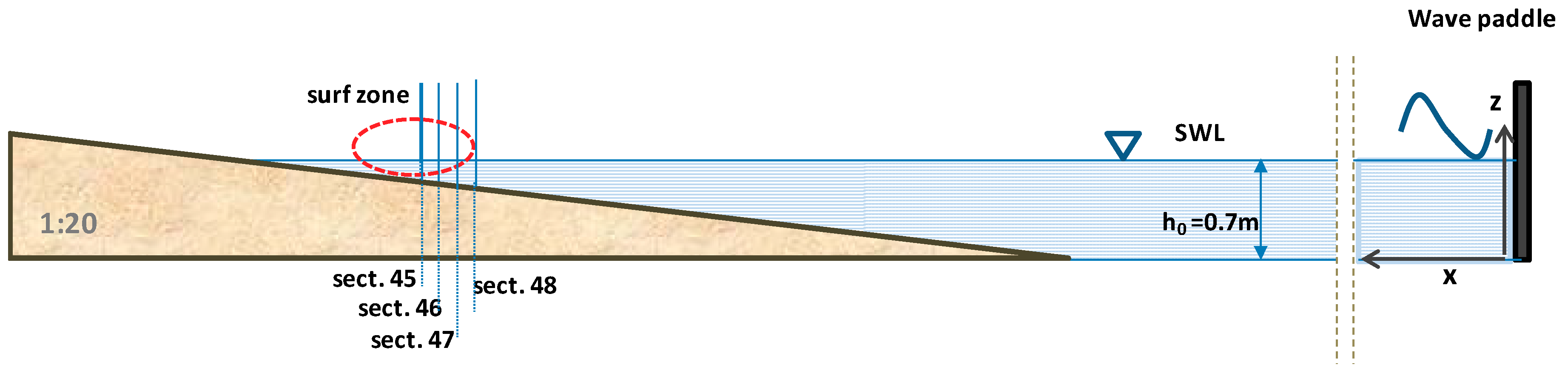
3.1. Phase-Averaged Distributions
To provide an insight in the flow field,
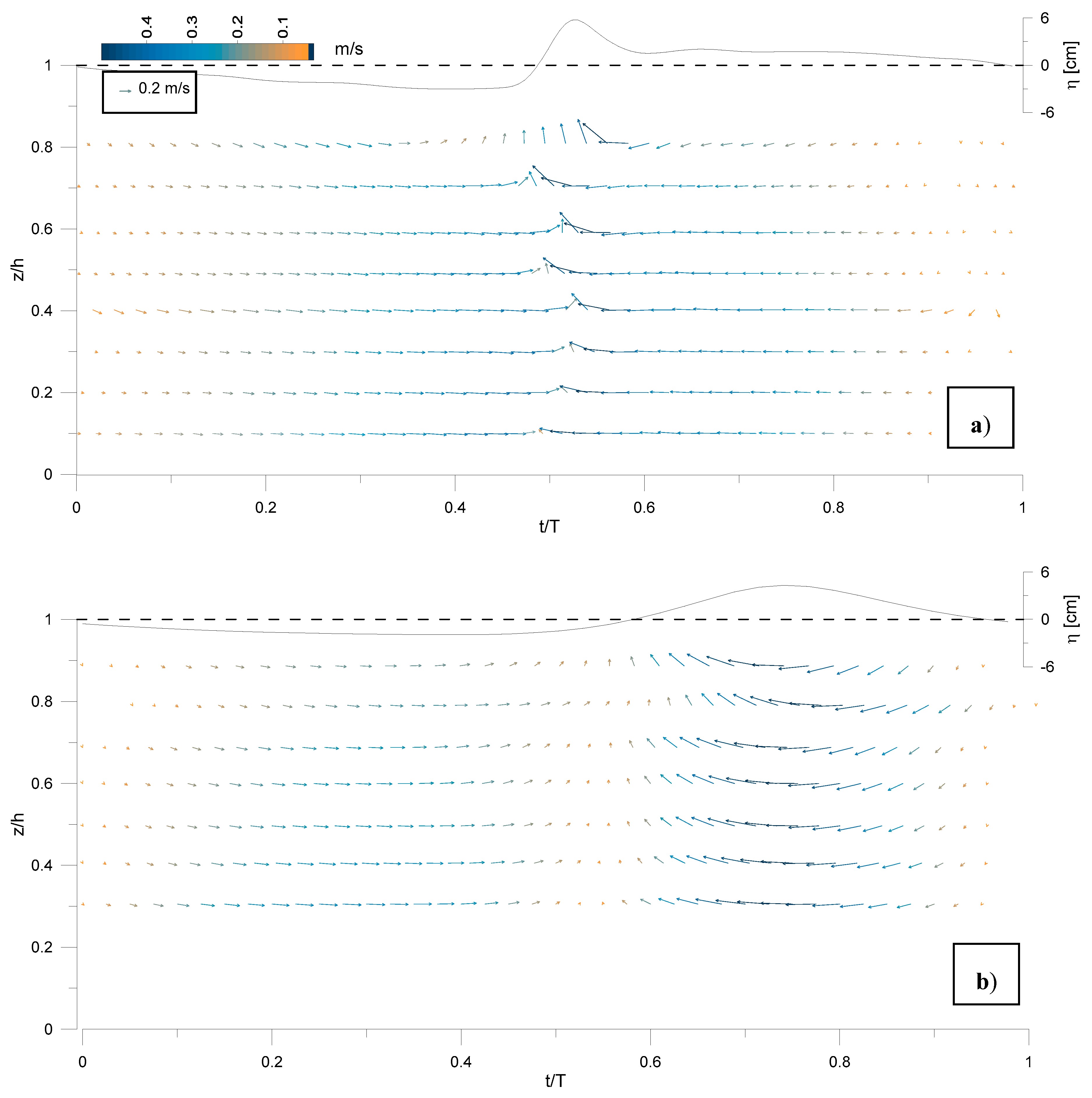
Figure 2 sketches the phase-averaged velocities (
uph,
wph) in a wave cycle, at the depths examined in Test_P (
Figure 2a) and Test_S (
Figure 2b) in section 47, i.e., where the breaking is incipient. The scale of the velocities is the same in both
Figure 2a,b. Since no noticeable deformation of the wave shape is observed through propagation over a distance of one wavelength, at least offshore the measuring section, the horizontal axis in
Figure 2 (showing the instant time in the period) may be regarded approximately as the horizontal spatial coordinate in the wavelength [
7,
15].
In the upper part of each plot is also added the phase-averaged elevation
η. A difference is immediately noticed in the vertical asymmetry of the incipient breaking wave between the two tests. As expected, in Test_P the wave crest is higher while the wave trough is lower than in Test_S. Moreover, the horizontal asymmetry highlights that in Test_P, the steep plunging breaker occupies a much more limited portion of the wavelength, compared to the case of the spilling breaker. Nevertheless, the distribution along the wave cycle of the phase-averaged velocities, plotted in
Figure 2 as vectors with components (
uph,
wph), is quite similar for Test_P and Test_S. Indeed, it resembles the wave elevation trend in both tests, with increasing velocities in the transition trough-crest (ascending phase) and decreasing velocities in the transition crest-trough (descending phase), at all depths. As well, a rotation of the velocity vectors is observed in the wave cycle at all depths, for both tests, coherently with the curvature of the surface, as already noted in previous experiments [
7,
31]. Consequently, during the first descending phase, the velocities are fairly uniformly oriented downwards and offshore, while in the accelerating phase, they rotate upward and onshore. In the plunging wave (
Figure 2a) below the wave crest, the maximum velocity value is noted, which is quite vertical in the most superficial layer. In the spilling case (
Figure 2b), below the crest, onshore horizontal velocity is observed at all depths. The reduction in the velocity values (absolute values) from the surface to the bottom is more marked in Test_P (
Figure 2a) than in Test_S (
Figure 2b).
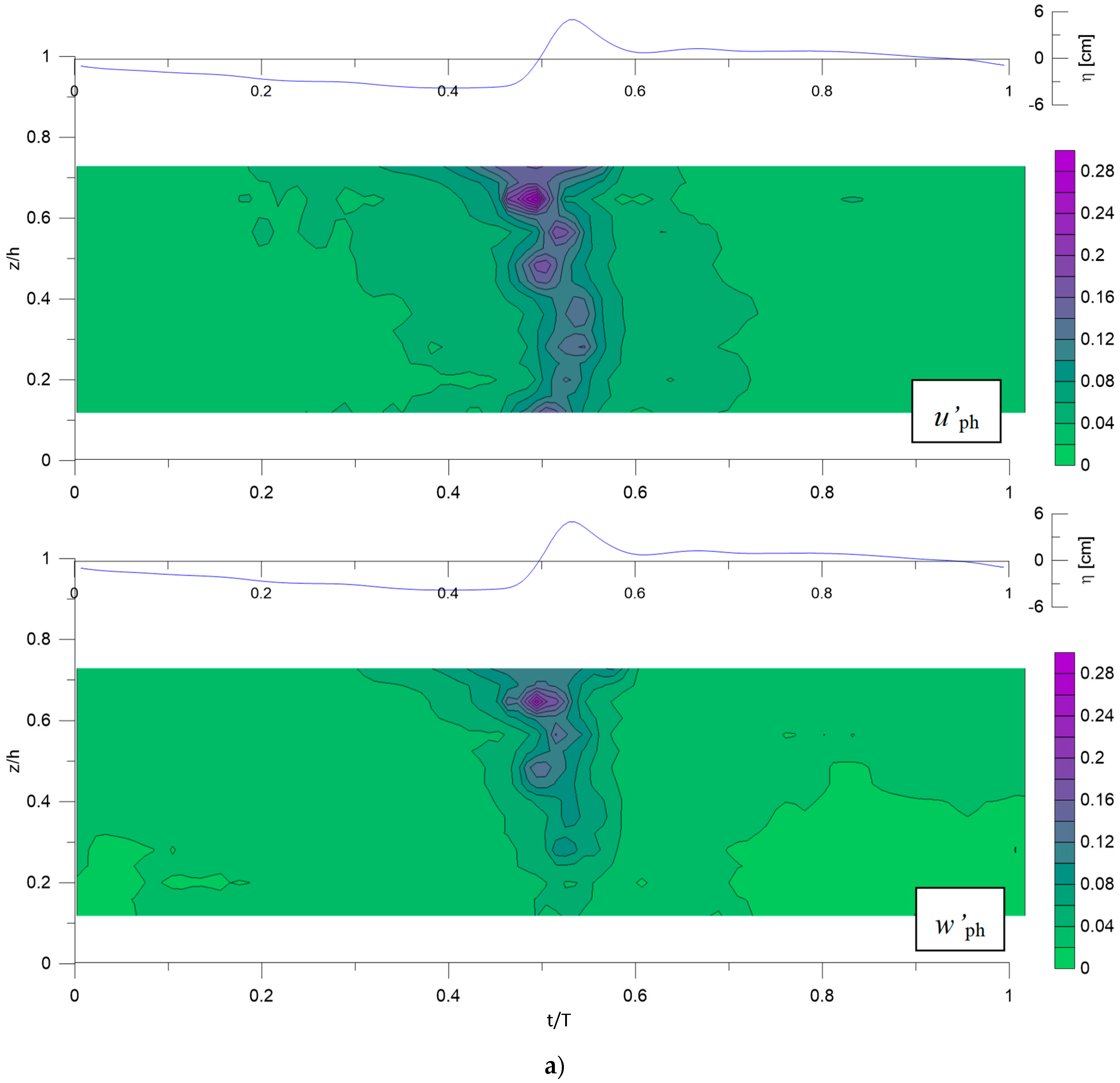
Referring to the same section 47, it is worth depicting the distribution in the wave cycle of the turbulence intensities
u’
ph and
w’
ph, computed by definition as the square root of (
u’
2)
ph and (
w’
2)
ph.
Figure 3a provides the turbulence intensities for Test_P, showing that the horizontal ones are higher than the vertical ones, as well as their decrease from surface to bottom, consistently with the incipient breaking. They both have their peak at the lower edge of the eddy region, also in accordance with Nadaoka et al. [
15]. Moreover, the tail of the contour lines is slightly oriented downwards and offshore, thus endorsing the possible presence of obliquely descending eddies (ODEs) numerically and experimentally proved by Lubin [
10,
24].
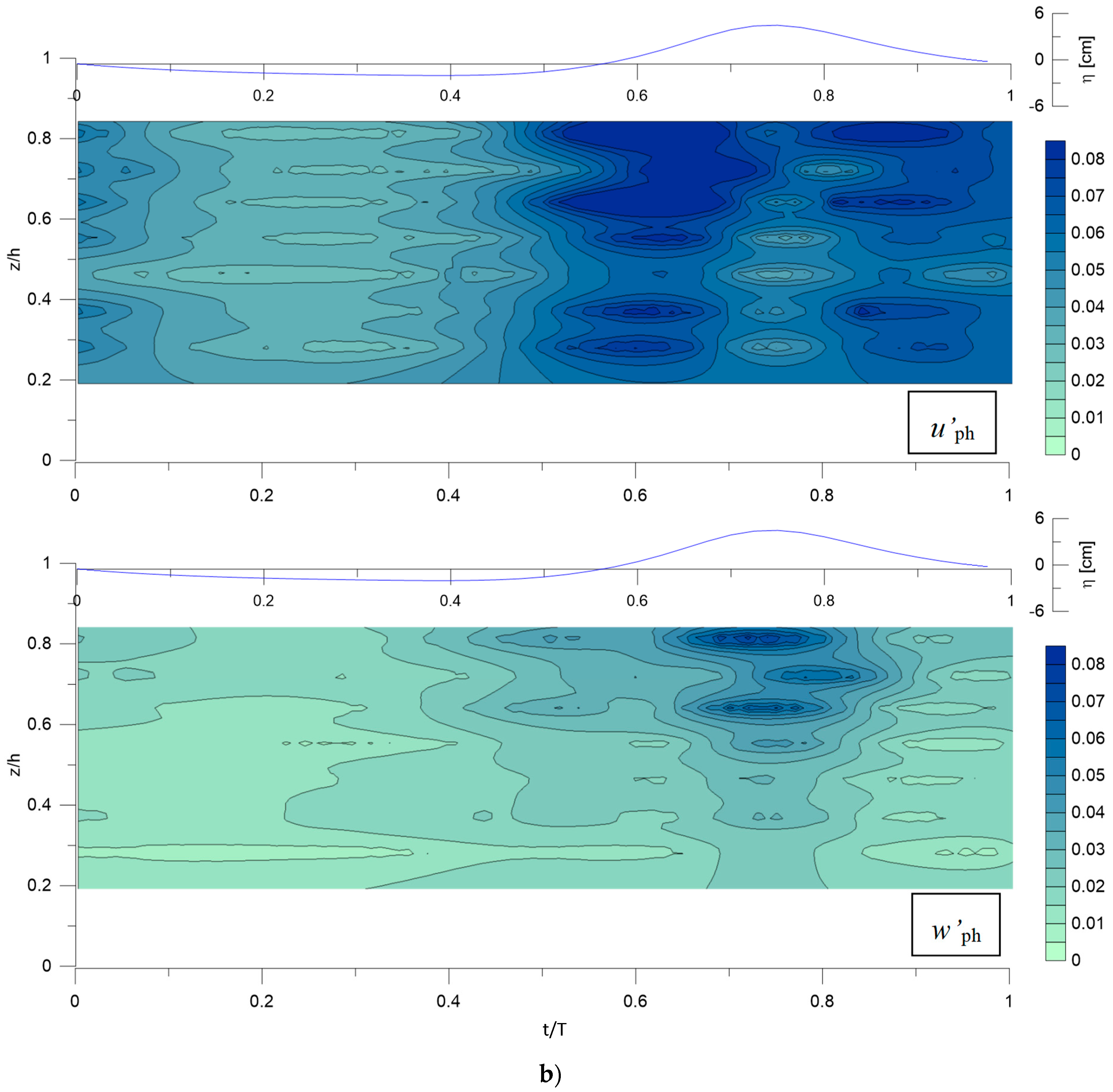
Figure 3b displays
u’
ph and
w’
ph values for Test_S, highlighting that in the spilling case they are approximately one third of those measured in Test_P. Furthermore, in this case, the
u’
ph values are greater than the
w’
ph values and they both reduce towards the bottom. The highest values for
u’
ph are localized under the ascending and descending phases of the wave, while the highest values for
w’
ph are localized under the crest. These patterns seem consistent with the propagating spilling bore. It is worth noting the recursive occurrence for both the tests of the turbulence intensities along the wave phases, thus stating an organized turbulent structure, which is quite typical for plunging and spilling waves.
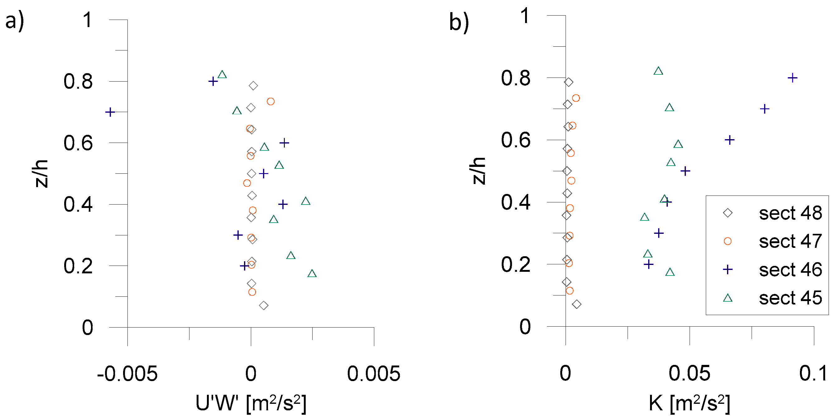
3.2. Time-Averaged Profiles
The vertical profiles of the time-averaged turbulent Reynolds shear stresses
U’
W’ and of the turbulent kinetic energy
K are examined in sections 48, 47, 46 and 45. For Test_P, they are respectively shown in
Figure 4a,b, where the plotted points refer to the locations below the still water level.
The turbulent Reynolds stresses
U’
W’ in
Figure 4a are quite negligible for sections 48 and 47, excepting the lowest point of section 48, in the boundary layer streaming, where the
U’
W’ value is positive, coherently with the effect of the bottom boundary layer. Referring in particular to section 47, the small order of magnitude of the
U’
W’ stresses (
Figure 4a) can be compared with the higher one of the
u’
ph and
w’
ph shown in
Figure 3a. It can be deduced that the major contribution to the total turbulent Reynolds stress in the incipient breaking (section 47) is essentially due to the phase-averaged turbulent velocities.
In section 46, immediately after the breaking, the
U’
W’ stresses are negative near the surface, and almost zero in the underlying region. In section 45 where the wave is reforming, they assume negative values near the surface and the highest positive values in the intermediate and lower part. This vertical gradient of
U’
W’ suggests a downward transport of turbulence from the surface, due to the occurred plunger [
3,
28], which is more evident in the upper region, for
z/
h > 0.4 in both sections 46 and 45. The largest positive
U’
W’ stresses are present in section 45, when the wave has formed again, near the bottom, proving that the effects of the bottom boundary layer are again felt [
3,
28,
31].
The different behavior between the prebreaking/incipient breaking sections (sections 48 and 47) and the sections shoreward the breaking (sections 46 and 45) is also evident in the vertical trends of the time-averaged turbulent kinetic energy
K, here computed following Svendsen [
32]. In fact, it tends to zero in sections 48 and 47 (
Figure 4b), while its highest values are assessed in section 46, especially for
z/
h > 0.5 due to the reversed plunger, where a decreasing trend towards the bottom is noted, meaning a spreading downward as in [
1]. Analogously, also in section 45, the
K profile has a similar shape, but the surface values are lower than in section 46, considering that the turbulence is decreasing with the increasing distance from the plunging breaker, meaning spreading downstream, in accordance with [
1].
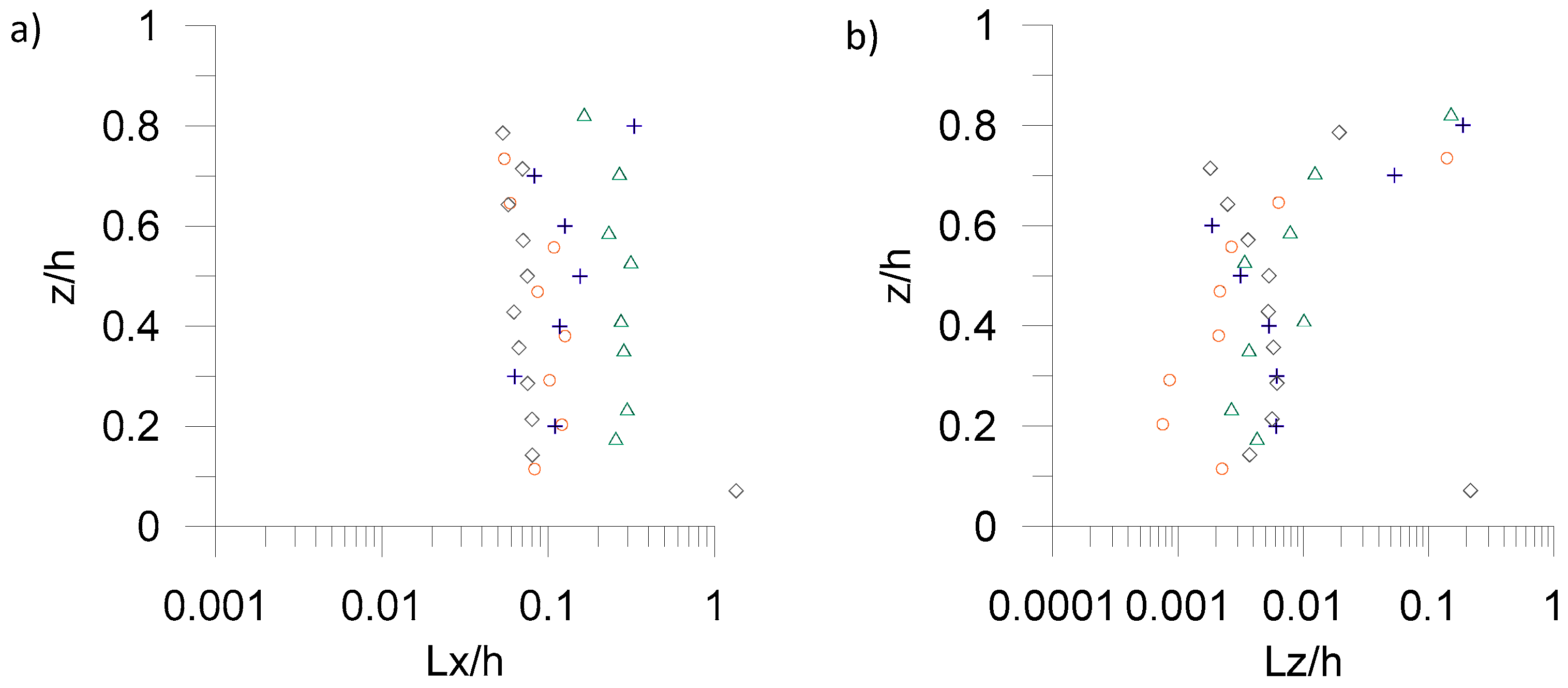
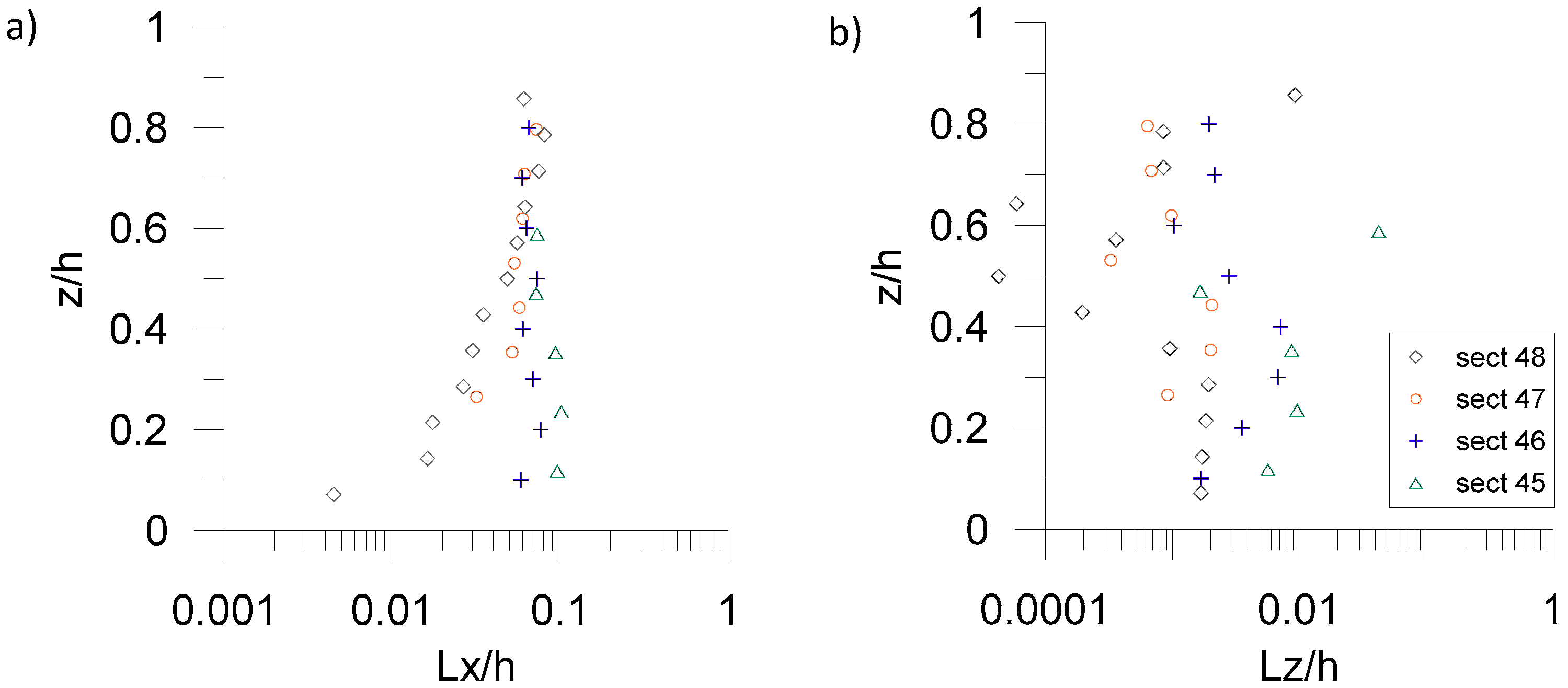
These observations are consistent for Test_P with the vertical distributions of the time-averaged integral length scales,
Lx and
Lz, associated with the turbulent large eddies (
Figure 5a,b) respectively in
x and
z directions. The integral and turbulent length scales have been computed by multiplying the local time-averaged velocity respectively for the turbulent time scale and the integral time scale. In turn, both turbulent and the integral time scales have been estimated based on the temporal autocorrelation function of the turbulent velocity fluctuations (for the detailed formulation, please refer to [
33]). It is noteworthy that the integral length scales
Lx, while having order O(0.1
h) in both sections 48 and 47 and 46, tend to be of order O(0.2 ÷ 0.3
h) in section. 45, thus proving that large eddies are stretched in the
x direction, as a consequence of the breaking.
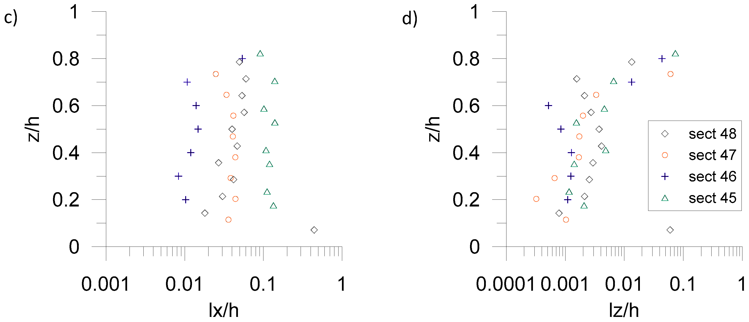
Moreover, by comparing
Figure 5a,c, it can be deduced that in sect. 46, immediately after the breaking, the
lx scales are one order lower than the
Lx scales. The same is also noted referring to the vertical
Lz and
lz scales (
Figure 5b,d), thus confirming the transfer of the energy contained at large scales to small scales, where it is turned into heat by viscosity [
7]. Moreover, for
z/
h > 0.6 both
Lz and
lz scales show increasing values as they approach the surface, with order ranging from O(0.01
h) up to O(0.1
h), consistently with the formation of the overturning plunging jet.
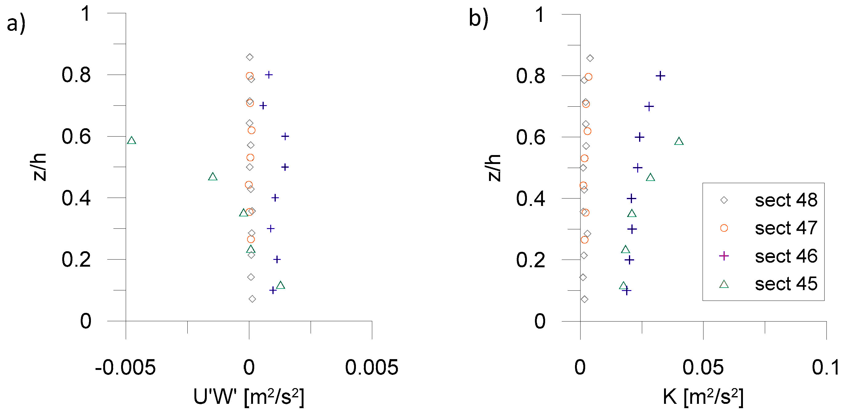
The same analysis of the time-averaged quantities has been performed also for Test_S. Analogously to Test_P, the
U’
W’ stresses are quite negligible in sections 48 and 47 (
Figure 6a). In section 46, when the spilling wave has just broken, there is a uniform positive trend along the
z-axis. Onshore, in section 45, the
U’
W’ profile shows the same bi-triangular shape already noted in Test_P (
Figure 4a), although in this case, lower positive values are displayed near the bottom and higher negative values for
z/
h > 0.3.
Furthermore, the distribution of
K (
Figure 6b) shows vertical trends already observed in Test_P, with decreasing values from the surface towards the bed in both sections 46 and 45. Nevertheless, in Test_S, the values of
K are halved with respect to Test_P. Moreover, the higher values of
K are observed in section 45, based on the presence of the bore after spilling, rather than in section 46. Comparing
Figure 6a,b with
Figure 4a,b, it can be assumed that with the bore propagating onshore, the spilling breaker continues to feed turbulence in the surface region, unlike the plunging wave, which produces higher turbulence but is located in a more compact area, where the breaking occurs. Moreover, the turbulent kinetic energy is less intense in the spilling case than in the plunging case.
Referring to the time-averaged integral length scales
Lx and
Lz (
Figure 7a,b), for each section there is a difference of approximately two orders of magnitude between them, proving the presence of eddies much more elongated in the horizontal direction than in the vertical direction. This horizontal stretching is thus greater for this spilling case than for the plunging one. Referring to the turbulent length scales
lx and
lz for Test_S, although they are lower than the corresponding integral ones,
lx has a comparable order of magnitude with
Lx and the same thing happens when comparing
lz and
Lz. Consequently, their graphs are not shown for brevity, being of little significance especially in the semi-logarithmic version. In any case, it is worth noting that despite eddies could not be observed directly, as for example in [
1,
17,
20,
22] based on PIV or V3V acquisitions, the distributions of these length scales permitted the indirect deduction of the presence of eddies in the target domain.
3.3. Quadrant Analysis
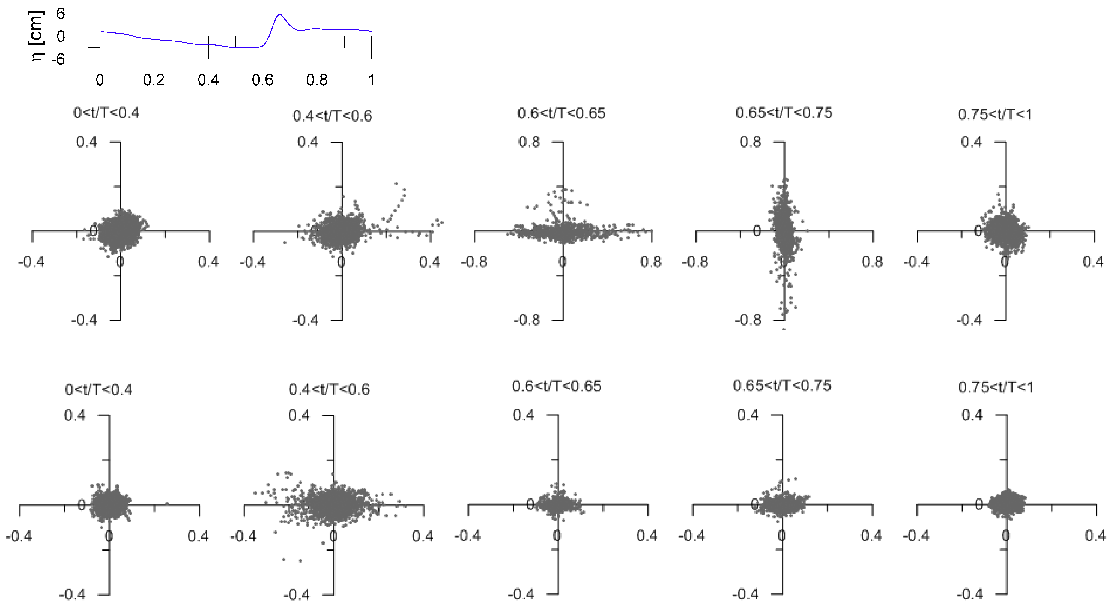
The results of the quadrant analysis are here described only referring to section 47, for the sake of brevity, for both Test_P (
Figure 8) and Test_S (
Figure 9).
Figure 8 and
Figure 9 display the quadrant plots of the instantaneous turbulent velocities (
u’,
w’) at five different phase intervals. The phases for which the data are plotted are written for each plot and have been selected based on meaningful parts along the wave cycle. Namely, for Test_P (
Figure 8): 0 <
t/
T < 0.4 descending phase; 0.4 <
t/
T < 0.6 descending phase up to wave trough; 0.6 <
t/
T < 0.65 ascending phase up to wave crest; 0.65 <
t/
T < 0.75 steep descending phase; 0.75 <
t/
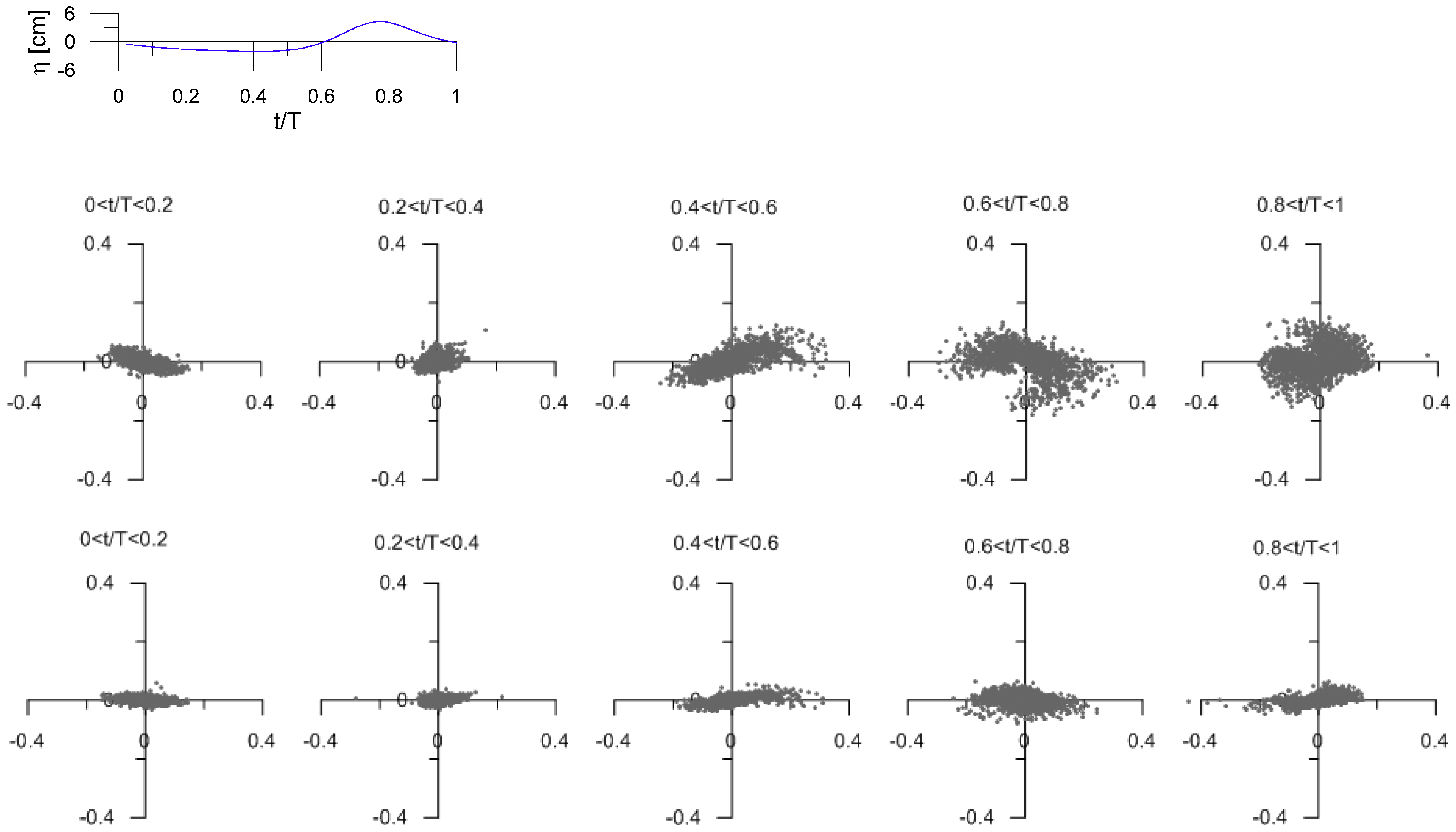
T < 1 flat descending phase. Analogously, for Test_S (
Figure 9): 0 <
t/
T < 0.2 descending phase; 0.2 <
t/
T < 0.4 flat descending up to wave trough; 0.4 <
t/
T < 0.6 gradual ascending phase; 0.6 <
t/
T < 0.8 ascending phase up to wave crest; 0.8 <
t/
T < 1 descending wave back. The phase-averaged wave elevation is also inserted in both figures to facilitate the identification of the abovementioned phase intervals. Further, the results in the top row refer to a near surface point, while those in the bottom row to a near bottom point. The scaling for the axes is the same for an easier comparison, except the interval 0.6–0.75 in Test_P (
Figure 8) due to high turbulent velocities.
The top row of
Figure 8 shows that in section 47 for the point at
z/
h = 0.7, the turbulent horizontal fluctuations
u’ are the largest during the ascending phase 0.6 <
t/
T < 0.65 (confirming [
29]) and under the wave crest
t/
T = 0.65. On the contrary, they are minimal in the descending phase (0.65 <
t/
T < 0.75), where the turbulent vertical fluctuations
w’ prevail and are the largest. In the remaining wave cycle, i.e., for 0 <
t/
T < 0.6 and 0.75 <
t/
T < 1, the plots tend to assume a quite circular shape, meaning that the (
u’
w’) points are fairly evenly distributed in all the quadrants Q1 ÷ Q4. For 0.4 <
t/
T < 0.6, the cloud of points is slightly elongated along the horizontal axis, thus the
u’ components prevail. For 0.75 <
t/
T < 1 the cloud of points is slightly aligned along Q2 and Q4 quadrants, proving the presence of ejections and sweep after the wave crest passage.
The bottom row of
Figure 8, referring to the point at
z/
h = 0.2 in section 47, depicts generally flattened plots. This is consistent with the presence of the bottom, reducing
w’ even if a large eddy due to wave breaking reaches the bottom boundary, as also noted in [
29]. The
u’ in 0.6 <
t/
T < 0.75 are much smaller than the corresponding ones near the surface, meaning that the passage of the wave crest has a negligible effect near the bottom. On the contrary, increasing values of
u’ near the bottom are noted rather than near the surface, during the descending phase and below the wave trough (0.4 <
t/
T < 0.6). From this analysis, a recursive tendency of the bursts in the wave cycle is evident, especially in the superficial layer, referring to the trough-crest transition and to the descending phase, under the back face of the wave.
The top row of
Figure 9 displays the quadrant analysis assessed for the spilling case (Test_S) in section 47, referring to the point at
z/
h = 0.7. In the descending phase 0<
t/
T < 0.2, the plot is sloped along Q2–Q4 quadrant, proving the presence of both ejections and sweeps. In the region approaching the trough (0.2 <
t/
T< 0.4), turbulent intensities reduce strongly, while they increase again during the ascending phase (0.4 <
t/
T < 0.6) where both outward and inward motions are noted (cloud deployed along Q1–Q3 quadrant). During the ascending phase up to the wave crest (0.6 <
t/
T < 0.8), the plot is directed along Q2–Q4, with the presence of ejections and sweeps, already noted in
Figure 3b. In the back face of the wave (0.8 <
t/
T < 1), again both the inward and outward motions are relevant (Q1–Q3).
Similar to the bottom row of
Figure 8, also in the bottom row of
Figure 9, referring to the point at
z/
h = 0.3, there are flattened clouds, which indicate the effect played by the bottom on the
w’ velocities. Furthermore, the largest
w’ values during the interval 0.6 <
t/
T < 0.8 are noted, when the crest is approaching. The largest
u’ values are observed in the transition trough-crest-trough (0.4 <
t/
T < 1). In the case of the spilling wave, the quadrant analysis highlights a dependence of the bursts on the wave phases even more marked with respect to the plunging case. Although different from the plunging case, in the spilling case, this effect is strongly noted close to the surface as well as close to the bottom.
Finally, the authors detected the coherent events, according to the method described in
Section 3.2. For both Test_P and Test_S, in each examined section, for three points (near surface, intermediate, near bottom), the assessed time series of
u’
w’ have been analyzed. The mean and the standard deviation were computed for each considered
u’
w’ signal and then the number of cases for which |
u’
w’| ≥ (μ + σ) were detected, thus identifying the coherent events in the series. The same has been made for detecting the most intense coherent events, for the condition |
u’
w’| ≥ (μ + 3σ) [
24].
Table 2 summarizes the results for the most significant sections, i.e., sections 47, 46 and 45. In the last two columns, the authors indicate: the percentage of coherent events %CE i.e., the number of data for which |
u’
w’| ≥ (μ + σ), rated by the total number of the acquired data, as well, the percentage of intense coherent events %IE, i.e., the number of data for which |
u’
w’| ≥ (μ + 3σ), rated by the total number of the acquired data.
For Test_P, the following can be noted. In section 47, the percentage of both coherent and intense coherent events increases from the surface towards the bottom. On the contrary, immediately after breaking in section 46, both percentages of coherent and intense coherent events, decrease with depth.
In section 45, the %CE percentage is the highest at the intermediate depth, while the %IE percentage remains quite unchanged at all depths. The comparison between sections 46 and 45 leads to thoughts of a spreading of the coherent events towards the bottom, while the intense ones are more localized in the upper layer, which is consistent with the splashed jet.
For Test_S, in section 47 the percentage of both coherent and intense coherent events decreased from the surface towards the bottom, being opposite to what was observed in Test_P in the same section, and presumably due to the formation of the roller. In section 46, the maximum %CE percentage is at mid-depth, while the %IE percentage tends to increase with depth. In section 45, the %CE percentage increases towards the bottom, while the %IE percentage decreases towards the bottom. It could be argued from the comparison of percentages in section 47 and 46 that in this case, the coherent and intense coherent events, initially more localized around the spiller, are spread downwards and onshore, thus affecting also section 45. The percentages computed are comparable with previous results [
23,
30].
Finally, it is observed that in Test_P, coherent and intense coherent events are more infrequent, especially referring to sections 46 and 45, where the percentages for Test_S are 2–3 times higher than in Test_P. This could be explained by the different breaking mechanism and the different nature of generated turbulence that characterize the two waves, especially considering the non-deterministic nature of a splashing jet.


