On the Dynamics of Canyon–Flow Interactions

Abstract

This paper explores the dynamical origin and physical characteristics of flow disturbances induced by ocean currents in interaction with shelf-incised submarine canyons. To this end, a process-oriented hydrodynamic model is applied in a series of case studies. The focus of studies is the canyon-upwelling process in which seawater is moved from the upper continental slope onto the shelf within a shelf-break canyon. Results reveal that the generation of canyon upwelling, to zero-order approximation, is a barotropic and friction-independent quasi-geostrophic process. Hence, the principle of conservation of potential vorticity for such flows is sufficient to explain the fundamental physical properties of the canyon-upwelling process. For instance, this principle explains the direction-dependence of the canyon-upwelling process. This principle also explains the formation of stationary topographic Rossby waves downstream from the canyon that can lead to far-field effects. Density effects, being of secondary influence to the canyon-upwelling process, result in the intensification of canyon-upwelling flows via the formation of narrow near-bottom density fronts and associated baroclinic geostrophic frontal flows. Findings of this work reveal that the apparently complex canyon-upwelling process is much more basic than previously thought.

1. Introduction

Submarine canyons are typical bathymetric features of continental margins of the oceans. They are often only a few hundred meters deep on a width of a few tens of kilometers. Submarine canyons cutting across the shelf break, so-called shelf-break canyons, are of particular importance to cross-shelf exchange processes in the oceans. Such canyons are not only important downslope conduits of dense shelf water (e.g., [1]) and turbidity currents (e.g., [2]). Under certain conditions shelf-break canyons also support the localized up-canyon flow of denser slope water across the shelf break and onto the continental shelf (e.g., [3]), hereafter referred to as canyon upwelling.

Some canyons, such as those located off the coasts of Washington State and British Columbia, are characterized by sidewalls of extremely steep slopes of up to 45° [4]. In other regions, such as the continental margin of southern Australia, shelf-break canyons are typically much less pronounced bathymetric features (see [5]), with sidewalls of milder bottom slopes <1°. The latter class of (probably more common) milder shelf-break canyons is the subject of this work.

One of the most essential conditions for the canyon-upwelling process is the presence of ambient ocean currents flowing against the propagation direction of free coastal Kelvin waves (or continental shelf waves) (e.g., [6]). Surprisingly, the theoretical understanding of this fundamental direction-dependency of the canyon-upwelling process is still incomplete. Previous theoretical studies on the canyon-upwelling process indicate an extremely high dynamical complexity characterized by many topographic and dynamical scales and associated non-dimensional numbers. For instance, Allen and Hickey’s study [4] was based on 11 scales and nine non-dimensional numbers.

Is such a high level of complexity really required to capture and describe the fundamental dynamics of the canyon-upwelling process? Some previous studies indicate that, under typical circumstances, certain scales are less relevant, or even irrelevant for the canyon-upwelling process including canyon width, canyon length, bottom friction, and density stratification above shelf-break depth [7,8]. Findings [8] even suggest that the local density stratification at canyon depth is of secondary importance to the process. Could it be that, perhaps, the canyon-upwelling process is much more basic and less complex than previously thought?

It is worth mentioning that the radius of curvature ℜ of isobaths at the upstream side of the canyon’s head appeared as a central scale in the canyon research of recent years (e.g., [4]). This radius measures the curvature of the outer flanks of the canyon, not that within the canyon. While this scale has been shown to control the behavior of buoyancy-driven flow traveling over a canyon [9], its relevance to the canyon-upwelling process has not been verified so far.

The principal research objective of this study was to reveal the fundamentals of the dynamics involved in the upwelling in a shelf-break canyon. Scientific questions addressed in this study were fairly basic: Is the canyon-upwelling process initiated by barotropic or baroclinic disturbances? Which of the many scales involved in the process are relevant? Why is the canyon-upwelling process dependent on the direction of the ambient flow?

This paper is organized as follows. Section 2 outlines the methodology employed in this work. Findings are presented and discussed in Section 3. Section 4 closes with a summary and conclusions.

2. Materials and Methods

This study employs the three-dimensional COHERENS model [10], which is based on terrain-following sigma coordinates. The model settings used are similar to those of previous studies [5,11]. The model domain (Figure 1) is 240 km in length and 120 km in width resolved by a horizontal grid spacing of 1 km and 20 vertical sigma levels. The idealized continental margin consists of a straight coastline, a continental shelf, a continental slope, and a single shelf-break canyon.

The continental shelf of the control experiment has a width of 60 km and a depth ranging from 100 m at the coast to 200 m at the shelf-break. The associated angle is 0.1° corresponding to an inclination of s = 0.0017 or 1.7 m/km. The continental slope has an angle of 0.46° (inclination is 8 m/km). Maximum water depth is cut off at 600 m to maximize model efficiency. Variations of this cut-off depth had no noticeable impact on the results (not shown). It should be noted that the deepest portions of the continental slope are smoothed such that the seafloor is plane along the open offshore boundary.

Sensitivity experiments address variations of shelf-break depth and inclination of the continental shelf (Figure 2). To this end, the shelf-break depth, h_o, is varied between 150 m and 250 m, and bottom inclinations, s, of the shelf between 0.83 m/km and 3 m/km. As far as the author is aware, variations of s (which turns out to be a central scale) have not been considered in previous studies.

The idealized submarine shelf-break canyon has a width of W ≈ 30 km and a maximum depth relative to the ambient seafloor of Δh = 100 m. Canyon walls attain a maximum slope of 0.26° (inclination is 4.5 m/km). In the basic configuration, the radius of curvature of isobaths at the upstream side of the canyon’s head is ℜ ≈ 20 km. This canyon configuration was created via application of the diffusion equation to a coarse block-type canyon prototype.

In addition, various canyon shapes with different radii of curvature ℜ were tested to verify the role that this scale plays in the canyon-upwelling process. Here, only results of the most extreme case of a box-type canyon are discussed (Figure 3). Although this configuration resembles a canyon of vertical sidewalls, the slope of the sidewalls is constrained by the ratio between canyon depth and horizontal grid spacing. The choice of a horizontal grid spacing of 1 km, as used in this study, produces an inclination angle of the canyon’s sidewalls of ~6°. This test case corresponds to ℜ ≈ 1 km, i.e., 20 times smaller than in the control experiment.

With the use of 20 equidistant sigma levels, the vertical grid spacing increases to a maximum of 30 m in the deepest portions of the model domain. This is sufficiently fine to capture the integral effect of bottom Ekman-layer dynamics (which turn out to be irrelevant to the canyon-upwelling process). The model ocean has an initially linear vertical density stratification characterized by a stability frequency of N = 3.25 × 10⁻³ s⁻¹. This corresponds to a realistic maximum internal wave period of 32 min. The Coriolis parameter was set to f = ±1 × 10⁻⁴ s⁻¹, representing mid-latitudes of either the northern or the southern hemisphere. The Pacanowsky–Philander turbulence scheme [12] was adopted to calculate sub-grid scale vertical turbulent viscosity and diffusivity. This scheme is Richardson-number dependent. Bottom friction is calculated from a quadratic approach based on a uniform bottom roughness length of 5 mm. Horizontal eddy viscosity and diffusivity are set to a uniform value of 1 m²/s.

In the control experiment, the model is forced via gradual lowering (if f is negative) or raising (if f is positive) the coastal sea level η_o by 10 cm over the first five simulation days, keeping it at this constant level afterwards. The sea level along the deep-open boundary is kept at its initial value during the entire simulation. This method initiates a steady barotropic geostrophic flow being right-bounded by the coast in both the northern and southern hemisphere scenarios. Note that this method tends to make the coastline a streamline for geostrophic flow and eliminates the generation of fast-propagating (~30 m/s) coastal Kelvin waves that could lead to severe unwanted problems at open boundaries.

The geostrophic flow created by this method is not uniform in the offshore direction (Figure 4a). Instead, it varies in the offshore direction attaining a weak relative vorticity of ∂u/∂y ≈ 0.01|f|. The imposed initial squeeze/stretching of the water column near the coast created this flow structure. Relative vorticity inherent with this ambient coastal flow is substantially weaker than that induced via canyon–flow interaction (see Section 3.2). In the control experiment, the speed of the ambient flow in vicinity of the shelf break is U ≈ 0.1 m/s. Sensitivity experiments considered ranges of U between 5 and 15 cm/s, which is realized through variation of the coastal sea-level forcing.

Figure 4b displays the maximum possible degree of water column stretching that the water column can experience when being moved straight across the canyon. This degree of stretching peaks at around 0.44 (or 44%) near the shelf break.

Passive Eulerian tracer is used to illustrate the evolution of density disturbances. Initially, this tracer field is laterally uniform and varies linearly between zero and unity over the maximum depth of the model domain. Both density and Eulerian tracer concentration are kept fixed at the upstream boundary. Otherwise, simple zero-gradient boundary conditions are used for all variables.

In addition, after the initial five-day adjustment period, neutrally buoyant Lagrangian floats are injected on the upper continental slope within a distance of 10 m from the seafloor. To this end, floats are released near the upstream boundary at a rate of 15 floats per 90 min, using a total of 3000 floats. This method, which commences after the initial five days of forcing adjustment, creates a continual stream of floats emerging from the upstream boundary at random locations over a period of 12.5 days. Note that steady-state dynamics establishes within 5–10 days of simulations, thus the resultant trajectory of a float is invariant on its release time. The large number of floats used is more than sufficient to resolve the spatial structure of the simulated flows (see Section 3.2). See [10] for technical details of the Lagrangian particle module.

Using the above configuration, two scenarios are considered. The first scenario explores right-bounded flow in the northern hemisphere (equivalent to left-bounded flow in the southern hemisphere) being characterized by free continental shelf waves travelling into the same direction as the coastal flow. This scenario is henceforth referred to as “topographic steering scenario”. The second scenario explores right-bounded flow in the southern hemisphere (equivalent to left-bounded flow in the northern hemisphere) being characterized by free continental shelf waves travelling opposite to the ambient coastal flow. This scenario is henceforth referred to as “canyon-upwelling scenario”. For comparison, both scenarios are repeated neglecting both density stratification and bottom friction. Note that both Klinck [13] and the author’s previous studies [7] considered similar comparisons, but with model domains too small to capture the development of topographic waves outside the canyon. The total simulation time of all experiments is 25 days, over which no dramatic disturbances develop near the open boundaries.

3. Results and Discussion

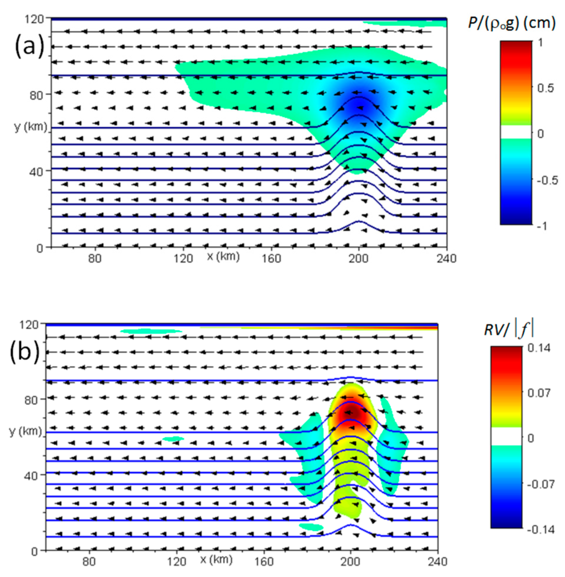
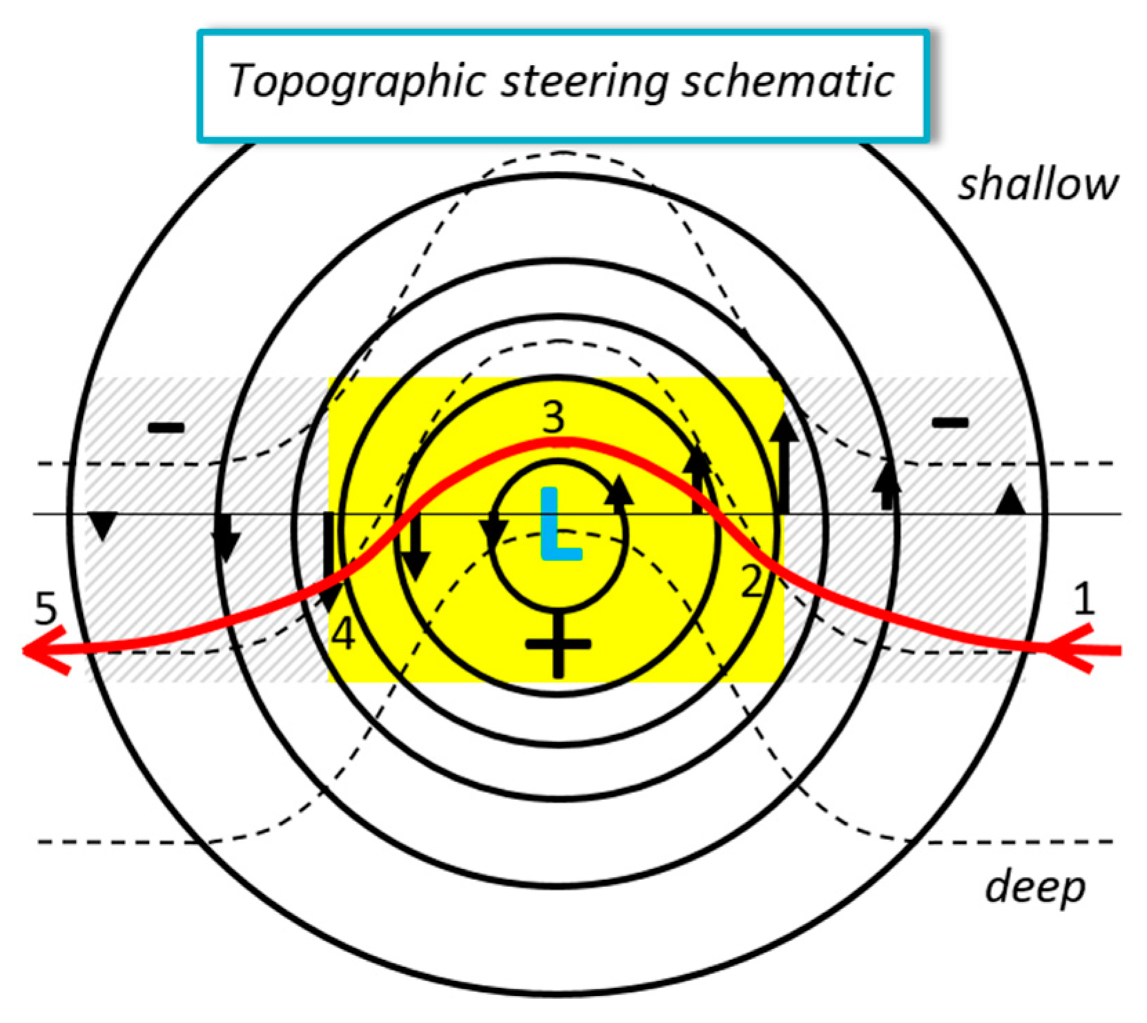
3.1. Topographic Steering Scenario

Right-bounded flow in the northern hemisphere is smoothly topographically steered across the shelf-break canyon (Figure 5). Note that the same applies to left-bounded flow in the southern hemisphere. Here, flow disturbances were created in interaction with the canyon and were carried downstream via topographic Rossby waves propagating into the same direction as the ambient flow. Flow–canyon interaction led to establishment of a low-pressure anomaly centered over the canyon head in which the sea level was lowered by ~0.8 cm (Figure 6a). Indeed, such small sea-level anomalies cannot be detected by satellite altimetry. In turn, this low-pressure anomaly created a quasi-geostrophic flow field of positive relative vorticity (∂v/∂x − ∂u/∂y > 0) (Figure 6b). The exclusion of density and frictional effects yielded identical results (not shown). Hence, flow disturbances created through interaction with the canyon obeyed the principle of conservation of potential vorticity along the streamlines of the barotropic flow; that is,

$$\frac{f+\partial v/\partial x-\partial u/\partial y}{h_o+\delta h}=const$$

(1)

where h_o is the initial thickness of the water column, and δh the change in thickness that this water column experiences along the trajectory of the flow. During the process, the alongshore flow of speed U, which varies on the scale of shelf width, Y, becomes converted into up-canyon flow of speed V confined to canyon width, W. Scaling arguments hence suggest that V/W >> U/Y, i.e., ∂v/∂x >> ∂u/∂y in Equation (1). If we further assume that relative velocity is negligibly small upstream from the canyon, Equation (1) can be reformulated as:

$$\frac{\partial v}{\partial x}\approx f\frac{\delta h}{h_o}$$

(2)

The key implication of Equation (2) for the topographic steering scenario is that positive relative vorticity (∂v/∂x > 0) over the canyon can only be accommodated if the flow remains slightly stretched (δh/h_o > 0) during its passage across the canyon. Hence, the water column moves into slightly deeper regions as it enters the canyon, while the quasi-geostrophic flow anomalies inside the canyon operate such that the flow trajectory attains the same curvature as underlying isobaths. To this end, while crossing the canyon, the water column stays relatively close to its initial thickness reference h_o. Note that this zone of positive relative vorticity is located between transition zones of weak negative relative vorticity (see Figure 6b), which result from the weakening of pressure anomalies outside the canyon. Figure 7 summarizes this dynamic behavior that characterizes the topographic-steering scenario.

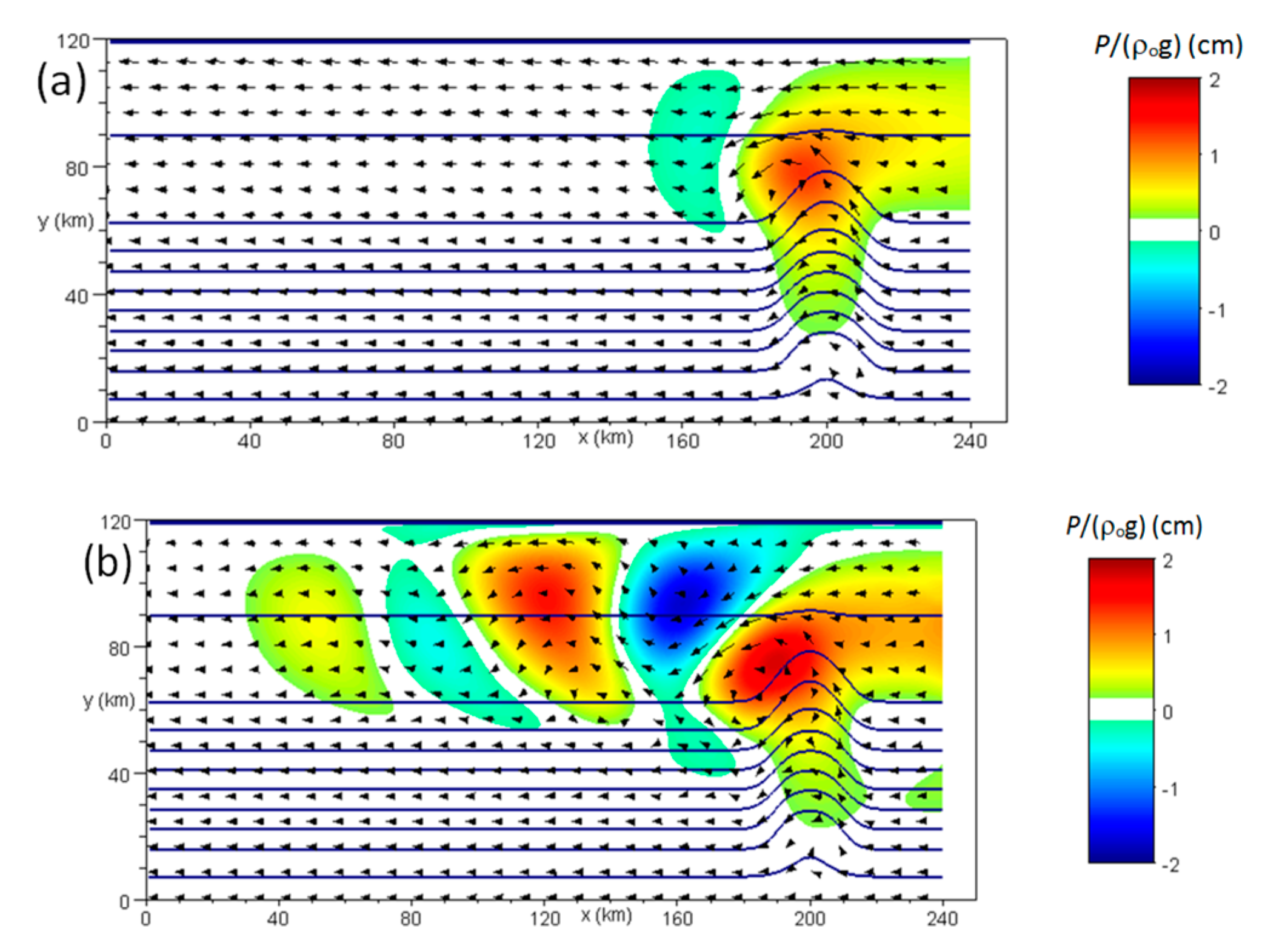
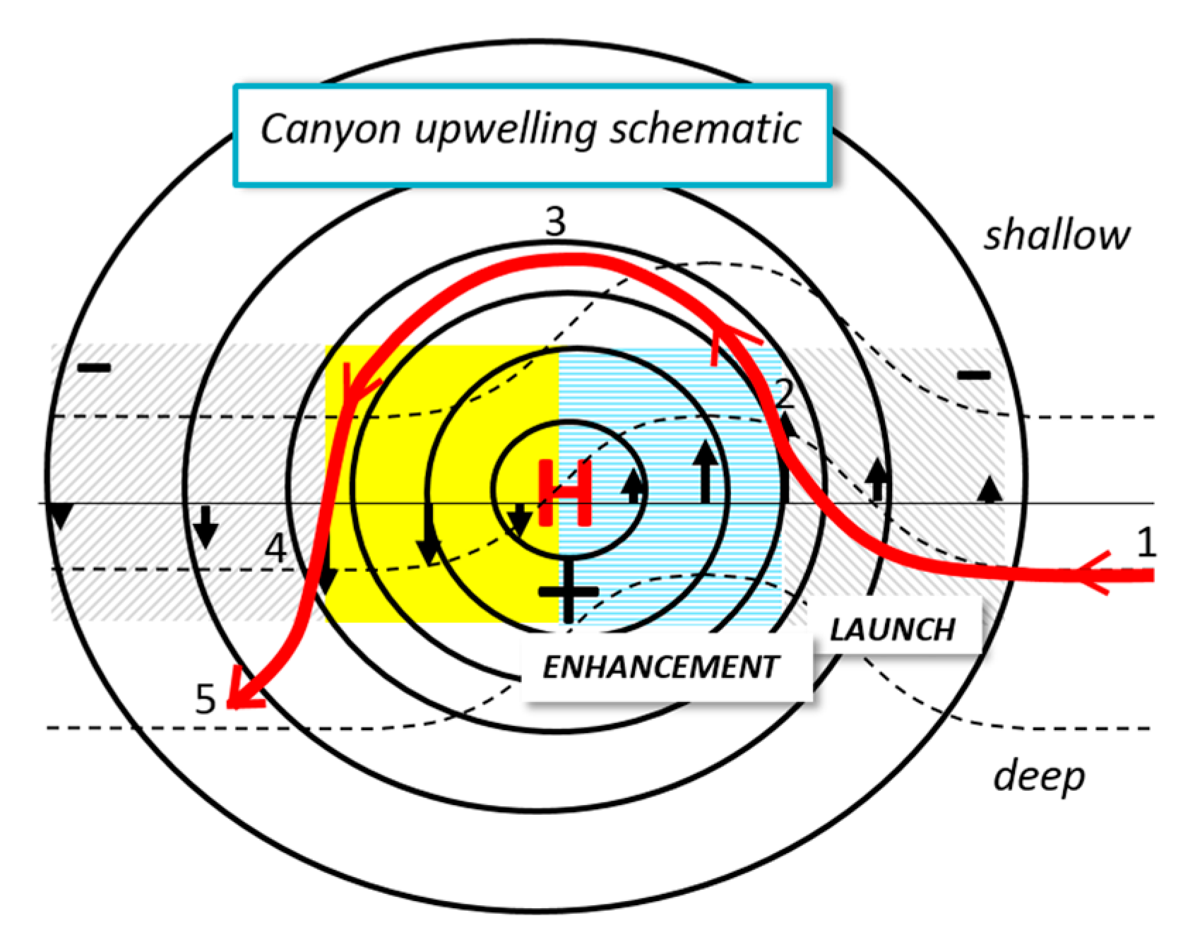
3.2. Canyon-Upwelling Scenario

The situation changes dramatically for right-bounded flow in the southern hemisphere (or, analogously, for left-bounded flow in the northern hemisphere). Here, flow–canyon interaction leads to localized up-canyon flow of deeper slope water across the shelf break and onto the continental shelf (Figure 8a). The speed of this up-canyon flow in the control experiment is ~12 cm/s. Simultaneously, a standing wave feature forms along the shelf break downstream from the canyon at a wavelength of ~65 km. Interestingly, the flow separates into two portions with a shallower branch forming part of the canyon upwelling and a deeper branch being largely unaffected by interactions with the canyon. Exclusion of density and frictional effects give similar flow trajectories near the canyon (Figure 8b). Again, this indicates that, to zero-order approximation, the interaction of coastal flows with a canyon can be accurately described by quasi-geostrophic theory for barotropic flows. See Section 3.3 for a discussion of baroclinic aspects of the canyon-upwelling process.

Flow–canyon interaction leads to the establishment of a high-pressure anomaly near the canyon head (Figure 9a), noting that the topographic steering scenario resulted in a low-pressure anomaly (see Figure 6a). More importantly, and in contrast to the latter scenario, the center of this pressure anomaly establishes slightly downstream from the canyon axis. Again, pressure anomalies are most pronounced near the canyon head, where the possible degree of water-column stretching is at maximum (see Figure 4b). Here, pressure anomalies correspond to a sea-level elevation of ~1.5 cm. In contrast to the topographic steering case, alternating high and low pressure zones develop downstream from the canyon on the continental shelf (Figure 9b). This pressure pattern is the signature of a stationary wave of a wavelength of ~90 km.

The canyon–flow interaction process created a relatively complex relative-vorticity field (Figure 10), which is discussed in the following. Figure 11 shows a schematic of this process, which can be classified as a failure of topographic steering.

A high-pressure anomaly in the southern hemisphere is associated with quasi-geostrophic flow anomalies of positive relative vorticity. Therefore, in contrast to the topographic-steering case, conservation of potential vorticity (Equation (2)) now implies that the water column has to be compressed (δh/h_o < 0) for the water column to be able to cross the shelf-break canyon. However, what initially happens as the flow enters the canyon (Phases 1 → 2 in Figure 11) is the opposite. Owing to inertia, the water column is subject to water-column stretching. This creates a narrow band of negative relative vorticity along the upstream (inflow) side of the canyon (Figure 10a,b, and Figure 12a). There is ample observational evidence of this water-column stretching in deeper portions of shelf-break canyons (see [4]). This narrow zone supports up-canyon flow of strong lateral velocity shear. It operates as a “launch zone”, moving the water column across its native isobath into shallower water, where it is eventually exposed to the required water-column compression (Phases 2 → 3 in Figure 11). Note that the maximum speed of up-canyon flow coincides with this crossing location.

Before the water column can return to deeper water, it is still subjected to up-canyon flow until it passes the center of the high-pressure anomaly. Hence, adjacent to the launch zone is an enhancement zone in which the water column is moved farther away from its reference thickness h_o. This enhancement zone initiates a positive relative-vorticity anomaly outside the canyon, which is the starting point for the development of a stationary topographic Rossby wave in the lee of the canyon (Figure 9b and Figure 12b; Phases 4 → 5 in Figure 11). This anomaly is most pronounced near the shelf break, which is the region of the largest maximum possible water-column stretching (Figure 2b).

Another interesting feature seen in the model prediction is that the positive dynamic pressure anomaly initiates a branch of flow that is geostrophically steered back towards the canyon (Figure 9a,b). Such return flows are the signature of a breaking topographic Rossby wave, as illustrated in Figure 12c. This wave breaking, which was also evident from the float trajectories (Figure 8a,b) explains the creation of zones of negative relative vorticity in adjacent deeper water (see Figure 10a,b).

According to linear theory, the phase speed of barotropic topographic Rossby waves along isobaths is given by [14]:

$$c=\frac{sg}{f}\frac{1}{1+{\left(2\mathsf{\pi }R/L\right)}^2}$$

(3)

where s is bottom inclination of the seafloor, L is wavelength, and R = (gh_o)^0.5/|f| is the barotropic Rossby radius of deformation (h_o is ambient total water depth). Note that free topographic Rossby waves travel with shallower water on their right (left) in the northern (southern) hemisphere. A standing wave occurs if the ambient flow eliminates the wave propagation such that the wave is kept stationary in space. This happens for a Froude number of unity (Fr = |U/c| = 1), yielding:

$$U=\frac{sg}{f}\frac{1}{1+{\left(2\mathsf{\pi }R/L\right)}^2}$$

(4)

Hence, the matching condition in Equation (4) determines the wavelength L of the resultant standing wave, given by:

$$L=\frac{2\mathsf{\pi }R}{\sqrt{sg/\left(fU\right)-1}}$$

(5)

For relatively short waves (L << R), which is the case here, Equation (5) can be further simplified to:

$$L\approx 2\mathsf{\pi }R\sqrt{fU/\left(sg\right)}=2\mathsf{\pi }\sqrt{U{h}_o/\left(sf\right)}$$

(6)

To test Equation (6), sensitively experiments considered U between 5 and 15 cm/s; shelf-break depths, h_o, between 150 m and 250 m; and bottom inclinations, s, of the shelf between 0.83 and 3 m/km. Overall, the predicted wavelength of pressure disturbances forming downstream from the canyon are in excellent agreement with the theoretical values (Figure 13). Geometric scales of the shelf-break canyon itself (e.g., canyon width and depth) did not significantly modify this wavelength (results not shown).

It should be highlighted that the canyon–flow interaction creates a high-pressure anomaly near the head of the canyon and a pressure gradient that, overall, is directed from shallower to deeper water (Figure 9). This offshore gradient, also identified in my previous work [7], conflicts with claims by other canyon researchers who suggested that canyon upwelling was caused by onshore pressure gradients [4,6,15]. Here, this conflict is eventually resolved with the demonstration that the canyon-upwelling flow is a quasi-geostrophic flow being exclusively driven by cross-canyon and not along-canyon pressure gradients.

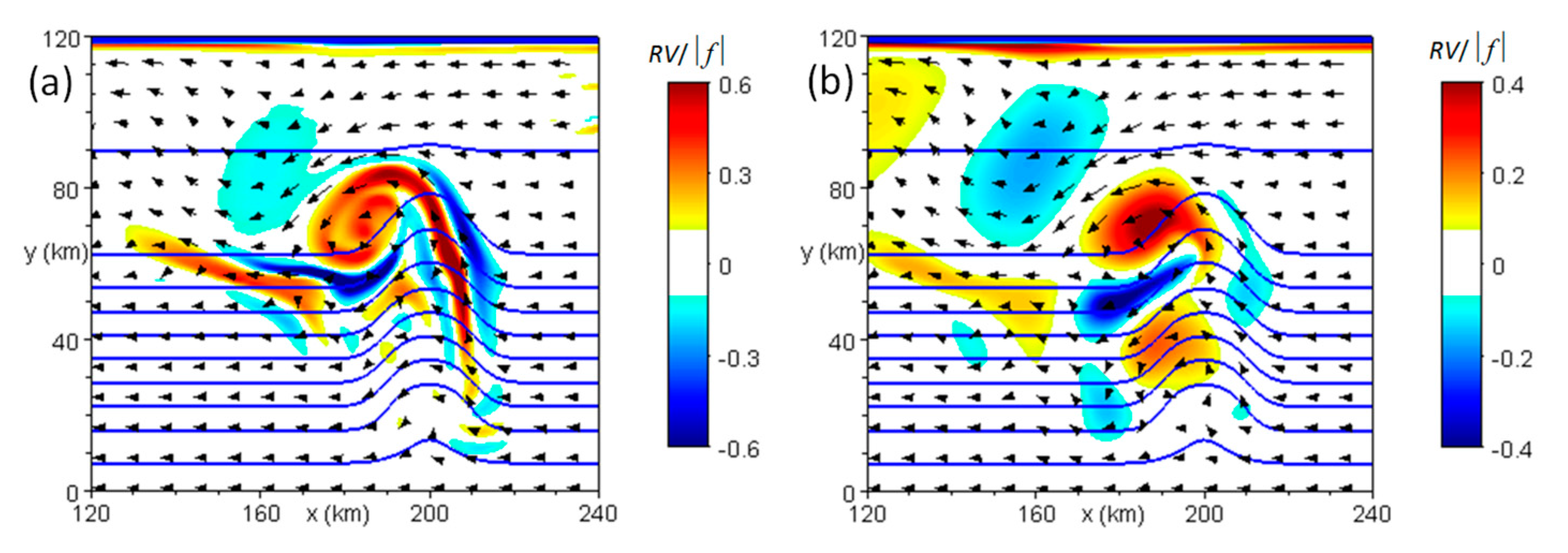
3.3. Impacts of Density Effects

In the barotropic case, water-column stretching/compression triggered relative vorticity values of magnitude being close to the maximum possible value of δh/h_o|f| = 0.44|f| (see Figure 4b and Figure 10b). In the presence of density stratification, the magnitude of relative vorticity even exceeded this barotropic limit (see Figure 10a). Hence, although not essential in the generation of canyon upwelling, density stratification clearly enhances canyon-upwelling flows. This is in agreement with previous estimates of canyon-upwelling fluxes [8]. This enhancement occurs via baroclinic geostrophic adjustment and leads to the formation of narrow (few kilometers wide), near-bottom density fronts of enhanced quasi-geostrophic flows (Figure 14). These flows are characterized by small pressure anomalies of the order of only 0.8 cm (expressed as equivalent sea-level elevation). Nevertheless, given the small (~few km) width of these fronts, the associated pressure gradients still results in a substantial enhancement of up-canyon flows by ~5 cm/s. In comparison to the barotropic case, this enhancement triggers a clearer separation between the upwelling branch of the flow and the deeper flows, which are little impacted during their interaction with the canyon (compare Figure 8a,b) as the maximum possible amount of water-column stretching decreases in deep water (Figure 2b).

Overall, there appear to be three different pressure and length scales involved in the process. First, the ambient barotropic geostrophic flow is characterized by a pressure equivalent of ~10 cm in sea surface elevation over the width of the shelf (~60 km) (Figure 14a). Second, the stationary topographic Rossby waves is characterized by a pressure equivalent of ~2 cm in sea surface elevation over the wavelength of this wave (~60 km) (Figure 14b). Third, baroclinic near-bottom jets are characterized by a pressure equivalent of <1 cm on frontal widths of ~1 km (Figure 14c).

3.4. Confinement of Canyon Upwelling to the Upper Continental Slope

The float trajectories of the control experiment indicate that the canyon-upwelling process is confined to the upper portion of the continental slope (see Figure 8a). Several factors are responsible for this feature. First, the greatest vorticity disturbance occurs near the shelf break where the initial water-column stretching is maximal. Second, this initial stretching vorticity triggers the creation of a localized high-pressure center near the head of the canyon (Figure 9). Strong cross-isobath flow disturbances are only supported in close vicinity of this center near the shelf break, but not in deeper portions of the canyon where pressure anomalies are substantially weaker. Third, whereas pressure anomalies peak slightly downstream from the canyon axis on the upper continental slope, they are more aligned with the canyon axis in deeper portions of the canyon (Figure 9). This closer alignment operates in support of the topographic-steering process in deeper portions of the canyon.

3.5. Impacts of Radius of Curvature

The shelf-break canyon of the control experiment was characterized by a radius of curvature of isobaths at the upstream side of the canyon’s head of ℜ = 20 km. In contrast, this radius was reduced to ℜ = 1 km when using a block-type canyon prototype (see Figure 3). Interestingly, this substantial difference in canyon shape had remarkably little impact on the canyon-upwelling process (Figure 15). Both the wavelength of stationary topographic Rossby waves and density anomalies formed on the continental shelf were largely unaffected. This indicates that the role of ℜ in the canyon-upwelling process may have been overestimated in previous studies.

4. Conclusions

The method of process-oriented high-resolution hydrodynamic modeling was employed to study the interaction of coastal flow with a shelf-break canyon. The key findings of this study can be summarized as follows:

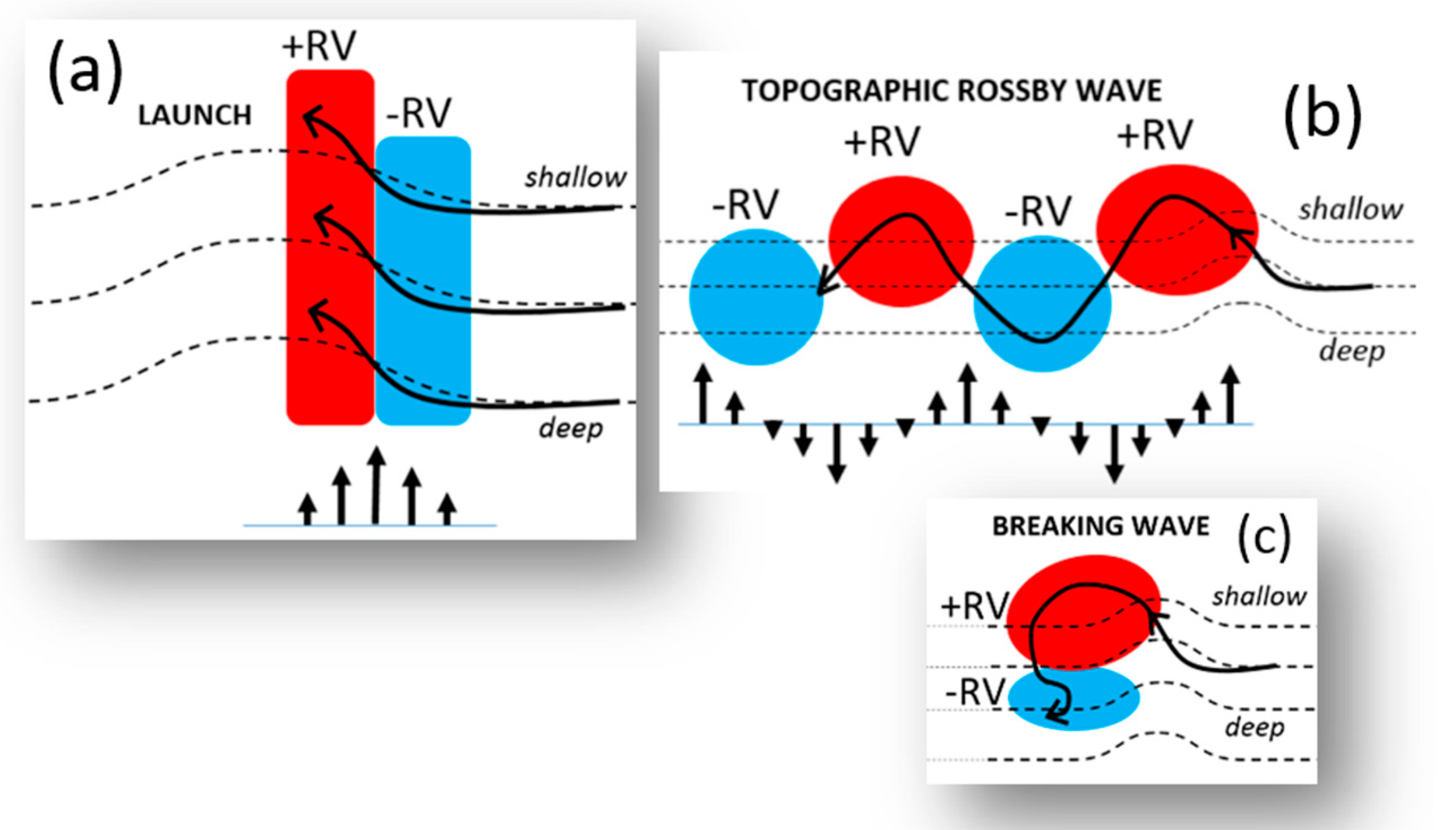
• Canyon upwelling is a signature of a stationary topographic Rossby wave forming downstream from the canyon. It exclusively develops for right-bounded (left-bounded) shelf-break flows in the southern (northern) hemisphere.
• The initial phase of canyon upwelling is a largely barotropic and friction-independent process and can be explained by the basic principle of conservation of potential vorticity.
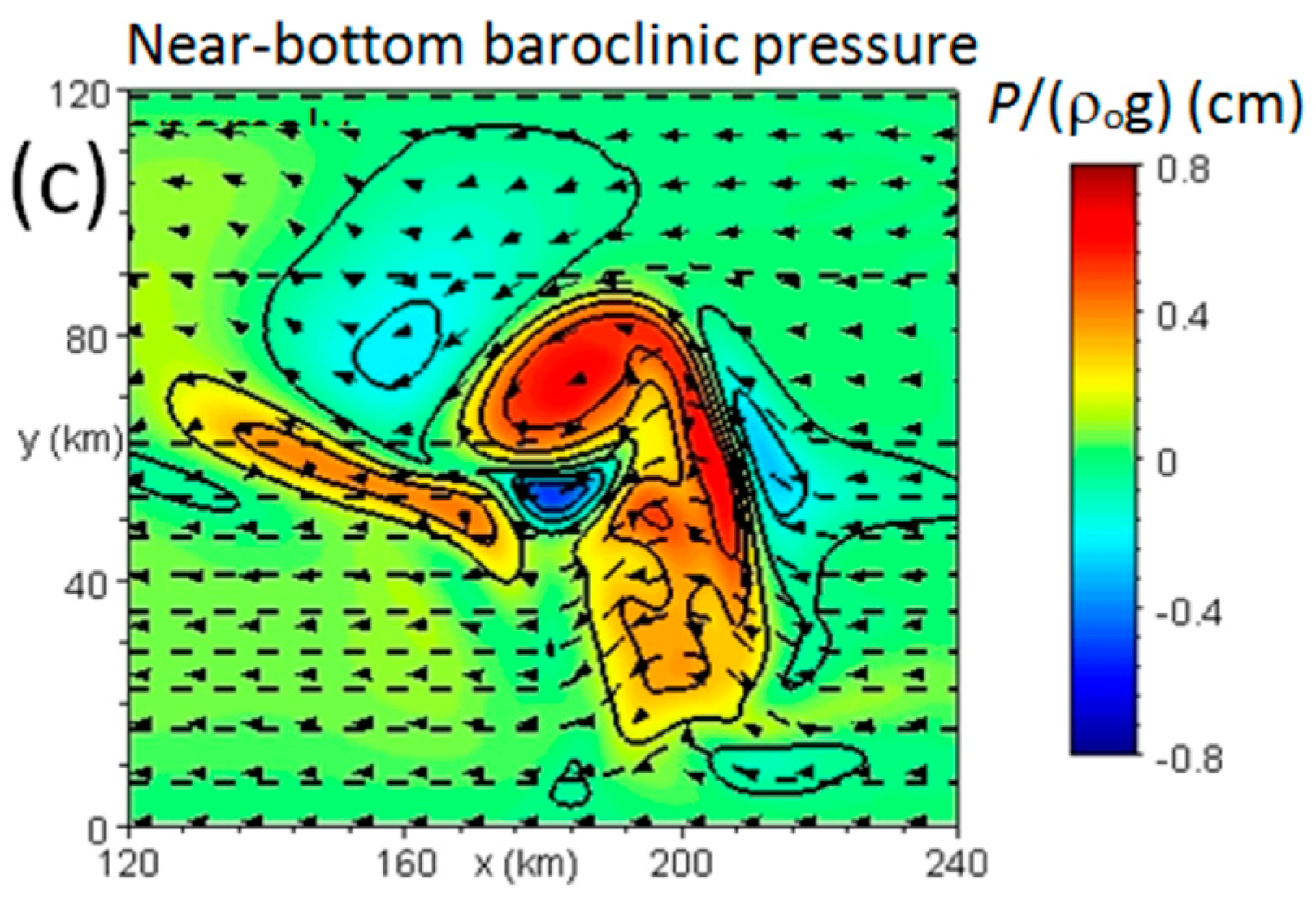
• Baroclinic geostrophic adjustment enhances canyon upwelling via the formation of narrow (~few km wide) frontal jets.

Indeed, barotropic topographic Rossby waves have been intensively studied for many decades. The pioneering work of Charney and Eliassen [16] demonstrated the orographic forcing of large-scale stationary Rossby-wave disturbances in the midlatitude westerlies. From the late 1960s onwards, oceanographers undertook similar studies on flow disturbances near seamounts (e.g., [17]) and submarine ridges (e.g., [18,19,20]). Dickinson [21] presented a comprehensive review of early research on Rossby waves in the oceans and the atmosphere. Previous research has shown that topographic obstacles such as islands [22] or headlands [23] can trigger stationary topographic Rossby waves on the continental shelf. Thus, it is not surprising to conclude (based on this work’s results) that such waves are also fundamental to the canyon–flow interaction process. It should be noted that a process-oriented modeling study [24] indicates that canyon-induced Rossby waves can trigger localized shelf-break upwelling at considerable distances (>100 km) from a canyon.

References

1. Baines, P.G.; Condie, S. Observations and modelling of Antarctic downslope flows: A review. In Ocean, Ice and Atmosphere: Interactions at the Continental Margin; Jakobs, S.S., Weiss, R., Eds.; Antarctic Research Series; AGU: Washington, DC, USA, 1998; Volume 15, pp. 29–49. [Google Scholar]
2. Kämpf, J.; Fohrmann, H. Sediment-driven downslope flow in submarine canyons and channels: Three-dimensional numerical experiments. J. Phys. Oceanogr. 2000, 30, 2302–2319. [Google Scholar] [CrossRef]
3. Hickey, B.M. The response of a steep-sided narrow canyon to strong wind forcing. J. Phys. Oceanogr. 1997, 27, 697–726. [Google Scholar] [CrossRef]
4. Allen, S.E.; Hickey, B.M. Dynamics of advection-driven upwelling over a submarine canyon. J. Geophys. Res. Oceans 2010, 115, C08018. [Google Scholar] [CrossRef]
5. Kämpf, J. On the preconditioning of coastal upwelling in the eastern Great Australian Bight. J. Geophys. Res. 2010, 115. [Google Scholar] [CrossRef]
6. Freeland, H.J.; Denman, K.L. A topographically controlled upwelling center off southern Vancouver Island. J. Mar. Res. 1982, 40, 1069–1093. [Google Scholar]
7. Kämpf, J. Transient wind-driven upwelling in a submarine canyon: A process-oriented modeling study. J. Geophys. Res. 2006, 111, 1–12. [Google Scholar] [CrossRef]
8. Kämpf, J. On the magnitude of upwelling fluxes in submarine canyons. Cont. Shelf Res. 2007, 27, 2211–2223. [Google Scholar] [CrossRef]
9. Sutherland, D.A.; Cenedese, C. Laboratory experiments on the interactions of a buoyant coastal current with a canyon: Application to the East Greenland Current. J. Phys. Oceanogr. 2009, 39, 1258–1271. [Google Scholar] [CrossRef]
10. Luyten, P.J.; Jones, J.E.; Proctor, R.; Tabor, A.; Tett, P.; Wild-Allen, K. COHERENS—A Coupled Hydrodynamical-Ecological Model for Regional and Shelf Seas: User Documentation; MUMM Report; Management Unit of the North Sea: Brussels, Belgium, 1999; 914p. [Google Scholar]
11. Kämpf, J. On the interaction of time-variable flows with a shelf-break canyon. J. Phys. Oceanogr. 2009, 39, 248–260. [Google Scholar] [CrossRef]
12. Pacanowsky, R.C.; Philander, S.G.H. Parameterization of vertical mixing in numerical models of tropical oceans. J. Phys. Oceanogr. 1981, 11, 1443–1451. [Google Scholar] [CrossRef]
13. Klinck, J. Circulation near submarine canyons: A modelling study. J. Geophys. Res. 1996, 101, 1211–1223. [Google Scholar] [CrossRef]
14. Cushman-Roisin, B. Introduction to Geophysical Fluid Dynamics; Prentice Hall: Upper Saddle River, NJ, USA, 1994; 320p. [Google Scholar]
15. Mirshak, R.; Allen, S.E. Spin-up and the effects of a submarine canyon: Application to upwelling in Astoria Canyon. J. Geophys. Res. 2005, 110, C02013. [Google Scholar] [CrossRef]
16. Charney, J.; Eliassen, A. A numerical model for predicting the perturbation of the middle latitude and westerlies. Tellus 1949, 1, 38–54. [Google Scholar] [CrossRef]
17. Huppert, H.E.; Bryan, K. Topographically generated eddies. Deep Sea Res. 1976, 23, 655–679. [Google Scholar] [CrossRef]
18. McIntyre, M.E. On stationary topography-induced rossby wave patterns in barotropic zonal current. Dtsch. Hydrogr. Z. 1968, 21, 203–214. [Google Scholar] [CrossRef]
19. Clark, R.A.; Fofonoff, N.P. Oceanic flow over varying bottom topography. J. Mar. Res. 1969, 27, 226–240. [Google Scholar]
20. Ikeda, M. Stationary rossby-waves in a two-layer model produced by a submarine ridge. J. Oceanogr. Soc. Jpn. 1979, 30, 100–109. [Google Scholar] [CrossRef]
21. Dickinson, R.E. Rossby waves—Long-period oscillations of oceans and atmospheres. Annu. Rev. Fluid Mech. 1978, 10, 159–195. [Google Scholar] [CrossRef]
22. Rhines, P.B. Jets and orography: Idealized experiments with tip-jets and lighthill blocking. J. Atmos. Sci. 2007, 64, 3627–3639. [Google Scholar] [CrossRef]
23. Freeland, H.J. The flow of a coastal current past a blunt headland. Atmos. Ocean 1990, 28, 288–302. [Google Scholar] [CrossRef] [Green Version]
24. Kämpf, J. Lee effects of localized upwelling in a shelf-break canyon. Cont. Shelf Res. 2012, 42, 78–88. [Google Scholar] [CrossRef]
Figure 1. Idealized bathymetry used in the control experiment of this study.
Jmse 06 00129 g001
Figure 2. Variations of ambient bathymetry (m) considered in sensitivity experiments.
Jmse 06 00129 g002
Figure 3. Variations of canyon shapes discussed in this paper. Shown are bathymetric transects along the shelf break at y = 60 km. The solid line represents the configuration of the control experiment. The dashed line denotes a box-type canyon considered in sensitivity studies.
Jmse 06 00129 g003
Figure 4. Control experiment: (a) offshore structure of ambient along-shore geostrophic flow; and (b) maximum possible water-column stretching Δh/hh, canyon depth; h, ambient total water depth). The star indicates the location of the shelf break.
Jmse 06 00129 g004
Figure 5. Topographic steering scenario. Trajectories of 3000 passive near-bottom drifters from day 5 to day 25 of the simulation. Black lines are isobaths. The arrow denotes the flow direction.
Jmse 06 00129 g005
Figure 6. Topographic steering scenario. Near-bottom anomalies of: (a) dynamic pressure converted to equivalent sea-surface elevation (cm); and (b) relative vorticity in units of |f|, both after 10 days of simulation. Ambient far-field distributions have been subtracted. Solid lines are isobaths. Arrows represent the near-bottom horizontal velocity field. Only every 8th vector is shown.
Jmse 06 00129 g006
Figure 7. Schematic of topographic steering for right-bounded flow in the northern hemisphere. Dashed lines are topographic contours. Circles are contours of dynamic pressure anomalies. Arrows are flow anomalies. The symbol “+” marks zones of positive relative vorticity. Zones of negative relative vorticity are marked by “−”. The thick line shows a selected flow trajectory. Numbers indicate different phases of the flow along this trajectory. During the canyon crossing (from Phase 1 to Phase 5), water-column squeezing creates a quasi-geostrophic flow that tends to align the flow trajectories with bathymetry contours. See text for more details.
Jmse 06 00129 g007
Figure 8. Canyon-upwelling scenario based on trajectories of 3000 passive near-bottom drifters from day 5 to day 25 of the simulation: (a) the result for the full model configuration; and (b) the result for a model run with uniform seawater density and zero friction. Black lines are isobaths. Arrows indicate the overall flow direction.
Jmse 06 00129 g008
Figure 9. Same as Figure 6a, but for the canyon-upwelling scenario after: (a) 5 days; and (b) 15 days.
Jmse 06 00129 g009
Figure 10. Same as Figure 6b, but for the canyon-upwelling scenario: (a) results for the full model configuration; and (b) results for the model run with uniform seawater density and zero friction. Note the variation of color ranges.
Jmse 06 00129 g010
Figure 11. Same as Figure 7, but for the canyon-upwelling scenario. The numbers denote different phases of the process. See text for more details.
Jmse 06 00129 g011
Figure 12. Schematics of different phases of the canyon-upwelling process: (a) the launch phase (Phases 1 → 2 in Figure 11); (b) the initiation of a topographic Rossby wave in the lee of the canyon; and (c) the possibility of breaking waves. Dashed lines are bathymetric contours. Long arrows indicate flow trajectories. Colored regions indicate zones of positive or negative relative vorticity (RV). Small arrows denote the structure of the cross-shelf flow. See text for further discussion.
Jmse 06 00129 g012
Figure 13. Canyon-upwelling scenario. Comparison between theoretical (L) and simulated wavelengths (L*) of pressure anomalies developing on the continental shelf in the lee of the shelf-break canyon.
Jmse 06 00129 g013
Figure 14. Canyon-upwelling scenario: (a) the surface pressure field in conjunction with surface currents; (b) the surface pressure anomalies (the upstream pressure field has been subtracted), again with surface currents; and (c) the baroclinic pressure component in conjunction with horizontal currents near the seafloor. Components of dynamic pressure (solid lines and color shading) and horizontal velocity fields (arrows) after 10 days of simulation. Every 8th vector is shown.
Jmse 06 00129 g014aJmse 06 00129 g014b
Figure 15. Canyon-upwelling scenario. The signature of shelf-break upwelling as seen in the near-bottom distribution of Eulerian tracer (color shading) after 20 days of simulation for: (a) the control experiment; and (b) a rectangular canyon (see Figure 4). Lines are bathymetric contours. Arrows represent the horizontal velocity field near the seafloor (only every 8th vector is shown).
Jmse 06 00129 g015