Spatio-Temporal Variations in Foredune Dynamics Determined with Mobile Laser Scanning


Abstract
1. Introduction
2. Materials and Methods
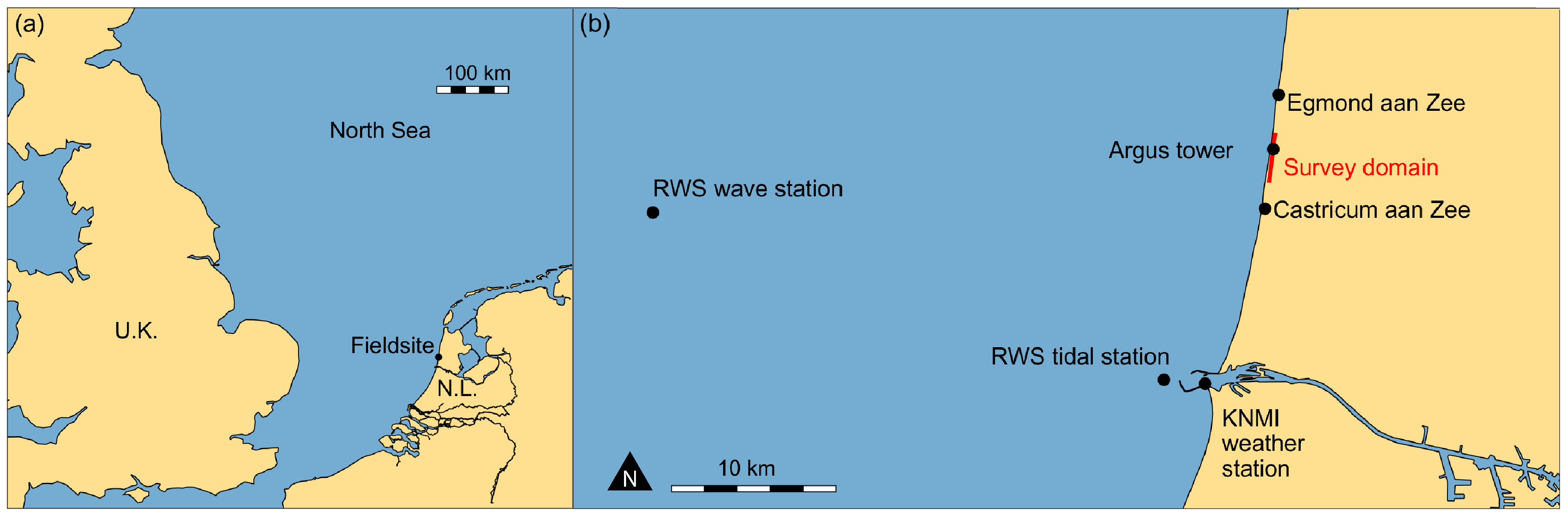
2.1. Field Location
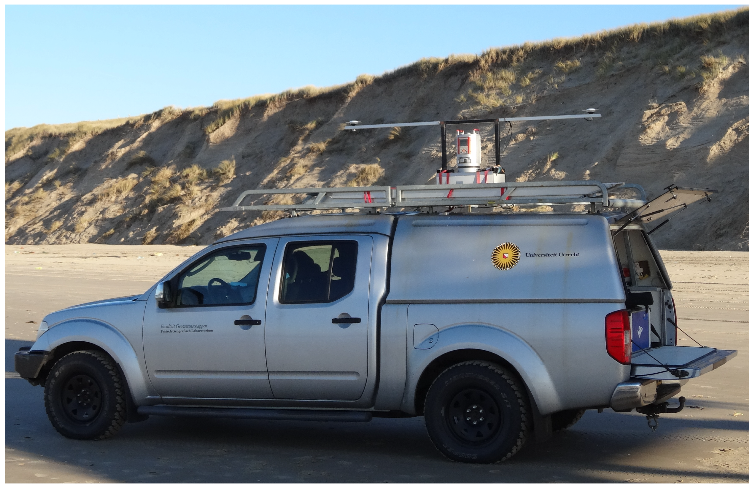
2.2. System and Data Collection
3. Error Analysis
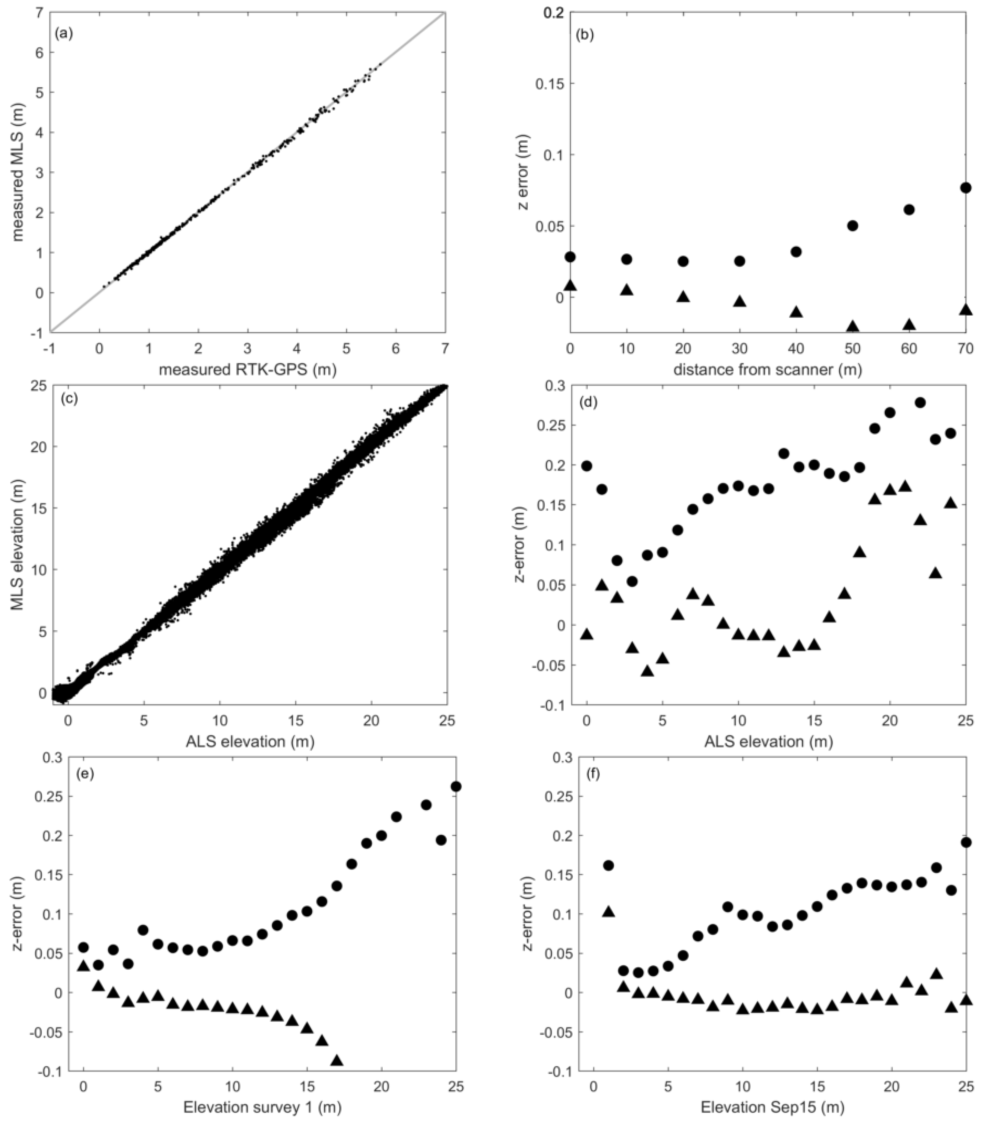
3.1. Validation
3.2. Robustness
4. Beach-Dune Dynamics
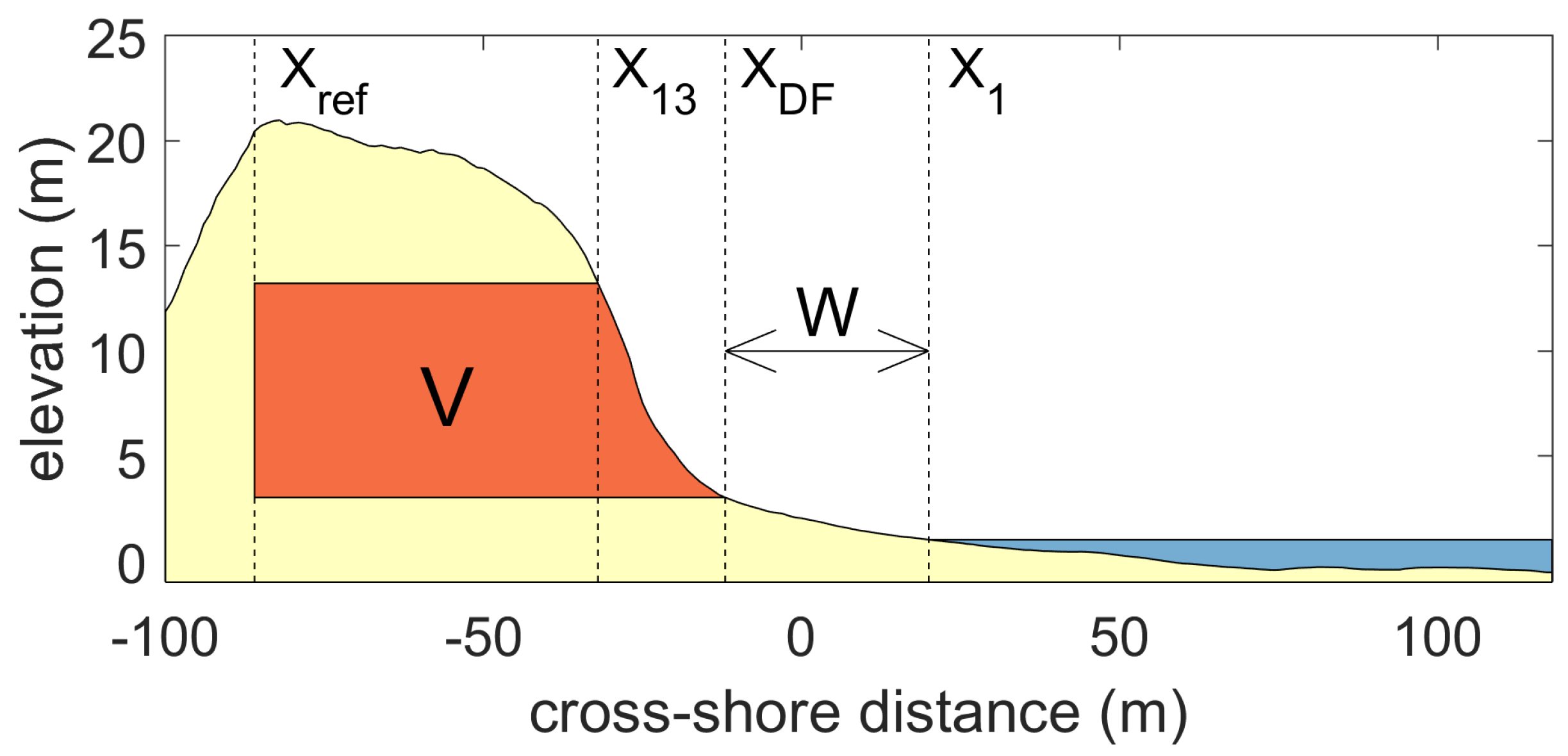
4.1. Methods
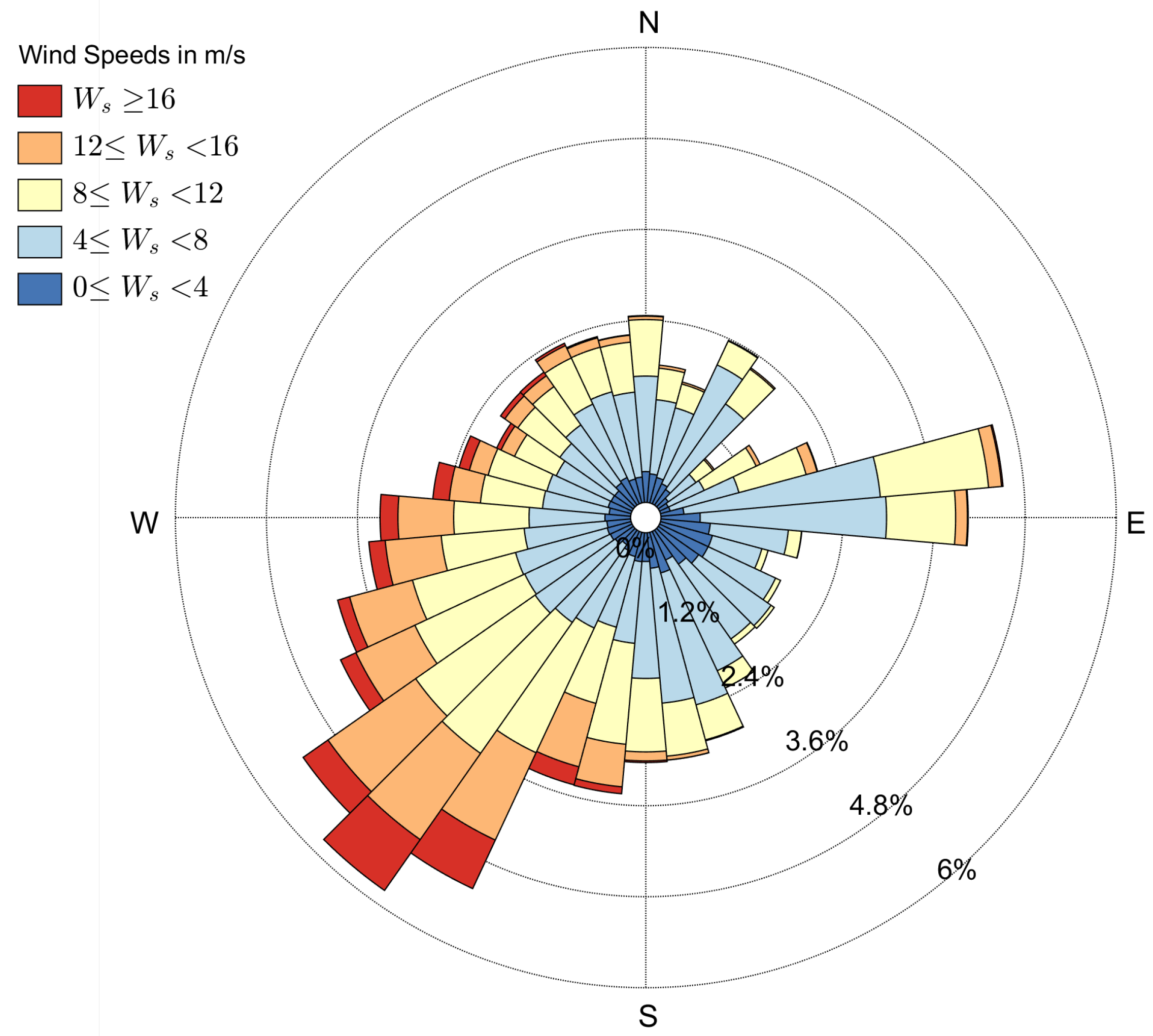
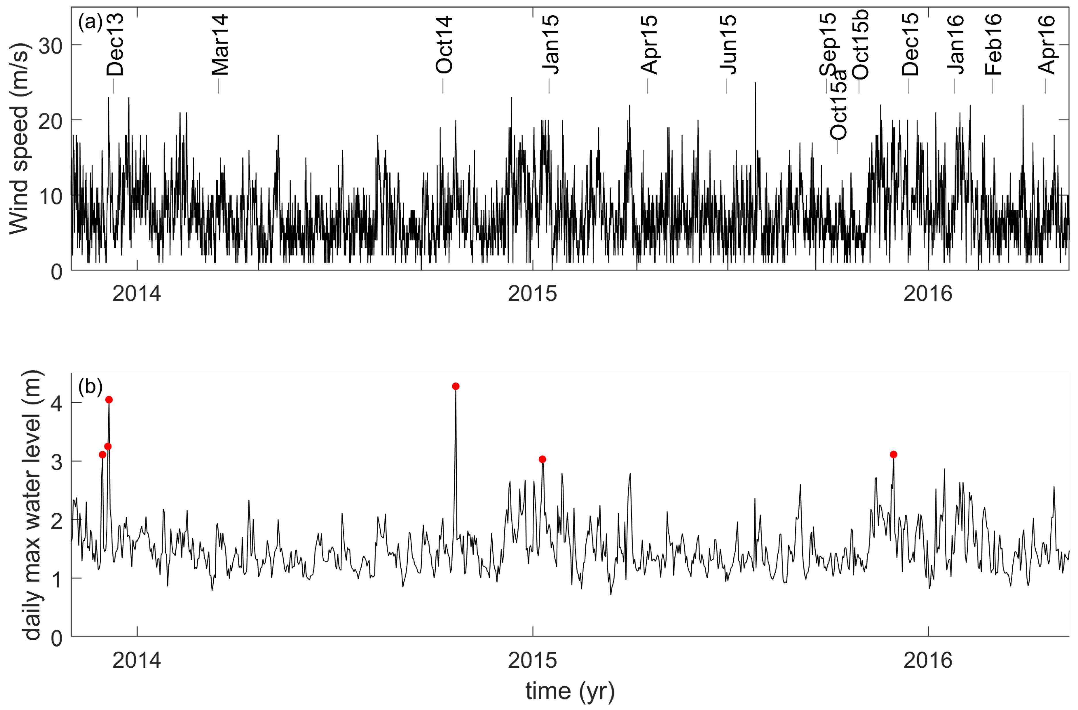
4.2. Conditions
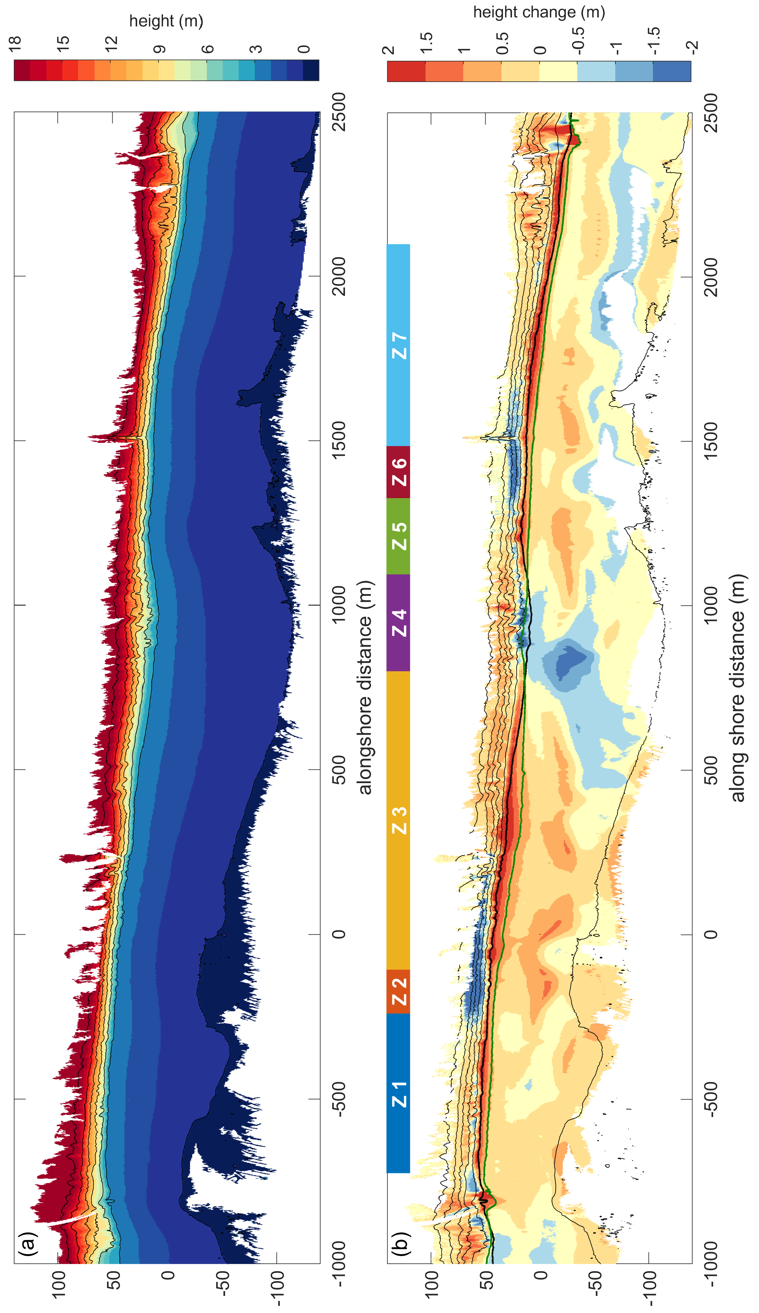
4.3. Topographic Changes
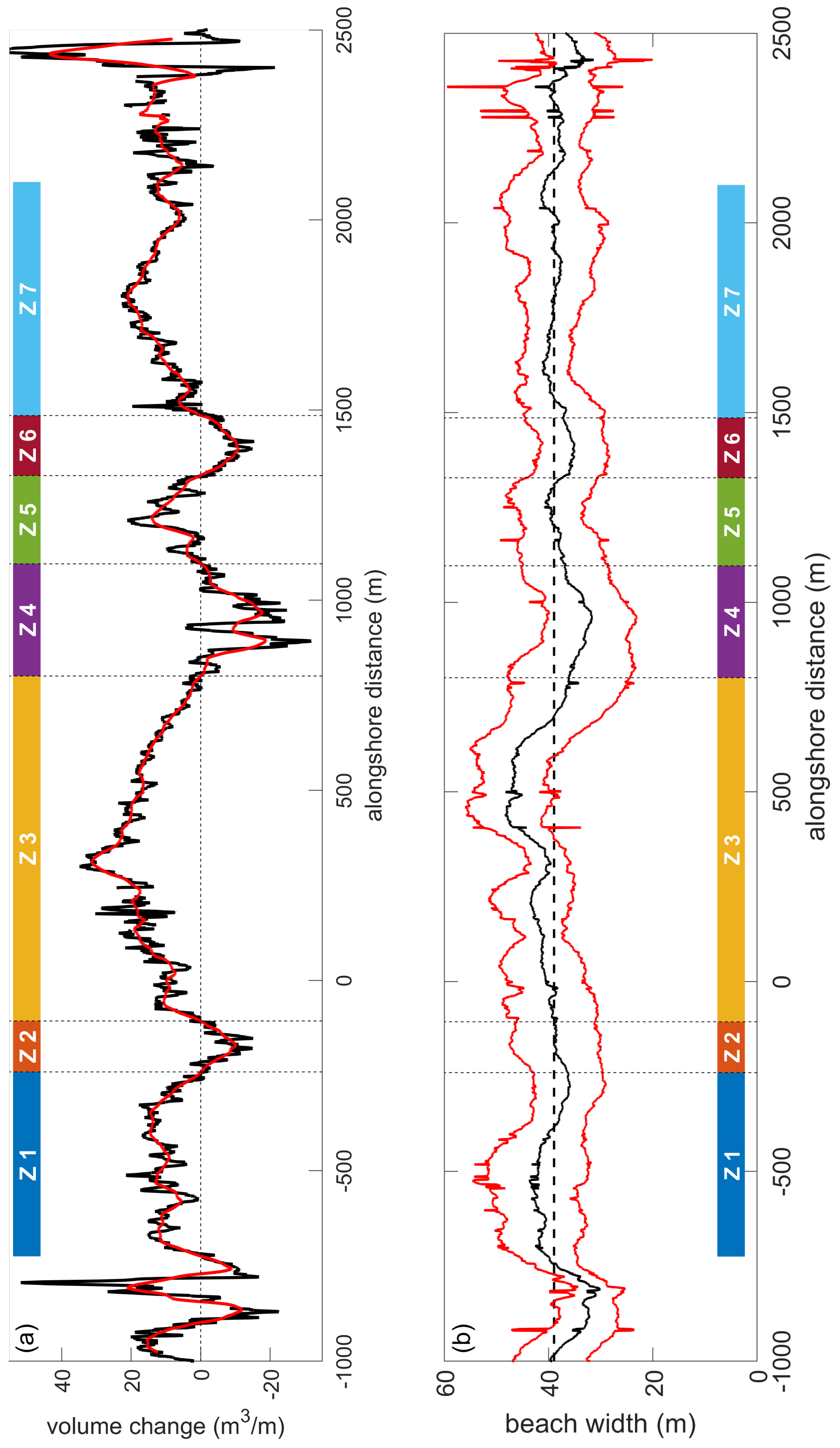
4.4. Spatio-Temporal Variation in Dune Volume Change
5. Discussion
5.1. Methodological Issues
5.2. Dune Dynamics
6. Conclusions
Author Contributions
Funding
Acknowledgments
Conflicts of Interest
Appendix A. Workflow
- The raw data gathered by the INS-GPS system and the external GPS correction data were post-processed in combined forward and backward mode using RT Post-Process software [48]. After data quality screening, a time-stamped position and orientation file was exported together with a second file containing time-stamped information on position and orientation accuracy. For the periods in which the data link with the RTK correction data service provider was lost, the post-processing procedure was slightly different. First, additional GNSS correction data was obtained in RINEX format. This correction data was also imported in the RT Post-Process software and used during the post-processing procedure.
- In the RiPROCESS software [49], the position and orientation file was imported into the project. The post-processed position and orientation file then overwrites the realtime position and orientation data linked to each point during the survey. Navigation data is linked to laser scan data using the recorded GPS time stamps.
- A transformation matrix containing the rotation and translation between the TLS and the INS-GPS measurement axes was applied to the position and orientation data to correct for the offset between both devices. A bore sighting procedure was performed to determine the pitch, roll and yaw offsets, needed to generate this transformation matrix, with high accuracy (details provided at the end of this Appendix).
- A georeferenced point cloud was generated from the survey data.
- The point cloud was filtered 4 times to classify points and to filter different types of noise. First, isolated points, defined as points with less than 5 neighboring points within a radius of 2 m, were detected. The next three filter steps were all performed using off-terrain filters, albeit used with different settings (see Table A1), for details on the working of each filter setting we refer to the help function of RiPROCESS sofware [49]. In short, the filter separates points from the underlying terrain by determining the distance of each point to an estimate of the ground surface. When the distance of a point to the estimated surface is larger than the given tolerance factor multiplied by the grid size, the point is filtered. The filter works in a hierarchic manner filtering the points at different spatial scales working from a coarse grid to the final base grid’s cell size. Grid sizes at each level can be calculated by multiplying the base grid size with 2, at each level the points falling outside the tolerance range are removed before continuing filtering at a lower level. At the second filter step the off-terrain filter was used with specific settings (vegetation) to delineate high vegetation and objects from terrain values. In the third step, the off-terrain point filter was applied to separate the terrain from the remaining low vegetation and other objects. In the final step, a fine filter was used to detect small-scale noise, for instance, caused by tire tracks. The filtered points were not removed but classified as isolated points [064], vegetation [003], non-terrain [001] and noise [037], respectively. The numbers indicate the classification codes. The Argus tower, and points reflected from the sea surface were classified manually as building [007] and water [009], respectively. The remaining non-classified points were classified as ground [002].
- The obtained point clouds were cut in tiles of 512 × 512 m and exported per survey record in a .las (1.4) format using the WGS84 datum. One tile may cover multiple passes. This results in separate files per pass.
- The tiled data was subsequently imported in Matlab® [50], and combined. Points classified as ground were extracted.
- A single return filter was applied on the extracted ground points to remove points from observations with multiple returns.
- The time stamp of each point was compared with the timeseries of position and orientation accuracy. Points were removed from the dataset for a 3D position error larger than 0.025 m, a heading error larger than 0.07 and a pitch/roll error larger than 0.03.
- The remaining points were transformed to the Dutch RD coordinate system, with the vertical reference point, called NAP (Amsterdam ordnance datum), having its zero level at Mean Sea Level. From the horizontal coordinates the location of the beach pole seaward of the Argus tower (102,572 m, 511,553 m) was subtracted, making the beach pole the local (0,0) coordinate. Subsequently, the grid was rotated by 172 degrees in clockwise direction, creating a cross—alongshore coordinate system in which the cross-shore-coordinate increases in the seaward direction and the alongshore-coordinate increases in the southward direction.
- The shifted and rotated points were then averaged on a 1 × 1 m grid by averaging all elevation z values (in NAP) of all points within a radius of 1 m from a grid point coordinate. Additionally, the number of data points and standard deviation of the point elevation was stored per grid cell.
- Small holes in the elevation model were replaced by means of smoothed interpolation using the values of neighbouring cells [51]. The final end products are digital models of elevation, point count and standard deviation in elevation.

| Vegetation | Terrain | Noise | |
|---|---|---|---|
| Base grid’s cell size | 0.25 m | 1 m | 0.25 m |
| Number of Levels | 8 | 4 | 4 |
| Tolerance factor | 0.7 | 1 | 0.7 |
| Percentile | 1% | 1% | 1% |
| Maximum slope angle | 60 | 90 | 90 |
| Fine filter tolerance filter | 0.1 m | 0.1 m | 0.05 m |
Bore Sighting Procedure
References
- Short, A.; Hesp, P. Wave, beach and dune interactions in southeastern Australia. Mar. Geol. 1982, 48, 259–284. [Google Scholar] [CrossRef]
- Durán, O.; Moore, L.J. Vegetation controls on the maximum size of coastal dunes. Proc. Natl. Acad. Sci. USA 2013, 110, 17217–17222. [Google Scholar] [CrossRef] [PubMed]
- Arens, S.M.; Wiersma, J. The Dutch foredunes: inventory and classification. J. Coast. Res. 1994, 10, 189–202. [Google Scholar]
- Everard, M.; Jones, L.; Watts, B. Have we neglected the societal importance of sand dunes? An ecosystem services perspective. Aquat. Conserv. Mar. Freshw. Ecosyst. 2010, 20, 476–487. [Google Scholar] [CrossRef]
- Carter, R.W.G.; Stone, G.W. Mechanisms associated with the erosion of sand dune cliffs, Magilligan, Northern Ireland. Earth Surf. Process. Landf. 1989, 14, 1–10. [Google Scholar] [CrossRef]
- De Winter, R.C.; Gongriep, F.; Ruessink, B.G. Observations and modeling of alongshore variability in dune erosion at Egmond aan Zee, The Netherlands. Coast. Eng. 2015, 99, 167–175. [Google Scholar] [CrossRef]
- Castelle, B.; Marieu, V.; Bujan, S.; Splinter, K.D.; Robinet, A.; Sénéchal, N.; Ferreira, S. Impact of the winter 2013–2014 series of severe Western Europe storms on a double-barred sandy coast: Beach and dune erosion and megacusp embayments. Geomorphology 2015, 238, 135–148. [Google Scholar] [CrossRef]
- Hesp, P. Foredunes and blowouts: Initiation, geomorphology and dynamics. Geomorphology 2002, 48, 245–268. [Google Scholar] [CrossRef]
- Roelvink, D.; Reniers, A.; van Dongeren, A.; van Thiel de Vries, J.; McCall, R.; Lescinski, J. Modelling storm impacts on beaches, dunes and barrier islands. Coast. Eng. 2009, 56, 1133–1152. [Google Scholar] [CrossRef]
- Thornton, E.B.; MacMahan, J.; Sallenger, A. Rip currents, mega-cusps, and eroding dunes. Mar. Geol. 2007, 240, 151–167. [Google Scholar] [CrossRef]
- Brodie, K.L.; Spore, N.J. Foredune classification and storm repsonse: Automated analysis of terrestrial LiDAR DEMS. In The Proceedings of the Coastal Sediments 2015; World Scientific: Singapore, 2015. [Google Scholar]
- Davidson-Arnott, R.G.D.; Law, M.N. Measurement and prediction of long-term sediment supply to coastal foredunes. J. Coast. Res. 1996, 12, 654–663. [Google Scholar]
- Delgado-Fernandez, I. A review of the application of the fetch effect to modelling sand supply to coastal foredunes. Aeolian Res. 2010, 2, 61–70. [Google Scholar] [CrossRef]
- Nordstrom, K.F.; Jackson, N.L. Effect of source width and tidal elevation changes on aeolian transport on an estuarine beach. Sedimentology 1992, 39, 769–778. [Google Scholar] [CrossRef]
- Bauer, B.O.; Davidson-Arnott, R.G. A general framework for modeling sediment supply to coastal dunes including wind angle, beach geometry, and fetch effects. Geomorphology 2003, 49, 89–108. [Google Scholar] [CrossRef]
- Walker, I.J.; Davidson-Arnott, R.G.; Bauer, B.O.; Hesp, P.A.; Delgado-Fernandez, I.; Ollerhead, J.; Smyth, T.A. Scale-dependent perspectives on the geomorphology and evolution of beach-dune systems. Earth-Sci. Rev. 2017, 171, 220–253. [Google Scholar] [CrossRef]
- Van der Wal, D. Effects of fetch and surface texture on aeolian sand transport on two nourished beaches. J. Arid Environ. 1998, 39, 533–547. [Google Scholar] [CrossRef]
- De Vries, S.; de Vries, J.V.T.; van Rijn, L.; Arens, S.; Ranasinghe, R. Aeolian sediment transport in supply limited situations. Aeolian Res. 2014, 12, 75–85. [Google Scholar] [CrossRef]
- Lynch, K.; Jackson, D.W.T.; Cooper, J.A.G. Aeolian fetch distance and secondary airflow effects: The influence of micro-scale variables on meso-scale foredune development. Earth Surf. Process. Landf. 2008, 33, 991–1005. [Google Scholar] [CrossRef]
- Guillén, J.; Stive, M.J.F.; Capobianco, M. Shoreline evolution of the Holland coast on a decadal scale. Earth Surf. Process. Landf. 1999, 24, 517–536. [Google Scholar] [CrossRef]
- Saye, S.; van der Wal, D.; Pye, K.; Blott, S. Beach–dune morphological relationships and erosion/accretion: An investigation at five sites in England and Wales using LIDAR data. Geomorphology 2005, 72, 128–155. [Google Scholar] [CrossRef]
- Claudino-Sales, V.; Wang, P.; Horwitz, M.H. Factors controlling the survival of coastal dunes during multiple hurricane impacts in 2004 and 2005: Santa Rosa barrier island, Florida. Geomorphology 2008, 95, 295–315. [Google Scholar] [CrossRef]
- Houser, C.; Hapke, C.; Hamilton, S. Controls on coastal dune morphology, shoreline erosion and barrier island response to extreme storms. Geomorphology 2008, 100, 223–240. [Google Scholar] [CrossRef]
- Mitasova, H.; Hardin, E.; Overton, M.F.; Kurum, M.O. Geospatial analysis of vulnerable beach-foredune systems from decadal time series of lidar data. J. Coast. Conserv. 2010, 14, 161–172. [Google Scholar] [CrossRef]
- Priestas, A.; Fagherazzi, S. Morphological barrier island changes and recovery of dunes after Hurricane Dennis, St. George Island, Florida. Geomorphology 2010, 114, 614–626. [Google Scholar] [CrossRef]
- Bochev-Van der Burgh, L.M.; Wijnberg, K.M.; Hulscher, S.J.M.H. Decadal-scale morphologic variability of managed coastal dunes. Coast. Eng. 2011, 58, 927–936. [Google Scholar] [CrossRef]
- Richter, A.; Faust, D.; Maas, H.G. Dune cliff erosion and beach width change at the northern and southern spits of Sylt detected with multi-temporal Lidar. Catena 2013, 103, 103–111. [Google Scholar] [CrossRef]
- Barber, D.M.; Mills, J.P. Vehicle based waveform laser scanning in a coastal environment. In Proceedings of the 5th International Symposium on Mobile Mapping Technology, Padua, Italy, 29–31 May 2007; Volume 36, p. C55. [Google Scholar]
- Bitenc, M.; Lindenbergh, R.; Khoshelham, K.; Van Waarden, A.P. Evaluation of a LIDAR Land-Based Mobile Mapping System for Monitoring Sandy Coasts. Remote Sens. 2011, 3, 1472–1491. [Google Scholar] [CrossRef]
- Aagaard, T.; Kroon, A.; Andersen, S.; Sørensen, R.M.; Quartel, S.; Vinther, N. Intertidal beach change during storm conditions; Egmond, The Netherlands. Mar. Geol. 2005, 218, 65–80. [Google Scholar] [CrossRef]
- Van Enckevort, I.M.J.; Ruessink, B.G. Effect of hydrodynamics and bathymetry on video estimates of nearshore sandbar position. J. Geophys. Res. Oceans 2001, 106, 16969–16979. [Google Scholar] [CrossRef]
- Glennie, C. Rigorous 3D error analysis of kinematic scanning LIDAR systems. J. Appl. Geod. 2007, 1, 147–157. [Google Scholar] [CrossRef]
- Ruessink, B.G.; Arens, S.M.; Kuipers, M.; Donker, J.J.A. Coastal dune dynamics in response to excavated foredune notches. Aeolian Res. 2018. [Google Scholar] [CrossRef]
- Stockdon, H.F.; Holman, R.A.; Howd, P.A.; Sallenger, A.H., Jr. Empirical parameterization of setup, swash, and runup. Coast. Eng. 2006, 53, 573–588. [Google Scholar] [CrossRef]
- Brakenhoff, L.B.; Smit, Y.; Donker, J.J.A.; Ruessink, B.G. Tide-induced variability in beach surface moisture: Observations and modelling. Earth Surf. Process. Landf. 2018. [Google Scholar] [CrossRef]
- Spencer, T.; Brooks, S.M.; Evans, B.R.; Tempest, J.A.; Möller, I. Southern North Sea storm surge event of 5 December 2013: Water levels, waves and coastal impacts. Earth-Sci. Rev. 2015, 146, 120–145. [Google Scholar] [CrossRef]
- Van de Graaff, J. Dune erosion during a storm surge. Coast. Eng. 1977, 1, 99–134. [Google Scholar] [CrossRef]
- Vellinga, P. Beach and dune erosion during storm surges. Coast. Eng. 1982, 6, 361–387. [Google Scholar] [CrossRef]
- Saarinen, N.; Vastaranta, M.; Vaaja, M.; Lotsari, E.; Jaakkola, A.; Kukko, A.; Kaartinen, H.; Holopainen, M.; Hyyppä, H.; Alho, P. Area-based approach for mapping and monitoring riverine vegetation using mobile laser scanning. Remote Sens. 2013, 5, 5285–5303. [Google Scholar] [CrossRef]
- Harding, D.J.; Lefsky, M.A.; Parker, G.G.; Blair, J.B. Laser altimeter canopy height profiles: Methods and validation for closed-canopy, broadleaf forests. Remote Sens. Environ. 2001, 76, 283–297. [Google Scholar] [CrossRef]
- De Vries, S.; Southgate, H.N.; Kanning, W.; Ranasinghe, R. Dune behavior and aeolian transport on decadal timescales. Coast. Eng. 2012, 67, 41–53. [Google Scholar] [CrossRef]
- Keijsers, J.G.S.; Poortinga, A.; Riksen, M.J.P.M.; Maroulis, J. Spatio-temporal variability in accretion and erosion of coastal foredunes in the netherlands: Regional climate and local topography. PLoS ONE 2014, 9, e91115. [Google Scholar] [CrossRef] [PubMed]
- Pye, K.; Blott, S.J. Assessment of beach and dune erosion and accretion using LiDAR: Impact of the stormy 2013–14 winter and longer term trends on the Sefton Coast, UK. Geomorphology 2016, 266, 146–167. [Google Scholar] [CrossRef]
- Psuty, N. The coastal foredune: A morphological basis for regional coastal dune development. In Coastal Dunes; Springer: Berlin/Heidelberg, Germany, 2008; pp. 11–27. [Google Scholar]
- Hoonhout, B.M.; Vries, S.D. A process-based model for aeolian sediment transport and spatiotemporal varying sediment availability. J. Geophys. Res. Earth Surf. 2016, 121, 1555–1575. [Google Scholar] [CrossRef]
- Davidson-Arnott, R.G.; Law, M.N. Seasonal patterns and controls on sediment supply to coastal foredunes, Long Point, Lake Erie. In Coastal Dunes: Form and Process; John Wiley & Sons: Hoboken, NJ, USA, 1990; pp. 177–200. [Google Scholar]
- Delgado-Fernandez, I. Meso-scale modelling of aeolian sediment input to coastal dunes. Geomorphology 2011, 130, 230–243. [Google Scholar] [CrossRef]
- OxTS. RT Post-Process Wizard; Oxford Technical Solutions Limited: Upper Heyford, UK, 2011. [Google Scholar]
- Riegl LMS GmbH. RiProcess Manual; Riegl LMS GmbH: Horn, Austria, 2014. [Google Scholar]
- MATLAB; Version 9.2.0 (R2017a); The MathWorks Inc.: Natick, MA, USA, 2017.
- D’rrico, J. Inpain Nans. Matlab Central File Exchange, Release: 2, 2004. Available online: https://nl.mathworks.com/matlabcentral/fileexchange/4551-inpaint_nans (accessed on 19 July 2008).
- Rieger, P.; Studnicka, N.; Pfennigbauer, M.; Zach, G. Boresight alignment method for mobile laser scanning systems. J. Appl. Geod. 2010, 4, 13–21. [Google Scholar] [CrossRef]


| Survey | Date | nr of Points | Points per m | Comments |
|---|---|---|---|---|
| Dec13 | 10-12-2013 | 636 × 10 | 964 | combines points from Dec13a and Dec13b |
| Dec13a | 10-12-2013 | 329 × 10 | 629 | |
| Dec13b | 10-12-2013 | 307 × 10 | 626 | driving path close to foredune |
| Mar14 | 17-03-2014 | 356 × 10 | 746 | Southern part is missing |
| Okt14 | 10-10-2014 | 355 × 10 | 1238 | |
| Jan15 | 16-01-2015 | 32 × 10 | 162 | Additional RTK-correction data obtained |
| Apr15 | 17-04-2015 | 210 × 10 | 402 | Additional RTK-correction data obtained |
| Jun15 | 29-06-2015 | 298 × 10 | 613 | |
| Sep15 | 29-09-2015 | 337 × 10 | 513 | Additional RTK-correction data obtained |
| Okt15a | 09-10-2015 | 248 × 10 | 524 | |
| Okt15b | 29-10-2015 | 361 × 10 | 795 | |
| Dec15 | 14-12-2015 | 384 × 10 | 431 | |
| Jan16 | 25-01-2016 | 359 × 10 | 391 | Additional RTK-correction data logged |
| Feb16 | 29-02-2016 | 372 × 10 | 421 | Additional RTK-correction data logged |
| Apr16 | 18-04-2016 | 289 × 10 | 336 | Additional RTK-correction data logged |
© 2018 by the authors. Licensee MDPI, Basel, Switzerland. This article is an open access article distributed under the terms and conditions of the Creative Commons Attribution (CC BY) license (http://creativecommons.org/licenses/by/4.0/).
Share and Cite
Donker, J.; Van Maarseveen, M.; Ruessink, G. Spatio-Temporal Variations in Foredune Dynamics Determined with Mobile Laser Scanning. J. Mar. Sci. Eng. 2018, 6, 126. https://doi.org/10.3390/jmse6040126
Donker J, Van Maarseveen M, Ruessink G. Spatio-Temporal Variations in Foredune Dynamics Determined with Mobile Laser Scanning. Journal of Marine Science and Engineering. 2018; 6(4):126. https://doi.org/10.3390/jmse6040126
Chicago/Turabian StyleDonker, Jasper, Marcel Van Maarseveen, and Gerben Ruessink. 2018. "Spatio-Temporal Variations in Foredune Dynamics Determined with Mobile Laser Scanning" Journal of Marine Science and Engineering 6, no. 4: 126. https://doi.org/10.3390/jmse6040126
APA StyleDonker, J., Van Maarseveen, M., & Ruessink, G. (2018). Spatio-Temporal Variations in Foredune Dynamics Determined with Mobile Laser Scanning. Journal of Marine Science and Engineering, 6(4), 126. https://doi.org/10.3390/jmse6040126