CMIP5-Derived Single-Forcing, Single-Model, and Single-Scenario Wind-Wave Climate Ensemble: Configuration and Performance Evaluation

Abstract

A Coupled Model Intercomparison Project Phase 5 (CMIP5)-derived single-forcing, single-model, and single-scenario dynamic wind-wave climate ensemble is presented, and its historic period (1979–2005) performance in representing the present wave climate is evaluated. A single global climate model (GCM)-forcing wave climate ensemble was produced with the goal of reducing the inter GCM variability inherent in using a multi-forcing approach for the same wave model. Seven CMIP5 EC-Earth ensemble runs were used to force seven WAM wave model realizations, while future wave climate simulations, not analyzed here, were produced using a high-emission representative concentration pathway 8.5 (RCP8.5) set-up. The wave climate ensemble’s historic period was extensively compared against a set of 72 in situ wave-height observations, as well as to ERA-Interim reanalysis and Climate Forecast System Reanalysis (CFSR) hindcast. The agreement between the wave climate ensemble and the in situ measurements and reanalysis of mean and extreme wave heights, mean wave periods, and mean wave directions was good, in line with previous studies or even better in some areas of the global ocean, namely in the extratropical latitudes. These results give a good degree of confidence in the ability of the ensemble to simulate a realistic climate change signal.

1. Introduction

Climate change extends beyond the scientific community, becoming a key topic in day-to-day public opinion. Matters like sea-level rise, ice-cap melting, extreme storms, droughts and floods, or coastal erosion, just to mention a few, are now common matters of discussion in the media or even in colloquial gatherings. Climate change adaptation and mitigation strategies also now raise increased societal interest. One of the key issues related to climate change, specifically ocean-related, is the potential increase of coastal hazards, like inundation or extreme coastal erosion, particularly when linked to sea-level rise, affecting coastal areas and low-land countries. Ocean surface gravity waves (or wind waves, as they are also called) can be classified as wind sea or swell, depending on their degree of coupling to the overlaying atmosphere [1]. Wind seas are young waves under the influence of the overlaying wind, directly receiving momentum from the atmosphere, to which they are strongly coupled [2,3]. Swell waves are mature waves that propagate away from their generation area by outrunning the overlaying wind speed. Swell waves can propagate thousands of kilometers, across entire ocean basins [4,5] with very little attenuation [4,6,7,8]. For this reason, the ocean surface wave field is the result of local and remotely generated waves, being strongly dominated by swell [3,9,10,11]. Therefore, wave climate variability in the open ocean, due to wave propagation characteristics, is often dominated by changes in swell waves carrying the effect of changes in surface winds into remote areas, contributing to changes in the wave climate elsewhere. For that matter, a direct link between the local wind speed and wave field’s long-term variabilities should be done with caution.

Wave climate is of fundamental importance to a variety of applications, like the design of offshore and coastal infrastructures, ship design standards, ship routing, and coastal management, among others. Wave climate is also a key factor in determining rates of coastal erosion and sediment budgets. The monitoring of present wave climate conditions is, therefore, a common practice, e.g. [3,7,12,13,14,15,16]. In face of a warming climate due to anthropogenic greenhouse gas emissions [17], a trend that will most probably continue until the end of the twenty-first century due to the inertia of the Earth’s climate and to additional greenhouse gas emissions [18], the study of the impact of climate change in future wave climate is of paramount importance. This study is also important from a scientific point of view, since waves play a key role in the climate system, modulating the exchanges of momentum, heat, and mass across the air–sea interface [14,19,20,21,22,23]. Waves also have an impact on the upper ocean layers and on trough wave-induced turbulence in the mixing layer; they are an important driver in defining the sea surface temperature, with direct impact on the lower atmosphere [24]. Changes in the future wave pattern can, therefore, play an important role in ocean surface heat fluxes.

Despite the role of waves in the climate system, up until today no fully coupled ocean-wave–atmosphere climate model exists, albeit some attempts, e.g. [23,25]. For that reason, global wave climate studies still rely on wind forcing (and sea ice coverage) from previous global climate model (GCM) simulations. The study of the impact of climate change on future wave conditions is done following one of two methods: dynamical, using physically based wave models, and statistical, using statistical models, both relying on a priori GCM simulations. Dynamical wave climate simulations use close-to-the-surface wind speeds (usually at 10-m height; $U_{10}$) and sea ice coverage (SIC) from GCMs to force a physical wave model. Statistical simulations, on the other hand, use mean sea level pressure (MSLP) or $U_{10}$ wind fields (and SIC) as input to statistical models. Each of the aforementioned methods has its advantages and limitations, with dynamical wave climate projections being computationally more expensive than statistical ones, although producing more accurate and physically sound results. The first dynamical global wave climate projections were done under the auspices of the Coordinated Ocean Wave Climate Project (COWCLIP), supported by the World Climate Research Program—Joint Technical Commission for Oceanography and Marine Meteorology (WCRP-JCOMM) [26,27]. Upon the work of [28], several other global future wave climate projections followed, e.g. [29,30,31,32,33,34], forced with Coupled Model Intercomparison Project Phases 3 and 5 (CMIP3 and CMIP5) GCM simulations. A concise review of the wave climate projections pursued in the recent past can be found in a review by [35].

Recent climate projections use ensembles instead of single GCM simulations. The use of ensembles has the goal of reducing uncertainties inherent to the simulations that arise from the GCM’s internal variability [36,37,38]. Uncertainties in climate modeling occur due to errors in the physical parameterizations of the models, to small-scale processes not fully understood, or to processes not resolved due to computational constraints [39]. These uncertainties are often a limiting factor in climate studies, particularly at regional scales [40,41,42]. By using the GCM ensemble approach, dedicated dynamic ensembles of wave climate simulations were also recently produced, e.g. [43,44,45]. These dedicated wave climate ensembles relied on multi-forcing suits, i.e., different GCMs were used in the same ensemble, providing forcing to a single wave model (dynamical simulations) or to a statistical model (statistical simulations).

In contrast to single wave climate runs and to multi-forcing (multi-GCM) dynamical or statistical ensemble studies of wave climate projections, a different approach was attempted in the present study, where a single-GCM-forced dynamic ensemble was used. An ensemble of seven independent CMIP5 climate simulations, produced with the same GCM (EC-Earth) [46] was used to force the third generation WAM wave model [47], with $U_{10}$ winds and SIC. The historic period of the seven wave climate simulations span from 1979 to 2005. The future wave climate simulations, not analyzed here, were produced using the EC-Earth representative concentration pathway (RCP8.5; [48]) set-up from 2006 to 2100. The ensemble described in this study is, therefore, a “single forcing-single (wave) model-single scenario” wave climate ensemble, produced with the goal of reducing the variability inherent in using a multi-forcing GCM approach for the same wave model, as in [43], for example.

The goal of this study was to present the single-forcing, single-model, and single-scenario wave climate ensemble design, and to assess its performance skills in reproducing the present time wave climate (as represented by the historic period). The ensemble historic period was extensively evaluated through comparison with a set of 72 in situ wave-height observations, with the European Centre for Medium-Range Weather Forecasts (ECMWF) ERA-Interim reanalysis [49], and the wave hindcast generated from the National Centre for Environmental Prediction (NCEP) Climate Forecast System Reanalysis (CFSR; [50]).

The remainder of the paper is structured as follows: in Section 2, the EC-Earth ensemble and the EC-Earth and WAM models, as well as the design of the dynamic wave climate ensemble, are described. The datasets used to evaluate the ensemble historic period (global wave reanalysis and hindcast, and in situ measurements) are also described in Section 2. The performance skills of the seven-member ensemble in representing present wind and wave climates are presented in Section 3. The summary and conclusions follow in Section 4.

2. Models, Data, and Methods

2.1. The EC-Earth GCM

The EC-Earth GCM, largely used in global and regional climate studies, e.g. [51], is a full physics seamless coupled atmosphere–ocean–sea ice–land earth system climate prediction model [46]. The EC-Earth was developed from the ECMWF operational seasonal forecast system 3 (ECMWF 2007), albeit with a different ocean model. The atmospheric model is the atmospheric component of the ECMWF Integrated Forecast System (IFS) cycle 31r1 (https://www.ecmwf.int/en/forecasts/documentation-and-support/changes-ecmwf-model/ifs-documentation, last accessed on June 2018). The ocean general circulation model in EC-Earth is the Nucleus for European Modeling of the Ocean (NEMO) version 2 (OPA9: Océan Parallélisé version 9), developed by the Institute Pierre Simon Laplace [52,53]. See [46] for further details on the EC-Earth performance skills, and [54] for further details on the NEMO ocean model in EC-Earth.

2.2. The WAM Wave Model

The WAM wave model version used here is cycle 4.5.3 (C4.5.3), an update of WAM cycle 4, described in [55,56]. WAM cycle 4.5.3 (C4.5.3) includes a source function integration scheme developed by [57], with a new semi-implicit approach developed at the ECMWF. The model updates described in the article by [58] are also included. Additionally, in WAM C4.5.3, the wind generation function and dissipation terms implement the [59,60,61] formulation, and the nonlinear interaction source functions are evaluated using the DIA (discrete interaction approximation) [62]. Additional details on WAM C4.5.3 can be seen in [63].

2.3. Experimental Set-Up

State-of-the-art comprehensive Earth system GCMs, such as the ones used in the CMIP5, rely on ensemble strategies for a more realistic approach to the variability, trends, and extremes of the past, present, and future of the Earth climate. The design of CMIP5 climate experiments [64] led to an extensive list of consistent and comparable GCM simulations of the Earth’s climate, under a number of present climate and future climate change scenarios as the RCPs [48]. Both multi-model ensemble and perturbed physics approaches were used in CMIP5 in order to study or potentially reduce uncertainties in the climate projections. In general, three sources of uncertainties can be distinguished: firstly, the internal model variability or the unforced climate variability; secondly, the uncertainties due to model architecture, parameterizations, and physics; and thirdly, the uncertainties in future emission scenarios [36]. The EC-Earth ensemble, used here to force the WAM wave model, followed a different approach, with the initialization date as the differentiating factor. The seven EC-Earth runs used to force the WAM wave model were taken from the larger EC-Earth ensemble prepared for CMIP5. Each EC-Earth ensemble member integration started in 1850, with the only difference being the initial conditions. The initial conditions are snapshots taken from the long pre-industrial control simulation for CMIP5, each separated by 25 years.

The standard set-up of the atmospheric model in the EC-Earth version 2.2 corresponds to a triangular truncation at wavenumber 159 (T159) horizontal spectral resolution (about 125 km at the equator) and a vertical grid spacing with 62 vertical levels of terrain-following mixed sigma-pressure hybrid coordinates, of which about 15 are within the planetary boundary layer. Six of the seven EC-Earth runs used the standard vertical level set-up, while a seventh run, produced at the Danish Meteorological Institute (DMI) was set with an increased number of vertical levels as a differentiating factor. These levels were added in the stratosphere, and the top level of the EC-Earth was raised from 5 hPa to 0.1 hPa.

NEMO, the ocean component of EC-Earth, uses a horizontal resolution of roughly $1°\times 1°$ and 42 vertical layers. The past and present climate EC-Earth ensemble simulations cover the period between 1850 and 1855 to 2005. The future climate runs span from 2006 to 2100, following the RCP8.5 high-emission scenario [65].

Six-hourly 10-m wind speeds ($U_{10}$ ) and daily SIC (grid cells with ice coverage less than 0.5 were taken as no ice) with a horizontal resolution of about $1°\times 1°$, from the seven EC-Earth runs, were used to force seven realizations of the WAM wave model. The WAM runs were performed on a regular global latitude–longitude grid, covering a latitude range of 78° N to 78° S, with a fixed spatial grid size of $1°\times 1°$. The spectral domain was discretized into 25 logarithmically spaced frequency bins, from 0.041 Hz to 0.411 Hz, equivalent to wavelengths from about 10 to 950 m. Wave propagating directions were set with a resolution of 15°. The WAM model was run in shallow-water mode. The 1-min (~0.0168°) world-gridded elevations/bathymetry ETOPO1 data [66,67] were used to define the depths. The wave model runs were performed using integration time steps of 5 and 10 min for the advection and the source functions, respectively. A suit of 30 wave parameters, in addition to the neutral 10-m wind speed derived from different forms of integrating the outputted wave spectra, were stored every 6 h (see

Table A1. Integrated output parameters.

Parameter Number	Parameter	Dimensions
1	Wind speed $U_{10}$	ms−1
2	Wind direction $\phi$	degrees from north (toward)
3	Friction velocity	ms−1
4	Drag coefficient	m
5	Significant wave height	m
6	Total peak period	s
7	Total mean period	s
8	Total Tm1 period	s
9	Total Tm2 period	s
10	Total mean wave direction	degrees from north (toward)
11	Total directional spread	degrees
12	Normalized wave stress	%
13	Sea significant wave height	m
14	Sea peak period	s
15	Sea mean period	s
16	Sea Tm1 period	s
17	Sea Tm2 period	s
18	Sea mean wave direction	degrees from north (toward)
19	Swell significant wave height	m
20	Swell peak period	s
21	Swell mean period	s
22	Swell Tm1 period	s
23	Swell Tm2 period	s
24	Swell mean wave direction	degrees from north (toward)
25	Goda peakness parameter	-
26	Kurtosis	-
27	Benjamin Feir index	-
28	Normalized maximum wave height	m
29	Maximum wave period	s
30	Interpolated peak frequency	Hz
31	Peak direction	degrees from north (toward)
32	Mean square slope	-

in the Appendix). Having used the same GCM with the same RCP scenario to force a sole wave model, the ensemble described here qualifies as a “single-forcing, single-model, single-scenario” dynamic wave climate ensemble.

The WAM realizations were run for the present climate 20th century 1979–2005 period (the historic period). The WAM future climate 21st simulations were run for the 21th century 2006–2100 period. For convenience, the present climate simulations are named in general as PC20, the present climate historic ensemble is named PC20-E, and the individual ensemble members are named PC20-i (where i = 1 to 7). The future climate simulations (not analyzed here) are, on the other hand, named FC21, FC21-E, and FC21-i. Also for convenience, the EC-Earth $U_{10}$ wind-speed fields were included in PC20.

Table 1. Ensemble details: UL (University of Lisbon), UH (University of Hamburg), SMHI (Swedish Meteorological and Hydrological Institute), DMI (Danish Meteorological Institute), HZG (Helmholtz-Zentrum Geesthacht). PC20—present climate 20th century; FC21—future climate 21st century.

Ensemble Member	EC-Earth Run	WAM Run	PC20	FC21
1	UL	UL-HZG	1979–2005	2006–2100
2	DMI	UH	1979–2005	2070–2100
3	DMI	UH	1979–2005	2070–2100
4	SMHI	UH	1979–2005	2006–2100
5	SMHI	UH	1979–2005	2006–2100
6	DMI	UH	1979–2005	2070–2100
7	SMHI	UH	1979–2005	2006–2100

presents additional details on the EC-Earth and WAM runs, including the climate centers or research groups responsible for each of the EC-Earth ensemble members.

2.4. Global Evaluation Data: ERA-Interim Reanalysis and CFSR Hindcast

The performance skills of PC20-E were evaluated through comparison with the ECMWF ERA-Interim reanalysis (Dee et al., 2011) and with the National Oceanic and Atmospheric Administration (NOAA) CFSR wave hindcast [68]. The ensemble significant wave heights ($H_s$) were compared to ERA-Interim and CFSR. The mean wave periods ($T_m)$, mean wave directions (${\theta }_m$), and $U_{10}$ were compared only to ERA-Interim.

The ERA-Interim is a global third-generation reanalysis, produced at the ECMWF using the IFS release cycle Cy31r2 (https://www.ecmwf.int/en/forecasts/documentation-and-support/changes-ecmwf-model/ifs-documentation, last accessed on June 2018), used operationally at ECMWF during the period from December 2006 to June 2007. Here, we used the ERA-Interim period from 1979 to 2005. In addition to atmospheric variables, the ERA-Interim also includes reanalyzed wave parameters, since it was produced using the IFS, a two-way coupled atmosphere–wave model system [69]. The wave model used in this coupled model system is also a modified version of the WAM model (the so called EC-WAM), albeit different from WAM cycle 4.5.3. ERA-Interim uses an improved data assimilation technique in four dimensions (4D-Var scheme), which outperforms the previous three-dimensional (3D)-Var assimilation technique [70]. ERA-Interim assimilates surface wind speed observations from voluntary observing ships (VOS), buoys, and satellite scatterometery. Satellite altimetry wave heights were also assimilated since 1991. In situ $H_s$ measurements and altimeter winds at 10-m height are not used in the ERA-Interim; thus, they can be used to independently evaluate the merits of the reanalysis. The resolution of the atmospheric model component in ERA-Interim is about 79 km (T255 spectral truncation; ~0.7° × 0.7°), with 60 vertical levels from the surface up to 0.1 hPa. The wave model is set for a resolution of 110 km (~1° × 1°). The temporal resolution of ERA-Interim is 6 h. Additional details about the ERA-Interim reanalysis and its comparison with other global wave hindcasts can be found in articles by [16,49,71,72].The CFSR is the global NCEP third-generation reanalysis [68], produced with a coupled atmosphere–ocean–land surface–sea ice model system. The atmospheric component is the NOAA operational Global Forecast System (GFS). The ocean model coupled to the GFS in the coupled model system is the Geophysical Fluid Dynamics Laboratory (GFDL) Modular Ocean Model (MOM) version 4p0d [73]. The operational Global Data Assimilation System (GDAS) is used in the assimilation process. The CFSR global atmosphere resolution is ~38 km (T382), with 64 vertical levels up to 0.1 hPa. The global ocean is 0.25° at the equator, extending to a global 0.5° beyond the tropics with 40 levels. The CFSR reanalysis output is at a T382L64 resolution (~0.5° × 0.5° horizontal, ~0.266 hPa vertical), running originally from 1979 to 2009. From the CFSR atmospheric reanalysis dataset, a wave hindcast was produced [74] using the WAVEWATCH III wave model (WW3; [75]), the so-called CFSR wave hindcast. Here, we used the three-hourly CFSR hindcast (henceforth just called CFSR, or CFSR hindcast) global domain at a 0.5° × 0.5° horizontal resolution from 1979 to 2005. Additional details on the CFSR hindcast and its comparison with other global wave data sets can be found in the article by [72].

From here onward, the ERA-Interim reanalysis and the CFSR hindcast are interchangeably referred to as simply “reanalysis”, unless they need to be distinguished.

2.5. In Situ Evaluation Data: Wave Observations

The PC20-E significant wave heights ($H_s$) were also evaluated through comparison with 72 in situ observations, quality-controlled at the ECMWF, and regularly used to evaluate the wave forecasting scores of the operational IFS [76]. From all the in situ measurements available globally since 1979, 72 locations, with a long enough spanning time-series (at least 10 years) and positioned in relatively deep waters, were selected. Figure 1 shows these locations (see also

Table A2. In situ and buoy wave measurements details. Position refers to the mean position of the buoy during its time series. WMO—World Meteorological Organization.

WMO ID	Position	Time Series (Years)	WMO ID	Position	Time Series (Years)
41004	32.47° N, 78.90° W	37	46035	57.01° N, 177.70° W	30
41006	29.32° N, 77.35° W	14	46036	48.35° N, 133.92° W	29
41009	28.51° N, 80.19° W	27	46041	47.36° N, 124.63° W	28
41013	33.44° N, 77.66° W	12	46042	36.78° N, 122.35° W	28
41025	35.08° N, 75.35° W	12	46047	32.55° N, 119.55° W	24
41041	14.35° N, 46.05° W	10	46054	34.25° N, 120.45° W	22
42001	25.92° N, 89.93° W	36	46059	38.04° N, 129.95° W	21
42002	25.64° N, 93.96° W	36	46063	34.27° N, 120.68° W	10
42003	25.91° N, 85.50° W	37	46066	52.70° N, 154.98° W	15
42019	27.91° N, 95.20° W	26	46069	33.68° N, 120.20° W	12
42020	26.97° N, 96.60° W	26	46075	53.92° N, 160.81° W	11
42035	29.13° N, 94.60° W	22	46082	59.66° N, 143.54° W	13
42036	28.51° N, 84.51° W	22	46083	58.25° N, 138.00° W	14
42040	29.01° N, 88.15° W	20	46086	32.50° N, 118.02° W	12
42056	19.85° N, 85.00° W	10	46132	49.73° N, 127.93° W	22
44004	38.69° N, 70.36° W	29	46147	51.82° N, 131.22° W	22
44009	38.48° N, 74.65° W	19	46184	53.93° N, 138.84° W	28
44011	41.09° N, 66.59° W	21	46205	54.22° N, 133.86° W	27
44014	36.60° N, 74.82° W	25	46206	48.87° N, 126.00° W	27
44017	40.70° N, 72.03° W	13	46207	50.88° N, 129.91° W	26
44024	42.30° N, 65.90° W	11	46208	52.51° N, 132.69° W	25
44025	40.25° N, 73.19° W	24	46213	40.30° N, 124.72° W	16
44027	44.29° N, 67.31° W	12	46214	37.93° N, 123.49° W	19
44138	44.25° N, 53.62° W	22	46218	34.48° N, 120.75° W	20
44139	44.21° N, 57.36° W	25	51202	21.41° N, 157.69° W	15
44251	46.45° N, 53.39° W	18	62023	51.40° N, 7.90° W	15
46001	56.15° N, 148.10° W	36	62107	50.10° N, 6.10° W	21
46003	51.92° N, 155.85° W	19	62116	57.90° N, 1.45° E	11
46004	50.95° N, 135.96° W	37	62133	57.15° N, 0.95° E	17
46005	46.05° N, 131.00° W	35	62144	53.89° N, 1.54° E	17
46006	40.85° N, 137.70° W	37	62145	53.21° N, 2.59° E	17
46012	37.41° N, 122.78° W	35	LF4B	60.60° N, 3.70° E	17
46013	38.22° N, 123.32° W	34	TFBLK	65.70° N, 24.80° W	13
46015	42.75° N, 124.83° W	13	TFGSK	64.10° N, 22.90° W	13
46026	37.75° N, 122.76° W	33	TFKGR	65.65° N, 13.60° W	13
46028	35.75° N, 121.80° W	32	TFSRT	63.30° N, 20.30° W	13

for additional details).

2.6. Methodology

The PC20-E was built using a “democratic approach”, with an unweighted mean of the seven ensemble members (PC20-1 to 7) for the period from 1979 to 2005. The six-hourly wind and wave parameters are processed for annual and seasonal means: December to February (DJF), March to May (MAM), June to August (JJA), and September to November (SON). Here, only the extreme seasons DJF and JJA were analyzed.

In the high latitudes, natural variations in SIC extent can seriously affect the quality of mean wave fields, due to a considerable reduction of data points available, since the grid cells are taken as land by the wave model when covered with ice for an area higher than 50%. This situation was dealt with using one of the procedures proposed by [77] to treat wave statistics for climate purposes. Grid cells with full ice concentration for 30% of the time or more in the scrutinized periods were taken as land, and were ruled out of the statistics. For that matter, only cells with full ice concentration for 70% or more of the total time series were treated as open water.

For the comparison of PC20-E (and reanalysis) with the in situ observations, the observational and the modeled data were averaged on a daily basis. The ensemble and the reanalysis data were collocated with the wave observations through interpolation of the nearest grid points (bilinear interpolation) into the in situ observational positions.

The PC20-E performance skills were evaluated using the following standard statistics: bias—Equation (1), root-mean-square error (RMSE)—Equation (2), mean annual variability (MAV)—Equation (3), and the Arcsin–Mielke score (M-Score)—Equation (4), all of which are defined below.

$$Bias=\frac{1}{N}{{\displaystyle \sum }}_{i=1}^N\left(PC{20}_i-R_i\right),$$

(1)

$$RMSE=\sqrt{\frac{{{\displaystyle \sum }}_{i=1}^N{\left(PC{20}_i-R_i\right)}^2}{N}},$$

(2)

where $N$ is the number of realizations and $R$ is the reference data (in this case from observations or reanalysis). The MAV [18,72], which is an average of the annual standard deviation normalized by the annual mean, provides an indication of the spread of a climate simulation along the year and also its ability to simulate the seasonal extremes, and it is defined as

$$MAV=\frac{1}{M}\frac{{{\displaystyle \sum }}_{j=1}^M\sqrt{\frac{1}{N}{{\displaystyle \sum }}_{i=1}^N{\left(PC{20}_{ji}-\left(\frac{1}{N}{{\displaystyle \sum }}_{i=1}^{N}PC{20}_{ji}\right)\right)}^2}}{\frac{1}{N}{{\displaystyle \sum }}_{i=1}^{N}PC{20}_{ji}}=\overline{\left(\frac{{\sigma }_j}{\overline{PC{20}_j}}\right)},$$

(3)

where $M$ is the number of years in the record and $j$ is the position inside each year.

The non-dimensional Arcsin–Mielke score, or M-Score [78,79], used previously for wave climate parameters by [43], is defined as

$$M=\frac{2}{\pi }arcsin\left(1-\frac{MSE}{V_{pc20}+V_R+{\left(G_{PC20}+G_R\right)}^2}\right)\times 1000$$

(4)

where $MSE$ is the mean-square error, $V$ is the spatial variance, and $G$ is the spatial mean, either of PC20-E or the reanalysis. The M-Score varies from zero (no skill) to a maximum score of 1000 (for virtually no error, i.e., $MSE=0$). With the $\mathrm{arcsine}$ transformation of the Mielke skill score, introduced by [80], the deviation from unity asymptotes to the $RMSE$. The statistics were computed for the global ocean, and separately for 13 regional sub-areas, allowing the assessment of the ensemble’s regional performance. Each of these regions, chosen in accordance with [4], can be seen in Figure 1, with further details in

Table A3. Regional area limits from Figure 1, as in Alves et al. 2006. LAT—latitude; LON—longitude.

AREA	LAT (°)	LON (°)
ETSI	78° S–25° S	21° E–145° E
ETSP	78° S–25° S	145° E–70° W
ETSA	78° S–25° S	69° W–20° E
TSIO	24° S–0°	21° E–(100° E (N); 135° E (S))
TWSP	24° S–0°	(101° E (N); 136° E (S))–130° W
TESP	24° S–0°	129° W–65° W
TSAO	24° S–0°	64° W–20° E
TNIO	1° N–30° N	41° E–100° E
TWNP	1° N–30° N	101° E–180° E
TENP	1° N–30° N	Land
TNAO	1° N–38° N	(101° W (N); 69° W (S))–40° E
ETNP	31° N–78° N	101° E–102° W
ETNA	39° N–78° N	101° W–100° E

.

Numerical weather prediction (NWP) strategy has data assimilation as a key element. In climate studies, data assimilation is not present, and climate simulations do not capture the exact time history of the simulated parameters, making the comparison with observations or reanalysis a challenging task. Previous studies used the same overlapping period when comparing present climate wave simulations with reanalysis, e.g., [43], when that was possible. Other studies assumed that wave climate historic simulations, because they are not time-constrained, do not necessarily reproduce the exact same period as the referenced reanalysis; as such, they did not make these periods coincident, e.g., [33]). The problem is enhanced when the comparison is done with observations, e.g., in situ measurements or remote sensing. Most of the time, the periods and the lengths of the climate simulations do not coincide with the observational ones, which can pose additional challenges. That is the case, for example, with in situ observations that are either shorter in time length or have gaps in the data. Differences can also occur in comparisons with remote-sensing observations, which can also have different time lengths compared to climate simulations, or different time resolutions, typically lower than the climate simulations. For that reason, the simple comparison between observations and climate simulations is unfair (to the observations), since, even for overlapping time-slices, the density of the observations is typically lower. A technique where this “unfairness” is corrected, and the historic climate simulation output numbers (densities) and lengths (time-slices) are matched with the observational ones by randomly sampling the climate simulation data, was developed by [80]. Here, we used a similar approach to the comparison between PC20-E and in situ observations (intra-annual variability). To coincide the amount (number of observations and model outputs) and length of the in situ observations with the PC20, ten random Monte Carlo samples were taken of the climate data, and then averaged. This was done for each set of the 72 in situ observations.

3. Evaluation of the Wave Climate Simulation in the Historic Period

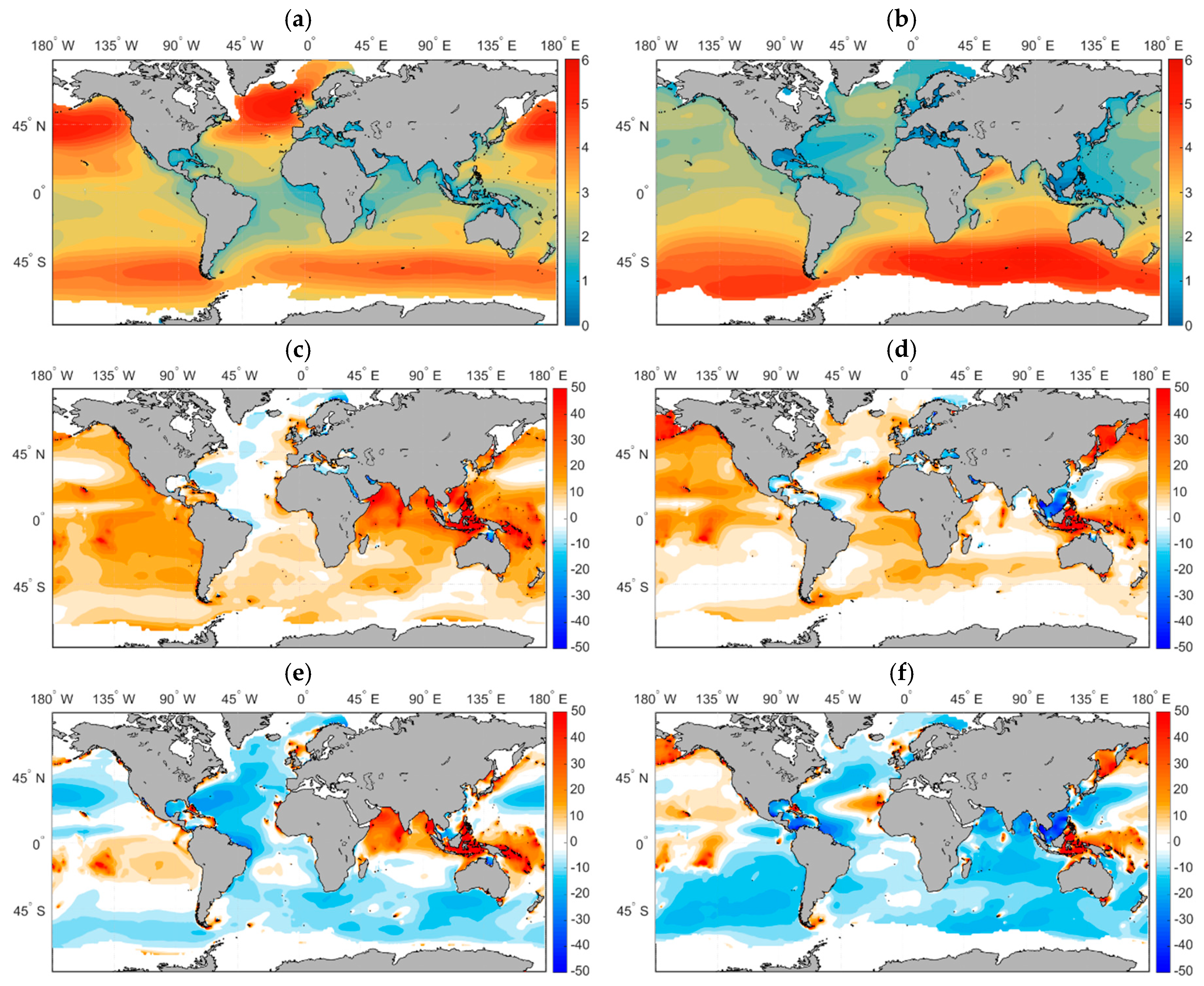
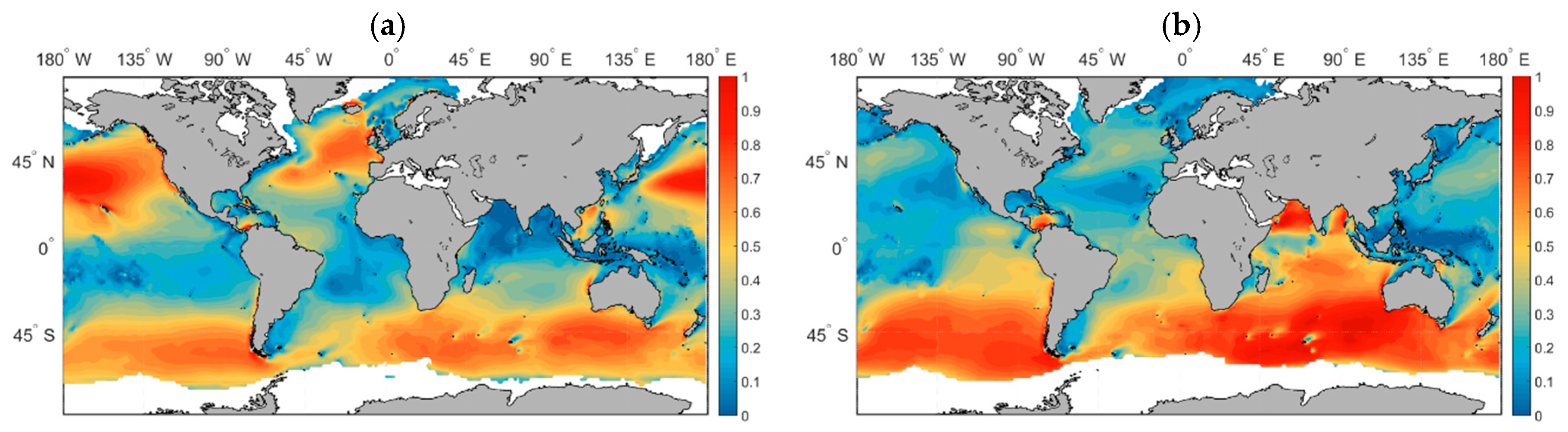
Firstly, the PC20-E was evaluated through comparison with the $H_s$ ERA-Interim and CFSR DJF and JJA global climatological means, as seen in the normalized differences shown in Figure 2 (PC20-E minus reanalysis normalized by the reanalysis).

Compared to ERA-Interim, in most of the extratropical areas, the ensemble overestimated $H_s$. This overestimation was highest in the North Pacific, around 10–15% in JJA and less than 5% in DJF, and lowest in the North Atlantic, where, in DJF, the differences were negligible or close to zero, and in JJA, they were only slightly overestimated. A slightly larger overestimation (10–15%) can be seen along the North Atlantic trade-winds path. The seasonal differences of PC20-E to ERA-Interim were lower in the southern hemisphere; in DJF, the ensemble overestimated $H_s$ by less than 5% in most of the South Atlantic and South Indian sub-basins (for convenience the Pacific, Atlantic, and Indian Southern Ocean sectors are included in the respective oceans), with a slightly higher overestimation in the South Pacific, but less than 10% in almost the entire sub-basin. A similar pattern can be seen in JJA in the southern hemisphere, although with lower relative differences, particularly in the South Pacific. The differences between PC20-E and ERA-interim wave heights were highest in DJF in the North Indian Ocean, toward the Arabian Sea (around 25%) and the Bay of Bengal (less than 15%). Similar differences in the North Indian sub-basin were also present in the comparison between the ensemble and the CFSR DJF means, although slightly lower.

Contrary to the comparison with ERA-Interim, compared to CFSR, the PC20-E underestimated wave heights (by 5% or less) or showed marginal differences, close to zero, in most of the global ocean in both seasons. Exceptions, where the seasonal mean wave heights were overestimated by PC20-E, were the Arabian Sea and the Bay of Bengal in DJA, and in the equatorial Pacific Ocean in both seasons, particularly in the Solomon Sea (10% to 15%). In the extratropical North Pacific, compared to CFSR, the PC20-E overestimated the mean seasonal $H_s$ by around 10%, and underestimated them in the eastern part by around 5% or less. In the North Atlantic, seasonal mean wave heights were also underestimated by PC20-E, compared to CFSR, in both seasons by around 10% or less, with the exception of the trade-winds path where the mean JJA $H_s$ was overestimated. Along the extratropical latitudes in the southern hemisphere, PC20-E underestimated wave heights in both seasons, particularly in JJA.

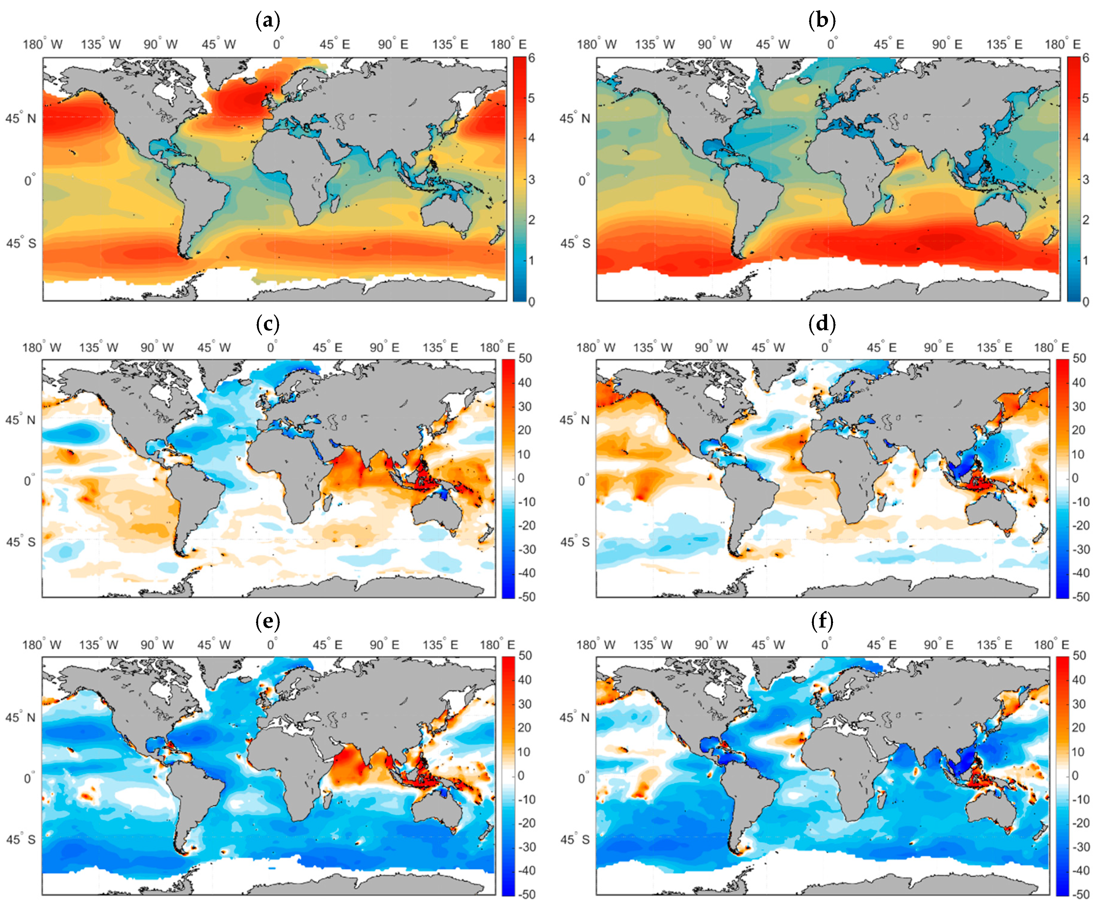
A similar comparison was done for the global DJF and JJA mean $H_s$ 95% percentiles, as shown in Figure 3. The comparison with ERA-Interim extreme wave heights showed lower relative differences compared to the seasonal $H_s$ means, with marginal or zero differences or patches of low over- and underestimations (less than 5%). The exceptions were in the North Atlantic, where the ensemble underestimated the 95% percentile wave heights by around 5–10% in DJF, and overestimated them along the trade-winds path in JJA, in the Arabian Sea and Bay of Bengal in DJF, and in the Solomon Sea in both seasons, where extreme wave heights were, in this case, overestimated by around 15% or more. On the other hand, the comparison between the seasonal PC20-E and CFSR mean $H_s$ 95% percentiles showed, for both seasons, a generalised underestimation of PC20-E (around 10% or less), with higher differences along the extratropical storm tracks, where the underestimation was of the order of 15% or even higher. The exceptions were, once more, the Arabian Sea and the Bay of Bengal in DJF, and the Solomon Sea in both seasons, where the 95% percentile wave heights were overestimated by the PC20-E compared to the CFSR by 10–15% or more.

Figure 4 displays the DJF and JJA mean $T_m$ relative differences between the global PC20-E and ERA-Interim (only). As with wave heights, the ensemble overestimated the mean wave periods, although less: globally, around 5% or less in DJF, with slightly higher values in the equatorial regions (more in the Pacific Ocean) and in the Arabian Sea (but still within the 10% range), with similar behavior in JJA, although with higher overestimations in the North Pacific (about 5–10%). In DJF, in the North Atlantic, the mean $T_m$ showed almost no differences compared to the ERA-Interim values, and in JJA, the overestimation was also rather low.

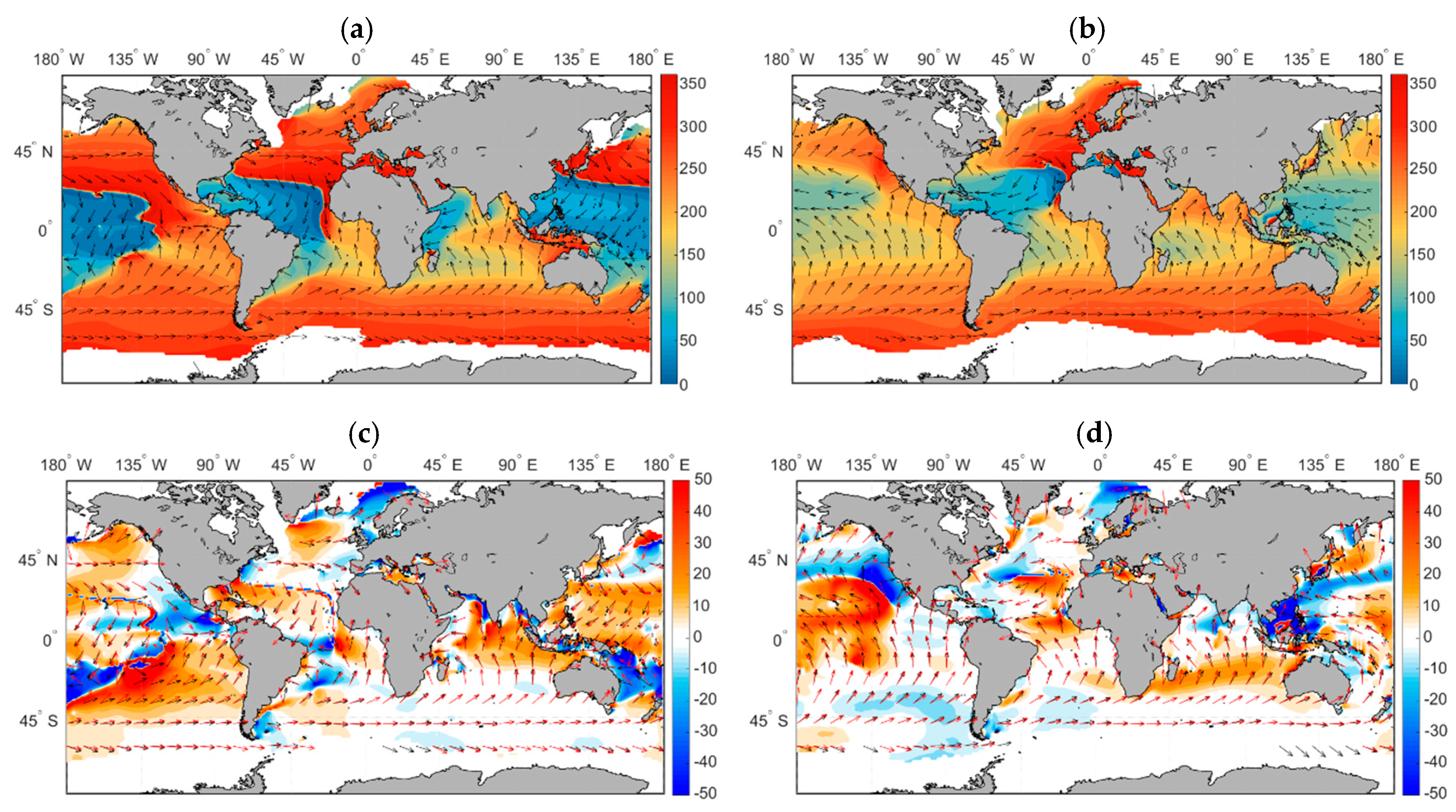
The differences between the global PC20-E and ERA-Interim DJF and JJA mean ${\theta }_m$ are presented in Figure 5. The seasonal differences are presented in the background contour, and the ERA-Interim mean DJF and JJA ${\theta }_m$ are also presented with arrows of different colors. Most differences were either negligible or close to zero, or between −10° (anti-clockwise) and 10° (clockwise) in both seasons. Some higher differences (about −20° to 20°) can be seen in the west tropical Pacific Ocean, in the Arabian Sea and Bay of Bengal, and east of Australia in DJF, and in the mid-latitudinal east North Pacific, in the South China Sea, and at high latitudes, as in the Barents Sea, in JJA. As with the seasonal $H_s$ and $T_m$, the ${\theta }_m$ comparisons with ERA-Interim were better in the North Atlantic sub-basin.

Despite some differences to ERA-Interim and CFSR, at this stage, it can be said that the agreement between PC20-E and the reanalyzed DJF and JJA mean and extreme wave heights, mean wave periods, and mean wave directions can be considered as relatively good. These differences were lower or in agreement with previous recent studies by [30,32,33,45]. Nevertheless, it is important to reason and understand what, to a certain extent, might be behind these differences. Firstly, part of the $H_s$ differences between PC20-E and the reanalysis, mostly in the equatorial Pacific Ocean, have to do with different land masks used in WAM C4.5.3 set-up in PC20 and in the reanalysis. Additionally, WAM C4.5.3 was proven to not properly damp swell in the light-wind intertropical areas, which can sometimes lead to an overestimation of the wave heights compared to the WAM version used in ERA-Interim and to the WW3 model used in CFSR. Some differences might also occur due to unresolved sub-grid scale bathymetry, which was taken into account in the ERA-Interim WAM version and in WW3, but not in the WAM C4.5.3 version used in the ensemble.

Table 2. Summary of PC20-E relative differences to the reanalysis. Percentages of global ocean area with as a function of global wave height ($H_s$), wave period ($T_m$), and wave direction (${\theta }_m$) relative differences. DJF—December to February; JJA—June to August; CFSR—Climate Forecast System Reanalysis; ERA-I—ERA-Interim.

	PC20-E DJF Differences (ERA-I/CFSR)			PC20-E JJA Differences (ERA-I/CFSR)
	$\%\mathbf{Area}\mathbf{with}\mathbf{Error}<\left|5\mathit{\%}/°\right|$	$\%\mathbf{Area}\mathbf{with}\mathbf{Error}\left|5-10\mathit{\%}/°\right|$	$\%\mathbf{Area}\mathbf{with}\mathbf{Error}>\left|10\mathit{\%}/°\right|$	$\%\mathbf{Area}\mathbf{with}\mathbf{Error}<\left|5\mathit{\%}/°\right|$	$\%\mathbf{Area}\mathbf{with}\mathbf{Error}\left|5-10\mathit{\%}/°\right|$	$\%\mathbf{Area}\mathbf{with}\mathbf{Error}>\left|10\mathit{\%}/°\right|$
$H_s$	16.99/31.82	50.27/52.48	32.74/15.70	35.03/20.36	42.39/57.87	22.58/21.77
$T_m$	25.12	66.38	8.50	44.67	41.40	13.93
${\theta }_m$	40.80	36.25	22.95	48.94	33.11	17.95

shows a summary of the PC20-E relative differences against the reanalysis. About 67% (84%) of the PC20-E $H_s$ global ocean field had relative errors lower than ±10% in DJF compared with ERA-Interim (CFSR). That area became about 77% for the comparison with both sets of reanalysis in JJA. Only about 32% (15%) or 22% (21%) of the PC20-E $H_s$ global ocean field in DJF had relative errors higher than ±10%. The PC20-E $T_m$ global scores are similar, with more than 91% (86%) of the global ocean area with errors lower than ±10% compared to ERA-Interim in DJA (JJA). The ensemble also represented ${\theta }_m$ well compared to ERA-Interim, with more than 76% (82%) of the ocean area with errors below ±10°.

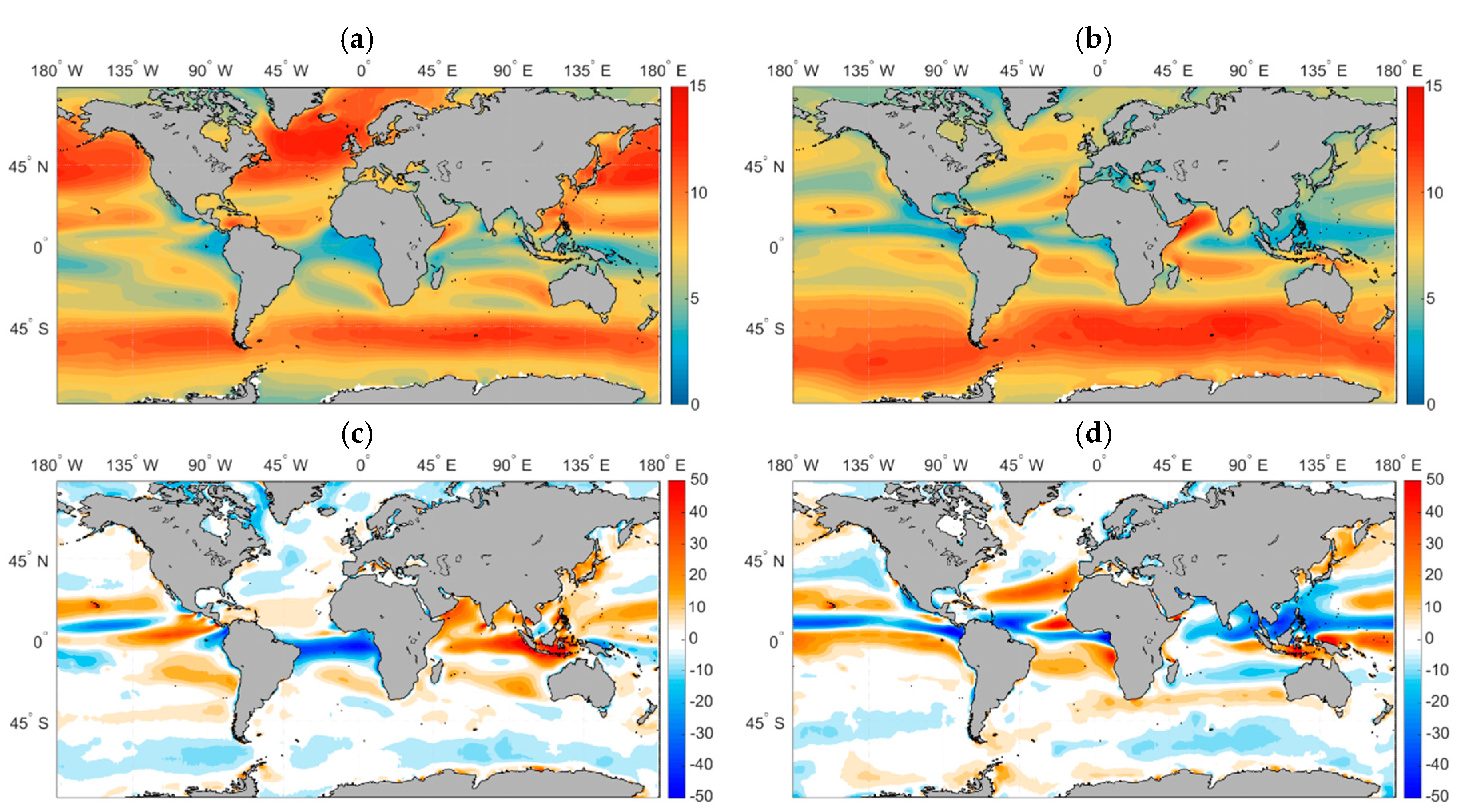
In search of additional justification for the differences shown in Figure 2, Figure 3, Figure 4 and Figure 5, the PC20-E and ERA-Interim DJF and JJA mean $U_{10}$ relative differences were computed for the basic wave parameters. As can be seen in Figure 6, the $U_{10}$ differences were strikingly low (less than 5%) or close to zero in most of the global ocean, particularly in the extratropical areas in both hemispheres. These differences were lower that the $H_s$ ones shown in Figure 2. The relative differences were higher in the intertropical latitudes, where the mean $U_{10}$ absolute magnitudes (and respective anomalies) were actually low. These differences, most pronounced in the equatorial areas, can be attributed to differences in the placement of the intertropical convergence zone (ITCZ) in EC-Earth, particularly in the Atlantic Ocean [46], since slight meridional differences can lead to substantial relative differences in the wind speed there. Nevertheless, as with the mean basic wave parameters, the PC20-E and the reanalyzed DJF and JJA $U_{10}$ differences can be seen as relatively low. The PC20-E relative $H_s$and $T_m$ differences in the Arabian Sea can be explained by the ensemble $U_{10}$ differences compared to ERA-Interim.

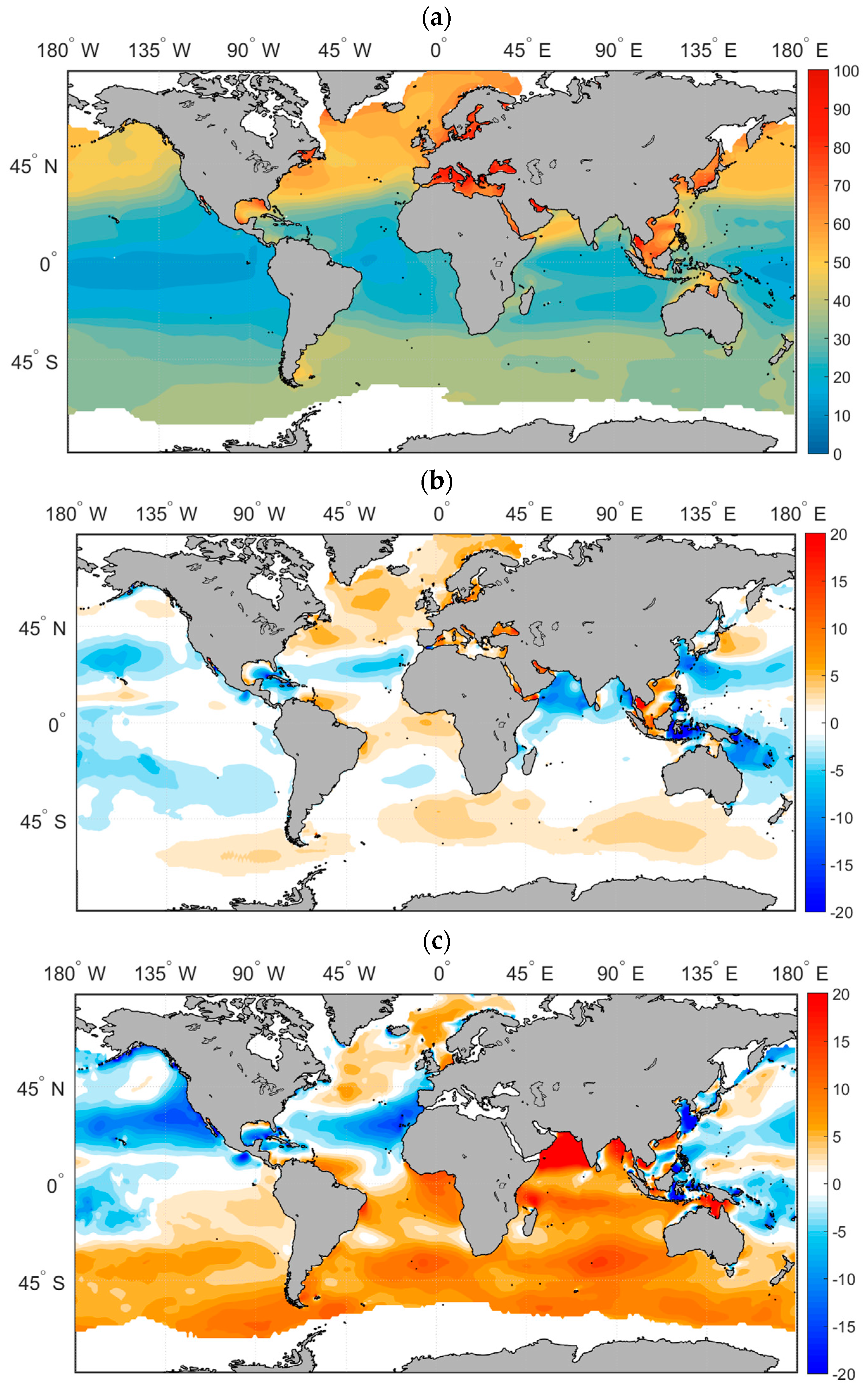
Figure 7 depicts the ensemble’s ability to reproduce the $H_s$ annual variability, as measured by the MAV (Equation (3)), in comparison with the reanalysis. Here, the comparisons are presented as anomalies (PC20-E minus reanalysis MAVs: $MA{V}_{PC20-E}-MA{V}_R$), and not as relative differences. The North Pacific and North Atlantic sub-basins, where the inter-seasonal wave height variability is highest [1,3,7] had the highest MAV values (50–60%), followed by the southern hemisphere extratropical storm paths (30–40%), not counting marginal sea areas. Compared to ERA-Interim, the PC20-E MAV showed small differences: marginal or inexistent, or between −5% (in the lower latitudes) and 5% (in the North Atlantic and southern hemisphere extratropical latitudes). When compared to CFSR, the differences were considerably higher (about −10% to 10%), particularly in the southern hemisphere extratropical latitudes. These differences might be related to the different temporal resolutions (6 h in PC20-E and ERA-Interim, and 3 h in CFSR), since CFSR is known to better simulate extreme wave heights compared to ERA-Interim [72]; however, it also to slightly overestimates $H_s$. These differences in the PC20-E MAV compared to the CFSR were higher in the Arabian Sea (close to 20%).

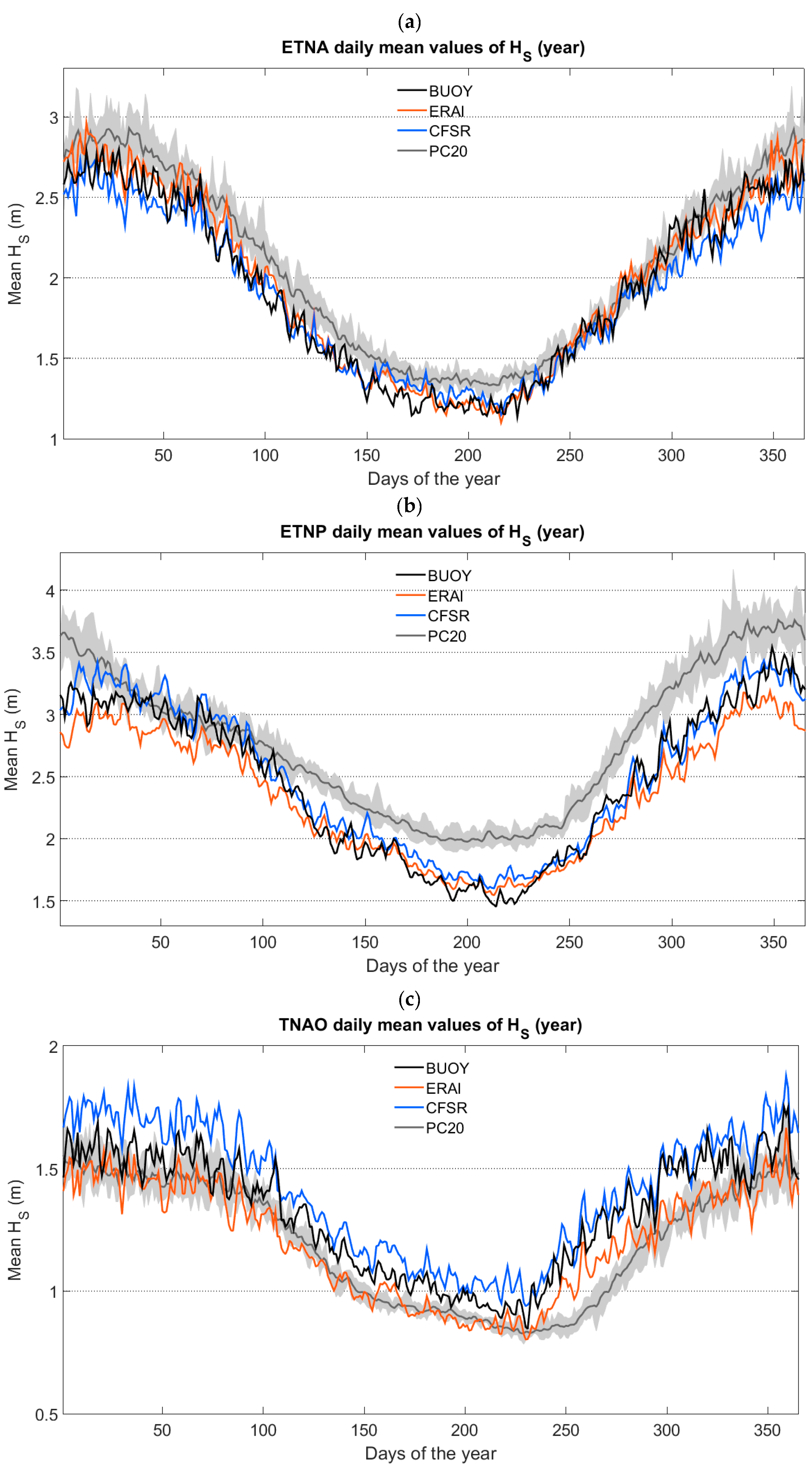
The PC20-E intra-annual variability was also evaluated through comparison with in situ $H_s$ observations (positions in Figure 1). For that matter, the comparisons were done separately for three of the regional areas shown in Figure 1: extratropical North Pacific (ETNP), extratropical North Atlantic (ETNA), and tropical North Atlantic (TNAO). The only buoy in the tropical eastern North Pacific (TENP) area was included in the ETNP for convenience. The collocated (at the in situ measurements positions) daily averaged $H_s$ observations for PC20-E, ERA-Interim, and CFSR (averaged in each of the three areas) plotted in a Julian year are shown in Figure 8. The length of the PC20 time series was matched with the observational records following [78] methodology, as described in Section 2. In the background, the spread of the ensemble members is also shown as a grey band. Despite some discrepancies, the intra-annual variability was well captured by the ensemble in the three areas. In the ETNA, the agreement was better, with a slight overestimation (less than 0.1 m). During the last months of the year (from day 250 onwards, i.e., from September to December), when wave heights start to increase in the North Atlantic, the agreement between the PC20-E, the observations, and the reanalysis was close to ideal. This agreement was not as good in the ETNP, where the $H_s$ spread between observations and reanalysis was also higher. On the other hand, in the first months of the year (mostly form mid-January to April) the agreement was good in that area; however, from there onwards, PC20-E overestimated wave heights by about 0.2 m. This overestimation, as mentioned before, can be explained, to a great extent, by the differences in the land mask used in the climate simulations, with greatest differences in the equatorial Pacific Ocean. For that reason, waves generated in the South Pacific Ocean propagate more freely as swell, less damped, into the North Pacific sub-basin, leading to this slight overestimation of wave heights in the PC20-E, mostly during the second half of the year. In the TNAO area, with in situ observations mostly concentrated in the Gulf of Mexico and the Caribbean Sea where swell penetration is lower, the agreement between PC20-E and the observations and reanalysis was good for most of the year. There was, nevertheless, some underestimation during the tropical cyclone season that can be linked to an underestimation of the wind speeds in JJA in that area, as shown in Figure 6d.

The relatively low variability between the ensemble members in Figure 8 (shown in the back as a grey band around the ensemble mean) can now be seen at a global scale in Figure 9, where the PC20-E inconsistency (for $H_s$ and $T_m$; absolute pairwise difference between the ensemble members PC20-1 to PC20-7) is shown. The $H_s$ inconsistency was relatively small: about 0.1 m or less in the extratropical and high latitudes in DJA (only in the southern hemisphere in JJA), and less than half of that value in the intertropical latitudes and marginal seas in both seasons. The PC20-E $T_m$ inconsistency was slightly higher than that of the $H_s$, or at least more evenly distributed in the global ocean, with values lower than 0.1 s. The highest values can be found toward the eastern oceanic margins and in the northern sector of the Indian Ocean in DJF, and also in the western South Atlantic in JJA. The intra-ensemble variability, as seen from these values, was, therefore, low as a result of the single GCM-forcing strategy, and it was certainly lower than in the multi-forcing ensemble in the article by [43].

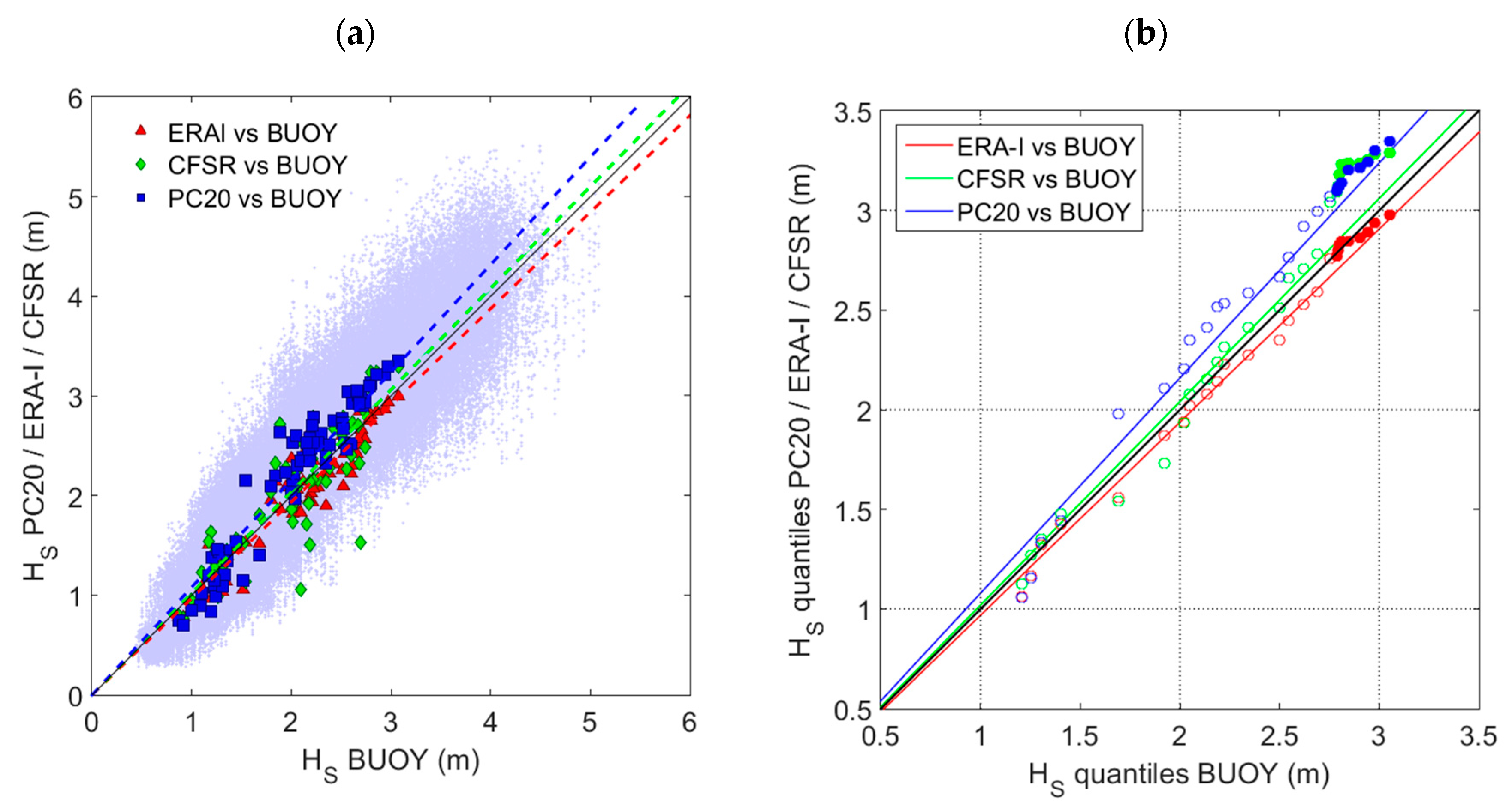
The scatter plot in Figure 10 compares the ensemble with the in situ $H_s$ observations. As in Figure 7, the ERA-Interim and CFSR collocated wave heights are also included. The length of the PC20-E time series was once again matched with the observational records following the methodology in [78]. A quantile–quantile (Q–Q) plot is also included in Figure 10, with collocated PC-20-E, in situ observations, and reanalysis. An overestimation of the ensemble’s highest wave heights can be seen in the scatter plot compared to the three datasets. Lower wave heights were, on the other hand, slightly underestimated. The overestimation was mostly due to the overestimation in the North Pacific, and it was hardly present if the comparison was made only for the North Atlantic observations (not shown). It is worthy of note that the CFSR wave heights were closer to the observations, slightly overestimating them, while the ERA-Interim underestimated $H_s$ (in agreement with [72]). A similar behavior can be seen in the Q–Q plot, with PC20-E underestimating the lower quantile wave heights, while consistently overestimating them in the higher-order ones, particularly the extreme wave heights. It is also worthy to note the pronounced overestimation of extreme wave heights in the CFSR hindcast compared to the observations. A summary of statistics of the PC20-E $H_s$ comparison against the observations and reanalysis at the observational positions is presented in

Table 3. Summary statistics of PC20-E, Era-Interim, and CFSR $H_s$ comparisons against in situ measurements. RMSE—root-mean-square error.

	Bias (m)	RMSE (m)	r
PC20-E vs. Observations	0.16	0.39	0.93
PC20-E vs. ERA-I	0.22	0.40	0.94
PC20-E vs. CFSR	0.12	0.46	0.88

. The high correlation coefficients between PC20 and the observations and reanalysis (consistently higher than 0.93 for the observations and ERA-Interim, and 0.88 for the CFSR) confirm the good scores of PC20-E, despite the generalized overestimation of wave heights at these positions.

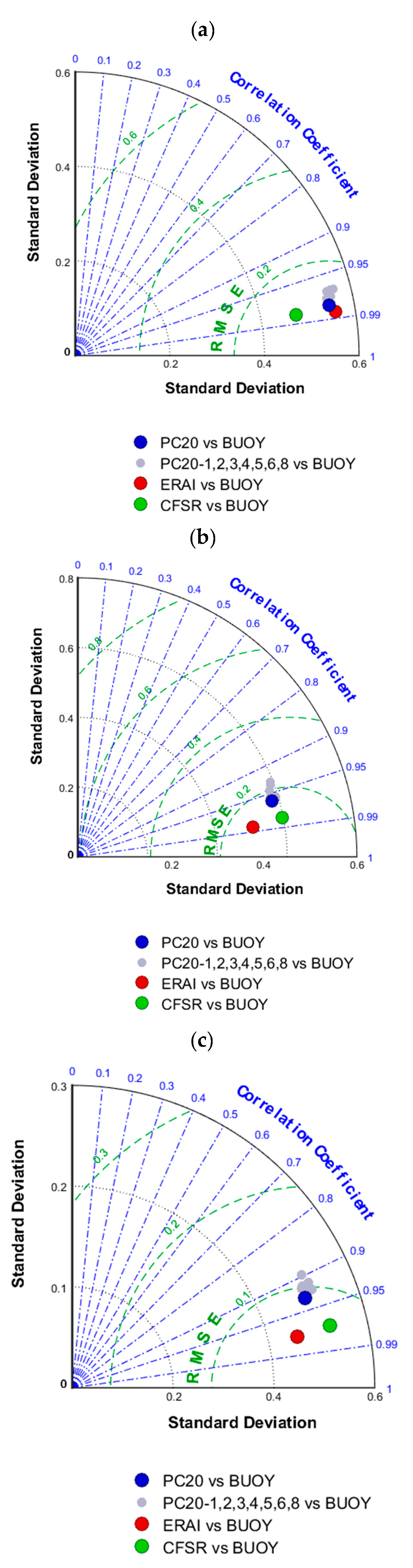
Taylor diagrams of the comparison between PC20-E and observations, separately for the ETNP, ETNA, and TNAO areas, are shown in Figure 11. The comparison between each of the ensemble members (PC20-1 to PC20-7) and observations, as well as similar comparisons for ERA-Interim and CFSR, are also presented. The PC20-E showed better results (higher correlation coefficient and lower RMSE) than any individual ensemble members. The variability, as represented by the standard deviation, was similar between PC20-E and the ensemble members, and closer to the reanalysis. The correlation between PC20-E and the observations was highest in the ETNA, and lowest in the TNAO, despite the fact that the RMSE was lowest in the Caribbean and Gulf of Mexico compared to the other two areas. In the TNAO, the PC20 scores were also more detached from those of the reanalysis.

The intra-annual variability of the PC20-E mean spatial bias (Equation (1)) and mean normalized differences (spatially averaged) from the comparison with ERA-Interim and CFSR (daily means shown in a Julian year) is presented in Figure 12 for each of the 13 regional areas, as well as for the global ocean. The ensemble’s overestimation compared with ERA-Interim is clear, as shown in the previous Figures, with a bias on the order of 0.2 and 0.25 m, slightly higher during the last quarter of the year. This overestimation toward ERA-Interim (from 9 to 11%, also higher in the last quarter of the year), is also clear in the global normalized differences. The global agreement of the PC20-E with CFSR was considerably higher, with lower biases (from −0.1 to 0.15 m, and most of the year close to zero) and also lower normalized differences (between −2% to 4%, but lower for most of the year). When looking at the regional areas, the lowest biases and normalized differences in comparison with ERA-Interim occurred in the extratropical areas, particularly in the ETNA, extratropical South Atlantic (ETSA), and extratropical South Indian (ETSI) areas. The highest differences occurred in the Pacific Ocean intertropical regions. The same occurred, with lower differences, for the comparison with CFSR. Nevertheless, the CFSR comparison displayed a higher bias and relative difference in the tropical North Indian (TNIO).

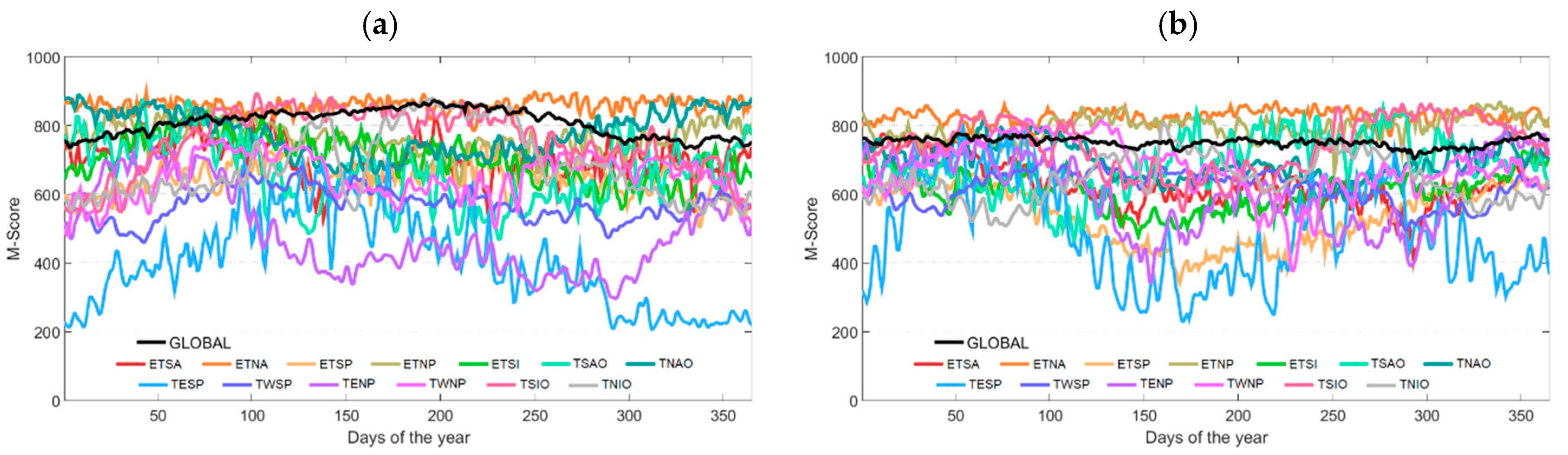
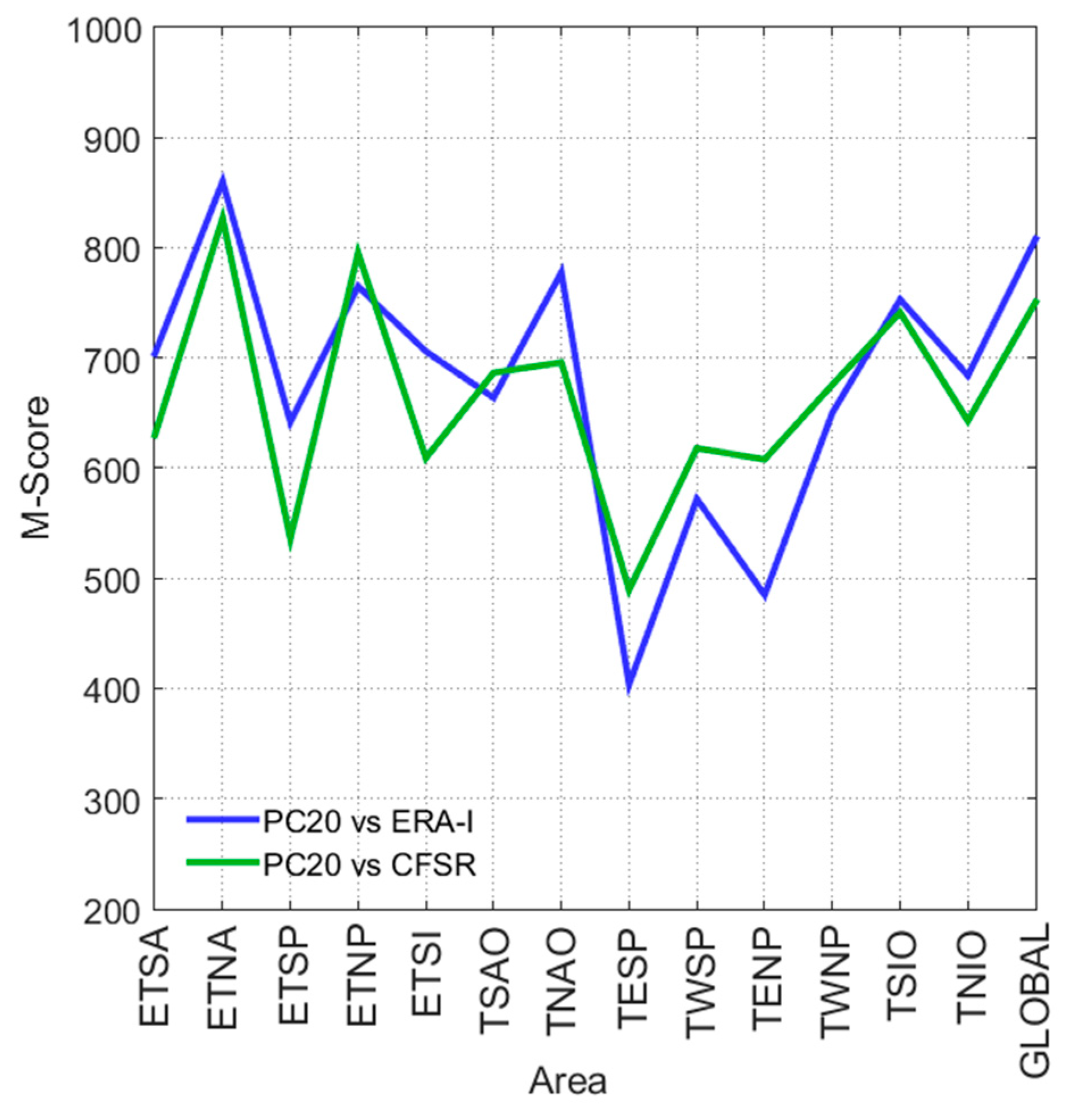
The intra-annual variability of the averaged PC20-E M-Scores (Equation (4)) was also computed globally and for each of the 13 regional areas, as shown in Figure 13. The highest M-Score values can be found in the ETNA area for the comparison with ERA-Interim (with an annual average of 860; see

Table 4. Summary of regional and global M-Scores. ETNP—extratropical North Pacific; TENP—tropical eastern North Pacific; TWNP—tropical western North Pacific; TWSP—tropical western South Pacific, TESP—tropical eastern South Pacific, ETSP—extratropical South Pacific; ETNA—extratropical North Atlantic; TNAO—tropical North Atlantic; TSAO—tropical South Atlantic; ETSA—extratropical South Atlantic; TNIO—tropical North Indian; TSIO—tropical South Indian; ETSI—extratropical South Indian.

	PC20 vs. ERA-I			PC20 vs. CFSR
	Annual	DJF	JJA	Annual	DJF	JJA
ETSA	704	714	691	630	713	611
ETNA	860	861	858	827	824	834
ETSP	642	601	659	536	628	428
ETNP	765	798	730	796	792	792
ETSI	706	708	714	609	658	551
TSAO	664	738	597	687	669	739
TNAO	778	851	715	696	726	662
TESP	404	298	483	490	509	382
TWSP	572	540	592	618	597	648
TENP	485	613	418	608	720	547
TWNP	650	597	608	676	669	612
TSIO	753	634	825	741	757	651
TNIO	684	591	808	643	600	681
Global	808	768	853	751	760	750

for mean M-Score values). Similar values can be found for the comparison with CFSR, consistently higher than 820 (annual average of 827). The M-score values for the remaining extratropical areas can also be classified as high, particularly during the respective winter season) for the comparison with ERA-Interim: consistently higher than 700, with the exception of the extratropical South Pacific (ETSP) area. These scores were similar for the comparison with CFSR, although with lower (higher) scores in the ETSA, ETSP, and ETSI (ETNP)—see Table 4. In the intertropical areas, the M-Scores were still high, with mean values of 778 (696) and 664 (687) in the TNAO and TSAO, respectively, for the ERA-Interim (CFSR) comparison. These values decreased in the intertropical Pacific and Indian Ocean areas, for both comparisons, with the lowest M-score values occurring in the tropical eastern South Pacific (TESP) area. Globally, the M-Scores were comparable for both sets of reanalysis (consistently higher than 750), with annual means of 808 and 751 for the comparisons with ERA-Interim and CFSR, respectively. These M-Score values were comparable to or higher than the ones shown in the article by [43], and onsistent with the ones shown for atmospheric CMIP5 GCM evaluations in the article by [80], showing the relative high skill of PC20. Additional information can be seen in Table 4 and Figure 14, where a graphic display of regional and global M-Scores can be seen simultaneously.

Figure 15 displays the box plots for the $H_s$ annual M-scores between the PC20-E and the reanalysis, globally and for each or the 13 regional areas. The respective annual and seasonal (DJF and JJA) means are also plotted. As a measurement of the intra-annual variability of the regional and global M-score, the inter-quartile range (IQR) was lower in the extratropical areas in the comparison with ERA-Interim, particularly in the ETNA and ETNP, where the differences between the lower and higher extremes were also lower, particularly in the ETNA area. While the same occurred in the northern hemisphere extratropical areas, regarding the CFSR comparison, it was not exactly the same for the southern hemisphere, particularly in the ETSP. The highest IQR (intra-annual variability) can be seen in the TESP area (which also had the lowest annual and seasonal M-score means) for both sets of reanalysis. In Figure 13, it can be seen that the M-scores were comparable in terms of magnitude and variability, particularly in the extratropical areas. It is interesting to note that, while the mean M-regional scores for the extratropical areas were higher in the comparison with ERA-Interim (735, 737, and 730, for the annual, DJF, and JJA means, respectively), the situation somehow reversed in the intertropical areas when compared to CFSR (680, 723, and 643, respectively).

4. Summary and Conclusions

The performance skills of a single-forcing (EC-Earth), single-wave model (WAM), and single-scenario (RCP8.5) dynamic wave climate ensemble in reproducing the present time wave climate (as represented by the historic period) were presented. The ensemble was designed with the goal of reducing the variability inherent in using a multi-forcing GCM approach to force the same wave model. The PC20-E ensemble’s historic period (1979–2005) was extensively compared against a set of 72 in situ wave-height observations, as well as to the ERA-Interim reanalysis [49] and CFSR hindcast [50].

It was shown that the differences between the ensemble and the reanalyzed DJF and JJA mean and extreme $H_s$, mean $T_m$, and mean ${\theta }_m$ can be considered as relatively low, in line with (or lower than) previous global wave climate studies. The PC20-E comparison with the 72 in situ $H_s$ observations showed a good agreement, with small biases and high correlation coefficients, as well as a good representation of the intra-annual variability. Nevertheless, the ensemble had a tendency to overestimate (underestimate) the mean wave heights, in both seasons, compared to ERA-Interim (CFSR). The agreement with ERA-Interim was better in the North Atlantic, and with CFSR in the North Pacific. The comparison with the reanalysis was weaker in the Arabian Sea. Apparently, EC-Earth has some difficulties in resolving the South Asian Monsoon. Nevertheless, most probably due to resolution, ERA-Interim winds already had problems in that area, as shown by [81,82]; hence, a dedicated study for this area would be needed. The PC20-E overestimation of extreme wave heights was lower; in fact, compared to ERA-Interim, the ensemble had almost equal areas of over- and underestimation in both seasons. Compared to CFSR, the ensemble extreme $H_s$ seasonal fields were underestimated almost across the entire global ocean. It was shown that ERA-Interim underestimates extreme wave heights, while CFSR has a tendency to overestimate them [72]. Figure 16 shows the mean ERA-Interim and CFSR inconsistency (mean absolute pairwise difference). As can be seen, the differences between the reanalysis and the hindcast can reach values of 0.7–0.8 m in the Southern Ocean storm belt during the austral winter, and values on the order of 0.6–0.7 m in the extratropical latitudes of both hemispheres in DJF. These differences are mostly due to the overestimation (underestimation) of the CFSR (ERA-Interim) wave heights. It would be tempting to state that, with the PC20-E $H_s$ seasonal fields somewhere in between, they are closer to reality. Nevertheless, without a third global wave dataset and further investigation, that cannot be concluded. The ensemble comparison with the ERA-Interim mean $T_m$ seasonal fields also revealed some overestimation; however, it was lower than that seen for the mean seasonal wave heights.

At a regional level, the PC20-E $H_s$ had a rather good performance in the extratropical areas of both hemispheres, particularly in the North Atlantic sub-basin, with low biases and relative differences during most of the year, especially compared to the CFSR. These skills were lower in the areas along the equatorial Pacific Ocean. Globally, the inter-annual variability of the biases from the ERA-Interim and CFSR comparisons showed values between 0.2 and 0.28 m, and −0.1 and 0.1 m, respectively. To a certain extent, a similar situation occurred for the PC20-E regional and global M-Scores, i.e., higher M-Scores in the extratropical areas (in this situation, slightly higher for the comparison with ERA-Interim than with CFSR), and lower in the tropical areas, particularly in the Pacific Ocean, in line with the multi-forcing ensemble of [43].

The agreements between the $H_s$, $T_m$, and ${\theta }_m$ PC20-E and reanalysis, and between PC20-E and the in situ $H_s$ observations show that the WAM model, forced by the EC-Earth winds and SIC, produces considerably realistic results of the global wave climate at the end of the twentieth century wave climate. These results give a good degree of confidence in the ability of the ensemble to simulate a realistic climate change signal. Future research on the impact of climate warming on future wave climate, using the single-forcing, single-model, and single-scenario dynamic wave climate ensemble is to be conducted following the present study, including the impact on wave power, and on the wind sea and swell patterns.