Model Uncertainties for Soil-Structure Interaction in Offshore Wind Turbine Monopile Foundations

Abstract

Monopiles are the most common type of foundation used for bottom-fixed offshore wind turbines. This investigation concerns the influence of uncertainty related to soil–structure interaction models used to represent monopile–soil systems. The system response is studied for a severe sea state. Three wave-load cases are considered: (i) irregular waves assuming linearity; (ii) highly nonlinear waves that are merged into the irregular wave train; (iii) slamming loads that are included for the nonlinear waves. The extreme response and Fourier amplitude spectra for external moments and mudline bending moments are compared for these load cases where a simpler static pile-cap stiffness and a lumped-parameter model (LPM) are both considered. The fundamental frequency response of the system is well represented by the static pile-cap stiffness model; however, the influence of higher modes (i.e., the second and third modes with frequencies of about 1 Hz and 2 Hz, respectively) is significantly overestimated with the static model compared to the LPM. In the analyzed case, the differences in the higher modes are especially pronounced when slamming loads are not present.

1. Introduction

In the design of offshore wind turbines, one is required to consider a very large number of load cases; this emphasizes the need for computational efficiency and accuracy. For bottom-supported offshore wind turbines, to improve the efficiency of time-domain simulations, various modeling approaches have been attempted (reviewed in the paper by Damgaard et al. [1]) that seek to include only a few degrees of freedom for the foundation in the overall turbine–tower–foundation system. Direct insight into the pile behavior without the necessity of back-calculating the pile response can be achieved by using p–y curves and a Winkler-type model for the soil–pile interaction. This approach has been used widely in the literature and by industry for static as well as cyclic and dynamic analysis of monopiles [2,3,4,5,6]. For detailed analysis of the pile and soil behavior, three-dimensional numerical models have also been applied [7,8].

However, for fully coupled dynamic analyses in which the entire system of equations for the foundation and the turbine are integrated into the aeroelastic simulation code, cone models [9] or lumped-parameter models (LPMs) [10,11] can be very useful. Such models only introduce a few degrees of freedom in addition to those present in the computational model of the turbine and its support structure. The use of an LPM comes at the cost of requiring back-calculation of the pile response; but this is equivalent to the back-calculation that is necessary in order to extract cross-sectional forces and stresses in other parts of the system, e.g., the blades or the tower. Hence, this study concerns a simplified model of an offshore wind turbine (OWT) on a monopile, focusing on the model uncertainty related to inaccurate treatment of the dynamic soil–structure interaction.

The tubular tower and support structure are modeled by two-node, plane beam finite elements using cubic Hermitian weight functions and accounting for shear flexibility in accordance with Timoshenko beam theory [12]. Distributed rigid masses are placed at the top of the structure to model the nacelle, hub and rotor, at the top of the support structure to model the boat landing, and at the waterline to model the transition piece. The submerged part of the structure is loaded by waves, and the bottom part is embedded in the seabed as described in the following sections. The wind loads are disregarded based on the assumption that they are significantly smaller than the wave loads in an ultimate limit state when the blades are pitched out of the wind. Further, no aerodynamic or hydrodynamic damping is considered.

2. Wave Loads

Compared to the motion of the water during wave action in extreme conditions, the displacement of the pile is assumed to be negligible. Hence, one-way coupling between the submerged pile and the surrounding water can be assumed without significant loss of accuracy.

2.1. Load Model for Vertical Surface Piercing Circular Cylinders

Wave loads on cylindrical structures involve inertia and drag loads, usually calculated by the Morison equation [13] which, for circular vertical piles of radius $R_{\mathrm{p}}$, gives the horizontal force per unit length as:

$$f\left(z,t\right)=\pi {\rho }_{\mathrm{w}}{C}_{\mathrm{M}}{R}_{\mathrm{p}}^2\dot{v}\left(0,z,t\right)+{\rho }_{\mathrm{w}}{C}_{\mathrm{D}}{R}_{\mathrm{p}}v\left(0,z,t\right)\left|v\left(0,z,t\right)\right|.$$

(1)

Here, the first term is the inertia load, and the second term is the drag load. Further, $v\left(x,z,t\right)$ and $\dot{v}\left(x,z,t\right)$ are the horizontal water particle velocity and acceleration, respectively. These are evaluated at the center of the pile (at $x=0$) at elevation $z$ and calculated by the wave theories given below. The inertia and drag coefficients used are $C_{\mathrm{M}}=1.62$ and $C_{\mathrm{D}}=1.44$, estimated from [14] based on roughness due to marine growth of 0.05 m. Thus, the wave load is drag-dominated. The density of seawater is ${\rho }_{\mathrm{w}}=1020$ kg/m³, and the pile radius employed in the present study is $R_{\mathrm{p}}=3$ m. This radius is significantly smaller than the wavelengths resulting from the models considered below, which justifies use of the Morison equation.

A surface-piercing structure (as is the case with the one concerned in this study) is subjected to slamming loads that might be a significant load contribution in breaking or highly nonlinear waves. These forces per unit length are computed as:

$$f_{\mathrm{I}}\left(z,t\right)={\rho }_{\mathrm{w}}{C}_{\mathrm{s}}{R}_{\mathrm{p}}v\left(-R_{\mathrm{p}},z,t\right)\left|v\left(-R_{\mathrm{p}},z,t\right)\right|.$$

(2)

These loads act in the upper part of the wave and might be very important for the structural response, as the load may be high and of much shorter duration than the drag and inertia loads. In the present case, the slamming coefficient for non-breaking or spilling waves on vertical cylinders given by DNV RP-OS-J101 [14] is used:

$$C_{\mathrm{s}}\left(s\right)=5.15\left(\frac{2R_{\mathrm{p}}}{2R_{\mathrm{p}}+19s}+\frac{0.107s}{2R_{\mathrm{p}}}\right)\mathrm{for}0\le s\le 2R_{\mathrm{p}},$$

(3)

where $s$ is the penetration distance, i.e., the horizontal distance from the periphery on the wet side of the cylinder to the sloping water surface for the section in question, measured in the direction of the wave propagation.

The DNV formulae for the slamming load and coefficient are based on the assumption of constant particle velocity $v$ (during penetration by the cylinder section of the sloping water surface), which is in fact not the case in waves. In the present study, the particle velocity used in Equation (2) is taken at the pile front $v\left(-R_{\mathrm{p}}, z,t\right)$ based on the wave theories described below, which should lead to a reasonable prediction of the slamming load.

The total forces may be calculated by numerical integration of the above-defined distributed Morison and slamming loads from the mudline to the sea surface elevation. For simplicity, it shall be assumed that the pressure variation with time does not propagate into the seabed. To calculate the loads to be applied within the finite-element (FE) model, the load acting on an element is divided into nodal forces in such a way that both the instantaneous quasi-static shear force and bending moment are correct at all the nodes.

2.2. Linear and Nonlinear Wave Kinematics

Linear, irregular, unidirectional waves were generated based on a JONSWAP spectrum with a peak-enhancement factor of 3.3. Time series of the sea surface elevation were obtained by Inverse Fast Fourier Transformation using Rayleigh-distributed amplitudes and independent uniformly distributed (0, 2π) phases at each frequency. The particle velocities and accelerations were calculated in the frequency domain using linear transfer functions for 200 elevations from the seabed to the mean water level. Subsequently, inverse Fourier transforms were used to calculate the water particle velocity and acceleration time series at these 200 levels. These velocities and accelerations were stretched to the surface using Wheeler stretching [15] and then applied in the Morison equation.

Additionally, highly nonlinear regular waves were generated using the stream function theory of Rienecker and Fenton [16]. This is a universal theory valid for regular waves on a horizontal seabed when the stream-function order $N$ is chosen to be high enough. The order $N=20$ was found to be sufficient for the wave conditions in the present study.

2.3. Load Scenarios

Based on 50-year sea state conditions, three load scenarios are defined:

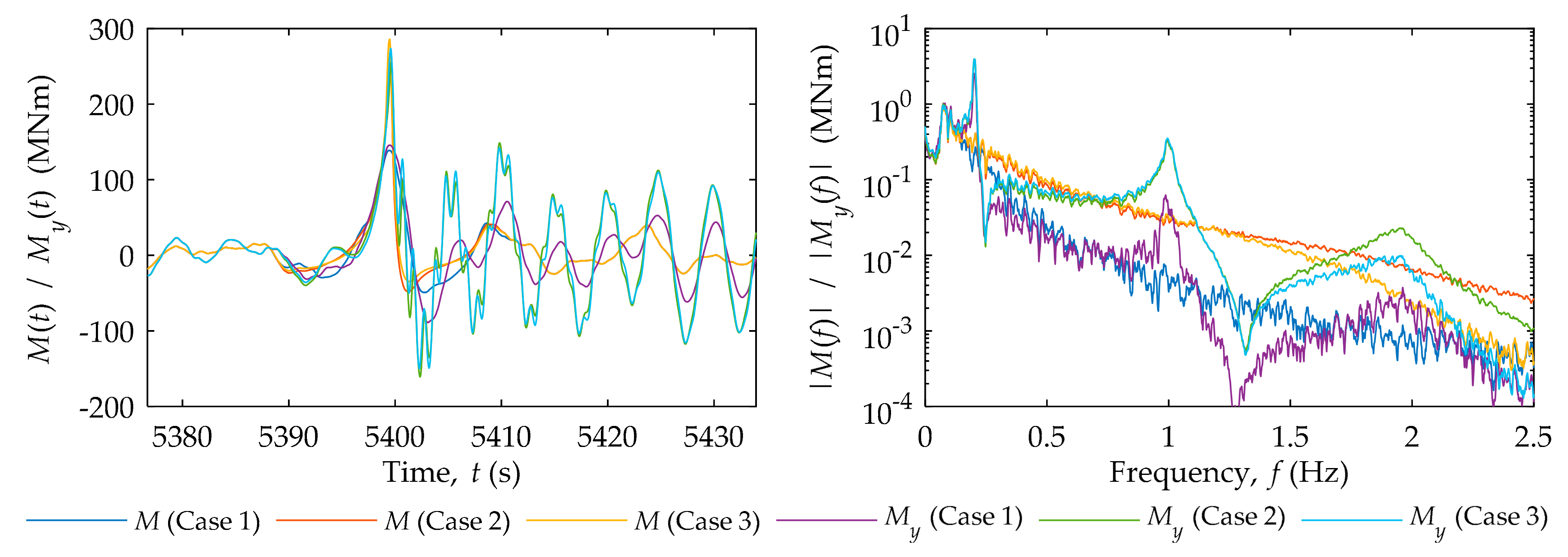
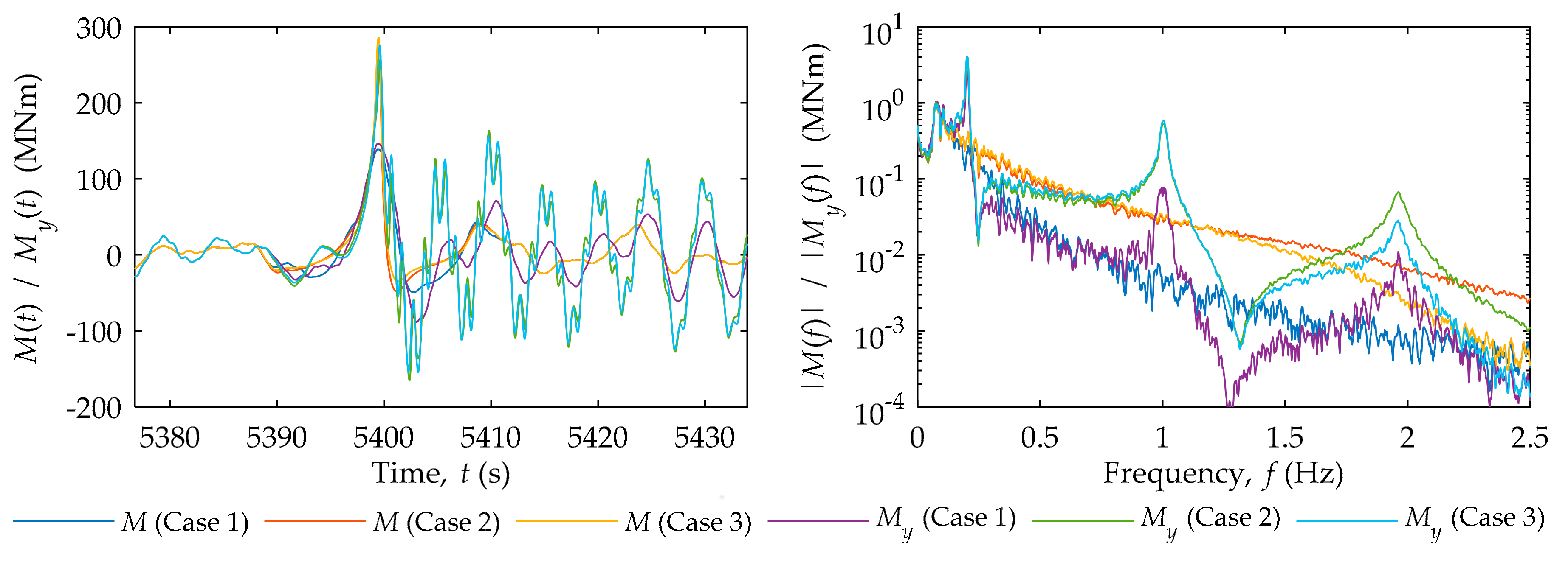
• Load Case 1: Linear irregular waves with significant wave height ${\mathrm{H}}_{\mathrm{m}0}=10$ m, peak wave period ${\mathrm{T}}_{\mathrm{p}}=13$ s. The duration of the simulated time series is 3 h corresponding to around 1000 waves. Loads are calculated by Morison’s equation without slamming contribution.
• Load Case 2: Same as Load Case 1 but where one wave in the irregular wave train is substituted by a stream function wave with $\mathrm{H}=18.7$ m, $\mathrm{T}=11.45$ s corresponding approximately to the maximum wave in the irregular series (Rayleigh distributed wave heights). This leads to a highly nonlinear wave that is merged into and out of the irregular wave by a cosine taper window. The regular wave is fully active for one wave period and merged in and out in half a period to either side.
• Load Case 3: Same as Load Case 2 but including slamming loads for the stream-function wave.

3. Lumped-Parameter Models for the Foundation

While the issues of uncertainty, derived system frequencies, and influence on long-term loads arising from relatively simple monopile foundation models commonly employed in practice have been addressed elsewhere [17,18], a lumped-parameter model of a monopile foundation is developed in three steps and used in the present study. The first step comprises rigorous modelling of the subsoil and coupling with an FE model of the pile. Second, the equivalent complex-valued dynamic stiffness of the pile cap is evaluated at a number of frequencies in the relevant frequency range. Third, a lumped-parameter model (LPM) is fitted to the dynamic response of the pile–subsoil system. This LPM is then assembled together with the model of the structure in order to allow time-domain analysis of the response due to the wave loading.

3.1. Semi-Analytical Model of Monopile Response in the Frequency Domain

In the present analysis, the seabed is modelled as a linear viscoelastic layered half-space. Even though the structural analysis is two-dimensional, a three-dimensional model of the soil is necessary to account for the spatial distribution of forces and radiation of waves. The solution is established in a horizontal wavenumber–frequency domain, assuming that all the layers consist of homogeneous material and that all the interfaces (including the mudline) are horizontal. A relationship can now be specified between the states of traction and displacements at the top and bottom of each layer:

$${\mathbf{S}}^{j,1}\left(k_x,k_y,\omega \right)={\mathbf{T}}^j\left(k_x,k_y,\omega \right){\mathbf{S}}^{j,0}\left(k_x,k_y,\omega \right),$$

(4a)

$${\mathbf{S}}^{j,m}\left(k_x,k_y,\omega \right)={\left\{{\widehat{u}}_x^{j,m},{\widehat{u}}_y^{j,m},{\widehat{u}}_z^{j,m},{\widehat{t}}_x^{j,m},{\widehat{t}}_y^{j,m},{\widehat{t}}_z^{j,m}\right\}}^T,m=1,2,\dots$$

(4b)

where ${\mathbf{S}}^{j,1}$ and ${\mathbf{S}}^{j,0}$ are the states evaluated at the top and bottom of layer j, respectively, and ${\mathbf{T}}^j$ is the layer transfer matrix evaluated in closed form in terms of the horizontal wavenumbers, $k_x$ and $k_y$, and the angular frequency, $\omega$. Furthermore, ${\widehat{u}}_x^{j,m}$, ${\widehat{u}}_y^{j,m}$ and ${\widehat{u}}_z^{j,m}$ are the displacement components, whereas ${\widehat{t}}_x^{j,m}$, ${\widehat{t}}_y^{j,m}$ and ${\widehat{t}}_z^{j,m}$ are the traction components in the horizontal wavenumber–frequency domain. As outlined by Andersen and Clausen [19], the transfer matrices ${\mathbf{T}}^j$ for the individual soil layers can be multiplied to obtain the transfer matrix for the stratum. Given that traction is applied in terms of axisymmetric distributed loads, Fourier transformation of the loads into the wavenumber domain can be done analytically. The displacement response at a receiver point somewhere inside the soil can be evaluated numerically along a single wavenumber axis. The inverse Fourier transformation applied to obtain the response in the space domain is semi-discrete as it only involves one-dimensional numerical integration. The remaining calculations can be done analytically, and the general solution for arbitrary relative positions of the source and receiver points can be determined by coordinate transformation.

The pile is modeled using the same beam FE formulation as the structure. To obtain realistic soil–structure interaction, coupling to the soil is defined over the perimeter of the pile and not along the beam axis. Full connectivity between the pile and the soil is assumed. Hence, the interior/exterior surfaces of the tubular monopile can be coupled to the same cylindrical surface within the soil. Assuming that the cross section at each node within the FE model of the pile behaves as a rigid ring, in compliance with beam kinematics, a dynamic stiffness matrix for the subsoil is determined for each angular frequency, $\omega ,$ as follows:

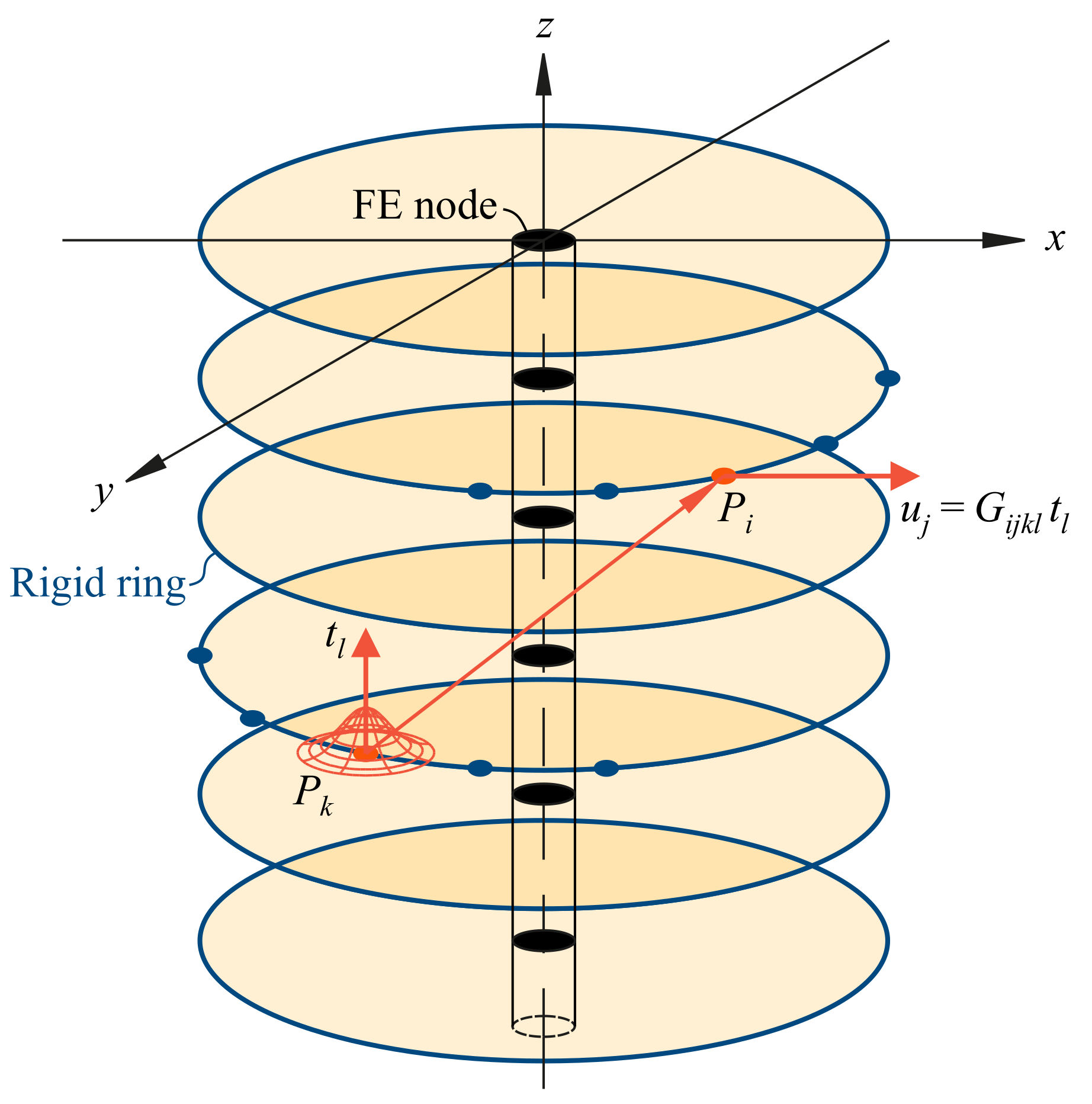
• The mid-surface of the monopile wall is discretized into a total of $n$ points, forming a ring with 18 points at the level of each FE node as illustrated in Figure 1. Each point has three translational degrees of freedom.
• Three modes of rigid-body motion (translations, ${\overline{u}}_x$, ${\overline{u}}_z$, and rotation, ${\overline{\theta }}_y$) are prescribed for each of the $m$ rigid rings, defining the rigid-body motion matrix $\overline{\mathbf{U}}$ of dimensions, $3n\times 3m$.
• The displacements $G_{ijkl}\left(\omega \right)$ at receiver point $i$ in direction $j$ due to a unit-magnitude load applied at source point $k$ in direction $l$ are determined for all combinations of source and receiver points and assembled into the Green’s function matrix $\mathbf{G}\left(\omega \right)$. It is noted that this matrix is not symmetrical, but that reciprocity of the Green’s function implies that $G_{ijkl}\left(\omega \right)=G_{jilk}\left(\omega \right)$.
• The load magnitudes of the contact forces associated with the rigid-body modes of the rings are determined as $\overline{\mathbf{P}}\left(\omega \right)={\mathbf{G}}^{-1}\left(\omega \right)\overline{\mathbf{U}}\left(\omega \right)$. Hence, the dynamic stiffness matrix for the soil interacting with the pile becomes ${\mathbf{D}}_{\mathrm{s}}\left(\omega \right)={\left[\overline{\mathbf{U}}\left(\omega \right)\right]}^T\overline{\mathbf{P}}\left(\omega \right)={\left[\overline{\mathbf{U}}\left(\omega \right)\right]}^T{\mathbf{G}}^{-1}\left(\omega \right)\overline{\mathbf{U}}\left(\omega \right)$.
• The dynamic stiffness matrix of the pile is found as ${\mathbf{D}}_{\mathrm{p}}\left(\omega \right)={\mathbf{K}}_{\mathrm{p}}+\mathrm{i}\omega {\mathbf{C}}_{\mathrm{p}}-{\omega }^2{\mathbf{M}}_{\mathrm{p}}$, where ${\mathbf{K}}_{\mathrm{p}}$, ${\mathbf{C}}_{\mathrm{p}}$ and ${\mathbf{M}}_{\mathrm{p}}$ are the static stiffness, viscous damping and consistent mass matrices obtained from the FE model of the pile using two-node beam elements with Hermitian interpolation. Then, ${\mathbf{D}}_{\mathrm{ps}}\left(\omega \right)={\mathbf{D}}_{\mathrm{p}}\left(\omega \right)+{\mathbf{D}}_{\mathrm{s}}\left(\omega \right)$ provides the dynamic stiffness of the pile–soil system.
• A matrix, $\overline{\mathbf{F}}$, is constructed with dimensions, $3n\times 3$. A $3\times 3$ identity matrix is put into the submatrix associated with the three degrees of freedom (d.o.f.) at the pile cap, and the remaining entries are set to zero. Afterwards, the matrix ${\mathbf{Z}}_{\mathrm{ps}}\left(\omega \right)$ is taken as the $3\times 3n$ submatrix of ${\mathbf{D}}_{\mathrm{ps}}^{-1}\left(\omega \right)$ associated with the three d.o.f. of the pile cap. Hence, ${\mathbf{D}}_{\mathrm{cap}}\left(\omega \right)={\left[{\mathbf{Z}}_{\mathrm{ps}}\left(\omega \right) \overline{\mathbf{F}}\right]}^{-1}$ provides a $3\times 3$ dynamic stiffness matrix for the pile cap at the angular frequency $\omega$.

The above-described approach has been validated in space–frequency domain by comparison with a high-fidelity model that utilizes a boundary-element (BE) formulation for the soil coupled with a shell FE model for the pile, cf. [20,21]. The BE model employs biquadratic interpolation of the displacement and traction on the ground surface and soil–pile interfaces, and Mindlin shell finite elements [12] with biquadratic interpolation of displacements and rotations are utilized.

A monopile with outer radius 3 m, embedded 30 m into a homogeneous half-space of soil, has been considered. The pile is made of steel with Young’s modulus $E_{\mathrm{p}}=200$ GPa, Poisson’s ratio ${\nu }_{\mathrm{p}}=0.3$ (used together with $E_{\mathrm{p}}$ to define the shear modulus $G_{\mathrm{p}}$), and mass density ${\rho }_{\mathrm{p}}=7850$ kg/m³. The shear factor $k_{\mathrm{p}}=0.5$ has been used for the thin-walled circular tubular pile, having a wall thickness of $t_{\mathrm{p}}=50$ mm. The soil has the properties: $E_{\mathrm{s}}=100$ MPa, ${\nu }_{\mathrm{s}}=0.3$, and ${\rho }_{\mathrm{s}}=2000$ kg/m³. Further, hysteretic damping with a loss factor of 0.05 has been assumed for the soil.

Using beam elements with a length of 1 m and 18 discrete points on the perimeter of the pile to account for the soil–pile interaction in the cross-section associated with each of the FE nodes (see Item 1 above), fair agreement with the coupled BE/FE model has been achieved. The improvement in accuracy obtained by using shorter beam elements or more points for the soil–structure interaction is insignificant. For quasi-static loads, a difference of about 20% is obtained in the pile-cap stiffness when Euler-Bernoulli beam elements are used for the pile—mainly due to the kinematic constraints imposed by the beam theory. Accounting for shear deformation, the discrepancy is reduced to about 10%, but the BE/FE model allows deformation of the cross section that is not accounted for in the present model. It is thus concluded that more realistic behavior of the monopile can only be obtained by modelling the structure as a tubular shell structure instead of using the beam formulation. This is a topic for further research but outside the scope of this paper. In any case, an error of 10% in the pile-cap stiffness propagates into a much smaller error, of about 1%, in the eigenfrequencies related to the first three eigenmodes of the system including the OWT, its support structure and the monopile.

3.2. Consistent Lumped-Parameter Models of the Monopile Cap Response

The approach next seeks to fit a rational approximation to each of the non-zero components of the pile-cap stiffness, ${\mathbf{D}}_{\mathrm{cap}}\left(\omega \right)$. These are $D_{\mathrm{VV}}\left(\omega \right)$, $D_{\mathrm{HH}}\left(\omega \right)$, $D_{\mathrm{MM}}\left(\omega \right)$, $D_{\mathrm{HM}}\left(\omega \right)$, and $D_{\mathrm{MH}}\left(\omega \right)$, where indices V, H and M refer to “vertical”, “horizontal” and “moment”, respectively. This follows from the axisymmetric geometry of the monopile, causing a perfect decoupling between the vertical force and displacement, $f_z$ and $u_z$, on one side and the horizontal components, $f_x$ and $u_x$, and overturning moment and pile-cap rotation, $M_y$ and ${\theta }_y$, on the other side. Further, symmetry implies that $D_{\mathrm{HM}}\left(\omega \right)=D_{\mathrm{MH}}\left(\omega \right)$. The rational approximation for each component has the format:

$$D\left(\omega \right)\approx K_{0}S\left(\mathrm{i}\omega \right),S\left(\mathrm{i}\omega \right)=S_{\mathrm{s}}\left(\mathrm{i}\omega \right)+S_{\mathrm{r}}\left(\mathrm{i}\omega \right),S_{\mathrm{s}}\left(\mathrm{i}\omega \right)=k^{\infty }+\mathrm{i}\omega c^{\infty },$$

(5a)

$$S_{\mathrm{r}}\left(\mathrm{i}\omega \right)=\frac{P\left(\mathrm{i}\omega \right)}{Q\left(\mathrm{i}\omega \right)}=\frac{1-k^{\infty }+p_1\cdot \mathrm{i}\omega +p_2\cdot {\left(\mathrm{i}\omega \right)}^2+\dots +p_{M-1}\cdot {\left(\mathrm{i}\omega \right)}^{M-1}}{1+q_1\cdot \mathrm{i}\omega +q_2\cdot {\left(\mathrm{i}\omega \right)}^2+\dots +q_M\cdot {\left(\mathrm{i}\omega \right)}^M},$$

(5b)

where $K_0=D\left(0\right)$ is the static component, and $S\left(\mathrm{i}\omega \right)$ is the normalized dynamic stiffness that is divided into the singular part $S_{\mathrm{s}}\left(\mathrm{i}\omega \right)$ and the regular part $S_{\mathrm{r}}\left(\mathrm{i}\omega \right)$. The singular part provides the high-frequency limit for $\omega \to \infty$, and usually (also in the present case) $k^{\infty }=0$. The regular part goes to unity in the static limit and vanishes (goes to zero) at the high-frequency limit, since the numerator polynomial $P\left(\mathrm{i}\omega \right)$ is of lower order than the denominator polynomial $Q\left(\mathrm{i}\omega \right)$. As described in the work by Andersen [22] and co-workers [23], a weighted least-squares approach can be applied to fit an optimal rational approximation, thus providing the coefficients of the polynomials $P$ and $Q$, subject to the additional condition that the real part of all poles must be negative to avoid singularities of the rational approximation at positive frequencies. Whereas Wolf [10,11] proposed to increase the weight at low frequencies by a factor of, for example, 1000, Andersen [22] suggested the weight function $w\left(a_0\right)={\left(1+{\left({\mathsf{\zeta }}_1{a}_0\right)}^{{\zeta }_2}\right)}^{-{\zeta }_3}$ with $a_0=\omega R_{\mathrm{p}}/c_{\mathrm{S}}$, $c_{\mathrm{S}}$ being the S-wave speed of the topsoil. This approach is taken in the present analysis, using the coefficients $\left({\mathsf{\zeta }}_1, {\mathsf{\zeta }}_2, {\mathsf{\zeta }}_3\right)=\left(4, 3, 2\right)$.

Next, the rational approximation is recast in pole–residue form. The singular part $S_{\mathrm{s}}\left(\mathrm{i}\omega \right)$ as well as the single real poles and pairs of complex conjugate poles can now be represented by simple discrete-element systems built using springs, dashpots and masses, cf. [11,22].

3.3. Properties of the Model for the Structure, Foundation and Subsoil

The monopile, the support structure and the wind turbine tower are made of steel with the same material properties as listed above (i.e., $E_{\mathrm{p}}=200$ GPa, ${\nu }_{\mathrm{p}}=0.3$, ${\rho }_{\mathrm{p}}=7850$ kg/m³). The shear factor 0.5 is applied to account for the shear deformation in all parts of the system. The remaining data for the FE model of the structure are given in

Table 1. Properties of the structure (tower, support structure and embedded pile).

Segment	Length (m)	Radius (mm)	Wall Thickness (mm)	${\mathit{M}}_0\mathbf{at}\mathbf{Top}\left(\mathbf{kg}\right)$	${\mathit{J}}_0\mathbf{at}\mathbf{Top}(\mathbf{kg}\cdot {\mathbf{m}}^2)$	Mesh Size (m)
Tower Seg. 1	15.0	2000	24	350,000	75,000,000	5.0
Tower Seg. 2	15.0	2200	24	$-$	$-$	5.0
Tower Seg. 3	15.0	2400	24	5000	10,000	5.0
Tower Seg. 4	15.0	2600	24	$-$	$-$	5.0
Tower Seg. 5	15.0	2800	24	5000	10,000	5.0
Tower Seg. 6	15.0	3000	24	$-$	$-$	5.0
Supp. Struct. Seg. 1	15.0	3000	80	5000	10,000	1.0
Supp. Struct. Seg. 2	30.0	3000	80	5000	10,000	2.0
Emb. Pile Seg. 1	40.0	3000	80	$-$	$-$	1.0

, where $M_0$ and $J_0$ are the mass and mass moment of inertia related with the distributed masses applied to model the nacelle, the boat landing, the transition piece and the platforms inside the tower. The total height of the structure is 135.0 m above mudline. It is noted that the parameters are largely based on a real, existing OWT to ensure realistic results. However, the data have been masked due to confidentiality.

The parameters for the subsoil are given in

Table 2. Properties of the subsoil.

Layer	Depth (m)	Shear Modulus (MPa)	Poisson’s Ratio (−)	Mass Density (kg/m3)	Loss Factor (−)	Shear Wave Speed (m/s)
Layer 1: Soft soil	20.00	20.00	0.450	2000	0.050	100.0
Layer 2: Hard soil	∞	80.00	0.450	2000	0.030	200.0

, from which it is noted that a 20 m top layer of a soft soil overlies a half space made up of a stiffer material with slightly less damping. The stiffness of real soils increases with depth due to increasing confining pressure. This can be modeled by the present approach at limited additional computational cost by using different soil properties in each of the sublayers associated with the beam finite elements used to model the pile; however, for simplicity, the soils in Layers 1 and 2 are assumed to be homogeneous. It is noted that the present analysis does not aim at modelling the foundation, structure, and loads with great accuracy. In this context, it is judged that the error introduced by modeling the soil in this rather simplified manner is not larger than the error introduced by employing beam theory for the structure (including the monopile) instead of using a shell model or a solid model.

The first three undamped eigenfrequencies and the related eigenmodes of the OWT are shown in Figure 2, where dark (blue) and pale (yellow) shades indicate compressive and tensile normal stresses. The influence of the monopile is introduced via the static pile-cap stiffness ${\mathbf{D}}_{\mathrm{cap}}\left(0\right)$. Rayleigh damping is assumed in order to assign 1% of critical damping to the first two modes.

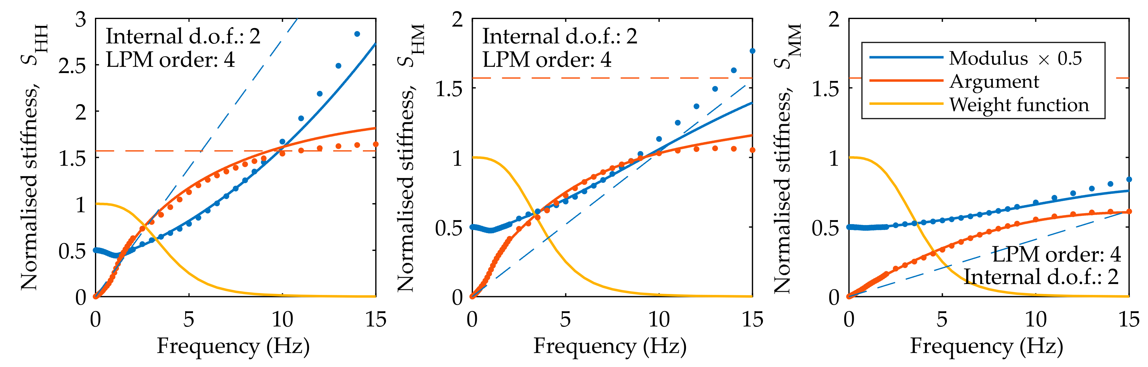
3.4. Calibration and Test of Lumped-Parameter Model

For the components, $D_{\mathrm{HH}}\left(\omega \right)$, $D_{\mathrm{MM}}\left(\omega \right)$, and $D_{\mathrm{HM}}\left(\omega \right)$, fourth-order lumped-parameter models are found to provide accurate approximations. Figure 3 shows the fitted LPM solution as well as the target solution and the weight function, $w\left(a_0\right)=w\left(\omega R_{\mathrm{p}}/c_{\mathrm{S}}\right)$, in the frequency range 0–15 Hz. The complex-valued normalized stiffnesses are presented in terms of their modulus (note the factor 0.5) and argument.

Figure 3 shows that the dynamic stiffness is nearly the same as the static stiffness for frequencies up to about 0.5 Hz. A local dip occurs in the modulus around 1 Hz. Thus, the considered normalized stiffness components decrease by about 10% from 1 in the static limit to values of around 0.9 at 1 Hz. Referring to the previous comparison of the beam and shell models of the pile, it is anticipated that this will induce a 1% reduction in the second eigenfrequency of the OWT system.

In the frequency range around the local dip in the moduli of the stiffness components, the arguments (or phase angles) increase rapidly, and a further increase occurs until the arguments reach more or less constant values of 0.5–1.5 at higher frequencies. At the same time, the modulus increases more than linearly for frequencies above 1 Hz. This is caused by geometrical damping related to wave radiation away from the monopile and into the soil, as the frequency becomes higher than the cut-on frequency for wave propagation in the top layer. This dissipation can be expected to propagate into damping of the OWT.

To match the target solution calculated by the method presented in Section 3.1, a sixth-order LPM must be used for the vertical component (not illustrated in the figure). Discrete-element systems with one internal degree of freedom per every second order of the lumped-parameter model are used in all cases. Since the coupling terms $D_{\mathrm{HM}}\left(\omega \right)$ and $D_{\mathrm{MH}}\left(\omega \right)$ need independent treatment, a total of $2+2+\left(2\times 2\right)+3$ internal d.o.f. are considered in the LPM for the pile-subsoil system.

4. Influence of Model Simplifications

The response of the wind-turbine structure is calculated for the three load cases described in Section 2.3. For comparison with the model employing the LPM for the pile–subsoil system, analyses have been carried out using the static pile-cap stiffness. The results are presented in Figure 4 and Figure 5 in terms of time series and spectra for the external moments, $M$, and the bending moments, $M_y$. The considered wave peaks occur around 5400 s into the 3-h simulation.

To eliminate errors associated with false initial conditions, two adjustments are made. First, the structure is subjected to a 12-min wave train prior to application of the simulated wave. Second, tapering of the wave forces is introduced, employing a cosine taper function with a duration of 1.0 min to reach full magnitude of the wave forces. Before calculating frequency spectra by inverse Fourier transformation, the same taper function is applied to the time series, starting 2.0 min before the simulated wave with 1.0 min of tapering, and ending 4.0 min after the considered wave with 1.0 min of tapering. Thus, the full magnitude is present 1.0 min before the wave in question, and 3.0 min of trailing waves are considered. This duration is chosen in order to capture the nature and frequency content of the response brought about by the various load cases and the two different models of the foundation.

As a first observation, Case 2 (the single higher-order wave) provides external moments, $M$, and bending moments, $M_y$, that are significantly (about 75%) higher than Case 1 (the linear irregular waves). Case 3 (the slamming wave) only leads to an additional 5–10% increase. This may be caused by the choice made in relation to Equation (2), namely, that the fluid particle velocity in front of the pile is considered for the calculation of the slamming load. Hence, the slamming load provides its main contribution almost in phase with the drag term from the Morison equation and it is recalled that the wave loads in the present case are already drag-dominated. In a case with inertia-dominated wave loads, or with a different assumption being made regarding the fluid particle velocities related to slamming, the relative importance of the higher-order wave theory becomes slightly smaller and the importance of slamming increases significantly.

Regarding the maximum bending moments at mudline, marginal differences (only about 1%) occur between models with and without the LPM in the present example. However, this may change if one or more higher-order waves, possibly slamming waves, hit the structure before the vibration caused by the first higher-order (slamming) wave has diminished.

In Case 1, for the first eigenmode, resonance peaks in the Fourier amplitude spectra for all cases are approximately 3% higher in the model with static pile-cap stiffness compared to the model with the LPM, indicating a slight overestimation of vibration levels with the simpler foundation model. In contrast, Case 3 produces a response that is nearly twice the magnitude of the response in Case 1, indicating that the wave load model has greater effect than the foundation model.

Evidently, Cases 2 and 3 produce much more significant oscillations in the second and third eigenmodes compared with Case 1. In the second eigenmode, Case 3 provides a resonance peak about 10% higher than that of Case 2 and nearly a full order of magnitude higher than that of Case 1. In the third eigenmode, the wave slamming has negative impact on the moments. Hence, the external moment as well as the bending moment in Case 3 are less than half of those observed in Case 2., though still about twice the values occurring in Case 1. For Modes 2 and 3, the influence of simplifying the foundation model also becomes more pronounced. The model with static pile-cap stiffness overestimates the response related to Mode 2 by a factor of two and, for Mode 3, the response is three times higher with the simplified model than with the model including the LPM. Hence, model uncertainty and the effect of using an inadequate foundation model is much more pronounced in Modes 2 and 3 compared with Mode 1. This can be explained by the fact that the response of the pile and subsoil is nearly quasi-static at frequencies well below 1 Hz. On the other hand, as discussed in the previous section, radiation of energy into the far field within the soil is introduced at frequencies higher than about 0.5 Hz. Compared to the material dissipation (the only other source of dissipation considered in the present analysis), the geometrical damping is significant.

5. Conclusions

This study focused on uncertainties related to the use of simplified soil–structure interaction models to represent offshore wind turbines supported by monopile foundations. In particular, comparisons were made regarding the system response obtained by using static pile-cap stiffness and lumped-parameter models. Different wave-load cases were compared, with wind loads omitted. These cases included linear irregular waves (with a significant wave height of 10 m) as well as a highly nonlinear wave merged into an irregular wave train. With the nonlinear wave, inclusion and exclusion of slamming loads were also studied. Time series and Fourier amplitude spectra for external bending moments and for mudline bending moments were studied for three different load cases, focusing on the extreme loads and on resonance peaks and frequency content in the response.

In general, it is found that the fundamental frequency response of the system—which, at 0.2 Hz, is significantly below 1 Hz—is well-represented by the static pile-cap stiffness model, since the soil and subsoil behave almost quasi-statically then. In contrast, resonance contributions related to the second and third modes of the system (around 1 Hz and 2 Hz, respectively) are overestimated by the static pile-cap model. The effects are more pronounced when a nonlinear wave theory is employed. For a drag-dominated wave load considered in the present analyses, wave slamming provides increases in the load magnitudes related to eigenmodes 1 and 2 of the considered system. On the other hand, slamming causes a decrease of the load associated with eigenmode 3.

This study highlights the role that uncertainty in models for soil–structure interaction can play in dealing with bottom-supported offshore wind turbines with monopile foundations. Future research may focus on further development of dynamic load and structure–water–soil interaction models that can aid the design of new offshore wind turbines without compromising computational cost.

References

1. Damgaard, M.; Zania, V.; Andersen, L.V.; Ibsen, L.B. Effects of soil-structure interaction on real time dynamic response of offshore wind turbines on monopiles. Eng. Struct. 2014, 75, 388–401. [Google Scholar] [CrossRef]
2. Byrne, B.; Mcadam, R.; Burd, H.; Houlsby, G.; Martin, C.; Beuckelaers, W.; Zdravkovic, L.; Taborda, D.M.G.; Potts, D.; Jardine, R.; et al. PISA: New Design Methods for Offshore Wind Turbine Monopiles. In Proceedings of the Royal Geographical Society 8th International Conference (OSIG 2017), London, UK, 12–14 September 2017; Society for Underwater Technology: London, UK, 2017; pp. 142–161. [Google Scholar] [Green Version]
3. Thieken, K.; Achmus, M.; Lemke, K. A new static p-y approach for piles with arbitrary dimensions in sand. Geotechnik 2015, 38, 267–288. [Google Scholar] [CrossRef]
4. Vahdatirad, M.J.; Bayat, M.; Andersen, L.V.; Ibsen, L.B. Probabilistic finite element stiffness of a laterally loaded monopile based on an improved asymptotic sampling method. J. Civ. Eng. Manag. 2015, 21, 503–513. [Google Scholar] [CrossRef]
5. Andersen, L.V.; Vahdatirad, M.J.; Sichani, M.T.; Sørensen, J.D. Natural frequencies of wind turbines on monopile foundations in clayey soils-A probabilistic approach. Comput. Geotech. 2012, 43, 1–11. [Google Scholar] [CrossRef]
6. Versteijlen, W.G.; Metrikine, A.V.; van Dalen, K.N. A method for identification of an effective Winkler foundation for large-diameter offshore wind turbine support structures based on in-situ measured small-strain soil response and 3D modelling. Eng. Struct. 2016, 124, 221–236. [Google Scholar] [CrossRef]
7. Amar Bouzid, D.; Bhattacharya, S.; Otsmane, L. Assessment of natural frequency of installed offshore wind turbines using nonlinear finite element model considering soil-monopile interaction. J. Rock Mech. Geotech. Eng. 2018, 10, 333–346. [Google Scholar] [CrossRef]
8. Achmus, M.; Abdel-Rahman, K.; Kuo, Y. Numerical modelling of large diameter steel piles under monotonic and cyclic horizontal loading. In Numerical Models in Geomechanics; Taylor & Francis: London, UK, 2007. [Google Scholar] [CrossRef] [Green Version]
9. Wolf, J.; Meek, J.; Sung, C. Cone models for a pile foundation. In Piles under Dynamic Loads; Geotechnical Special Publications; ASCE: New York, NY, USA, 1992; Volume 34, pp. 94–113. [Google Scholar]
10. Wolf, J.P. Consistent lumped-parameter models for unbounded soil: Frequency-independent stiffness, damping and mass matrices. Earthq. Eng. Struct. Dyn. 1991, 20, 33–41. [Google Scholar] [CrossRef]
11. Wolf, J.P. Consistent lumped-parameter models for unbounded soil: Physical representation. Earthq. Eng. Struct. Dyn. 1991, 20, 11–32. [Google Scholar] [CrossRef]
12. Cook, R.D.; Malkus, D.S.; Plesha, M.E.; Witt, R.J. Concepts and Applications of Finite Element Analysis; John Wiley & Sons, Inc.: New York, NY, USA, 2002. [Google Scholar]
13. Morison, J.R.; Johnson, J.W.; Schaaf, S.A. The Force Exerted by Surface Waves on Piles. J. Pet. Technol. 1950, 2, 149–154. [Google Scholar] [CrossRef]
14. Det Norske Veritas. DNV-RP-J101: Design of Offshore Wind Turbine Structures; Det Norske Veritas: Hovik, Norway, 2014. [Google Scholar]
15. Wheeler, J.D. Method for Calculating Forces Produced by Irregular Waves. J. Pet. Technol. 1970, 22, 359–367. [Google Scholar] [CrossRef]
16. Rienecker, M.M.; Fenton, J.D. A Fourier approximation method for steady water waves. J. Fluid Mech. 1981, 104, 119. [Google Scholar] [CrossRef]
17. Rendon, E.A.; Manuel, L. Long-term loads for a monopile-supported offshore wind turbine. Wind Energy 2014, 17, 209–223. [Google Scholar] [CrossRef]
18. Senanayake, A.; Manuel, L.; Gilbert, R.B. Estimating natural frequencies of monopile supported offshore wind turbines using alternative P-Y models. In Proceedings of the Annual Offshore Technology Conference, Houston, TX, USA, 1–4 May 2017; Volume 6. [Google Scholar]
19. Andersen, L.; Clausen, J. Impedance of surface footings on layered ground. Comput. Struct. 2008, 86, 72–87. [Google Scholar] [CrossRef]
20. Liingaard, M.; Andersen, L.; Ibsen, L.B. Impedance of flexible suction caissons. Earthq. Eng. Struct. Dyn. 2007, 36, 2249–2271. [Google Scholar] [CrossRef] [Green Version]
21. Andersen, L.V. Influence of dynamic soil-structure interaction on building response to ground vibration. In Numerical Methods in Geotechnical Engineering: Proceedings of the 8th European Conference on Numerical Methods in Geotechnical Engineering NUMGE, Delft, The Netherlands, 18–20 June 2014; CRC Press: Boca Raton, FL, USA, 2014; Volume 2, pp. 1087–1092. [Google Scholar]
22. Andersen, L. Assessment of lumped-parameter models for rigid footings. Comput. Struct. 2010, 88, 1333–1347. [Google Scholar] [CrossRef]
23. Damgaard, M.; Andersen, L.V.; Ibsen, L.B. Computationally efficient modelling of dynamic soil-structure interaction of offshore wind turbines on gravity footings. Renew. Energy 2014, 68, 289–303. [Google Scholar] [CrossRef]
Figure 1. Model of soil–pile interaction using Green’s function.
Jmse 06 00087 g001
Figure 2. Undamped tower eigenmodes and corresponding eigenfrequencies (blue/yellow shades indicate compression/tension).
Jmse 06 00087 g002
Figure 3. Fitting of lumped-parameter models for the coupled horizontal translation and rocking rotation of the pile cap (dots indicate target solution; dashed lines indicate high-frequency limit).
Jmse 06 00087 g003
Figure 4. Time series and Fourier amplitude spectra of external moments and mudline moments for the lumped-parameter model (LPM) of the pile–subsoil system, considering all load cases.
Jmse 06 00087 g004
Figure 5. Time series and Fourier amplitude spectra of external moments and mudline moments for the model with static pile-cap stiffness, considering all load cases.
Jmse 06 00087 g005