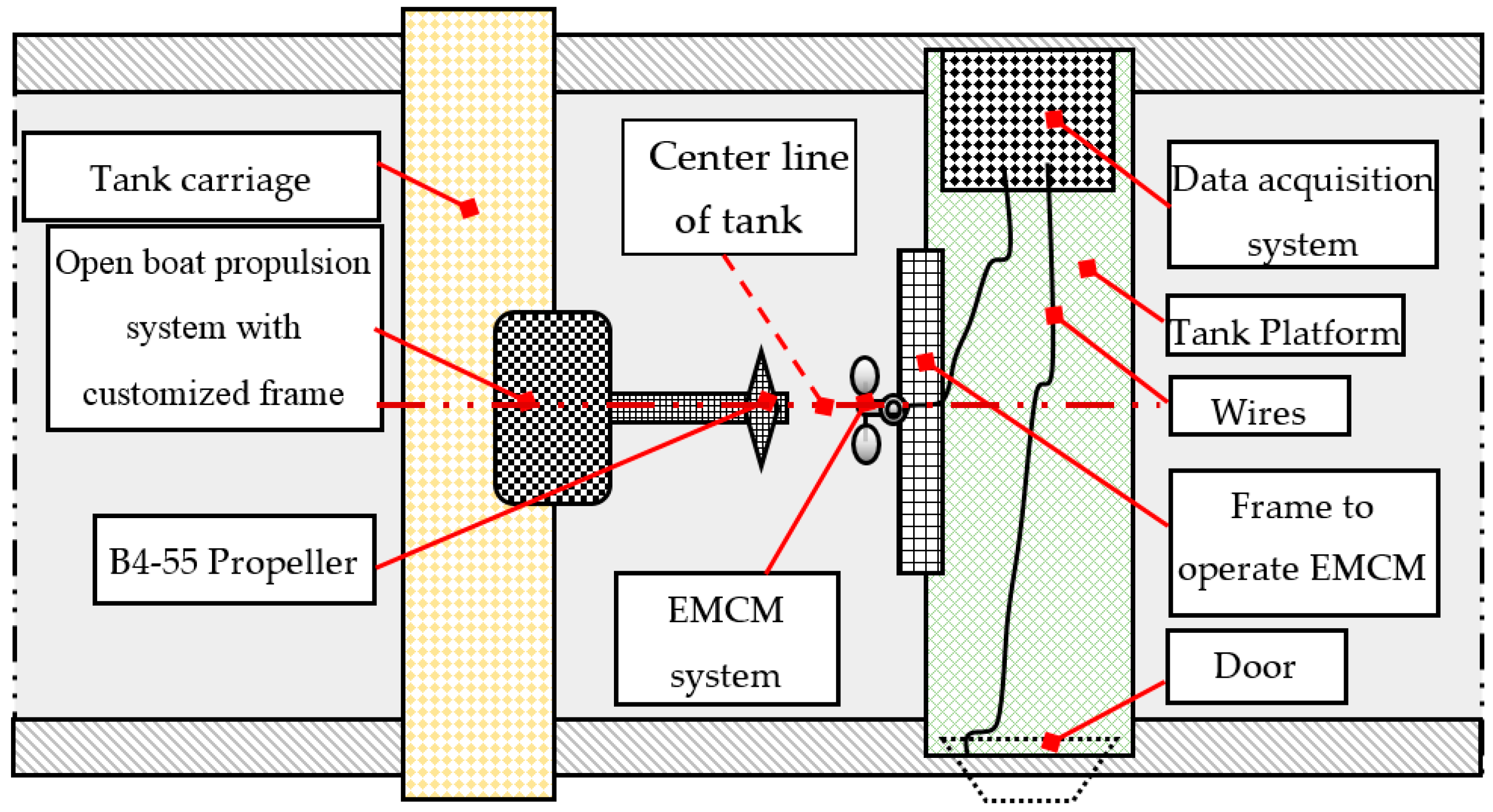
Figure 1.
Schematic of experimental set-up.
Figure 1.
Schematic of experimental set-up.
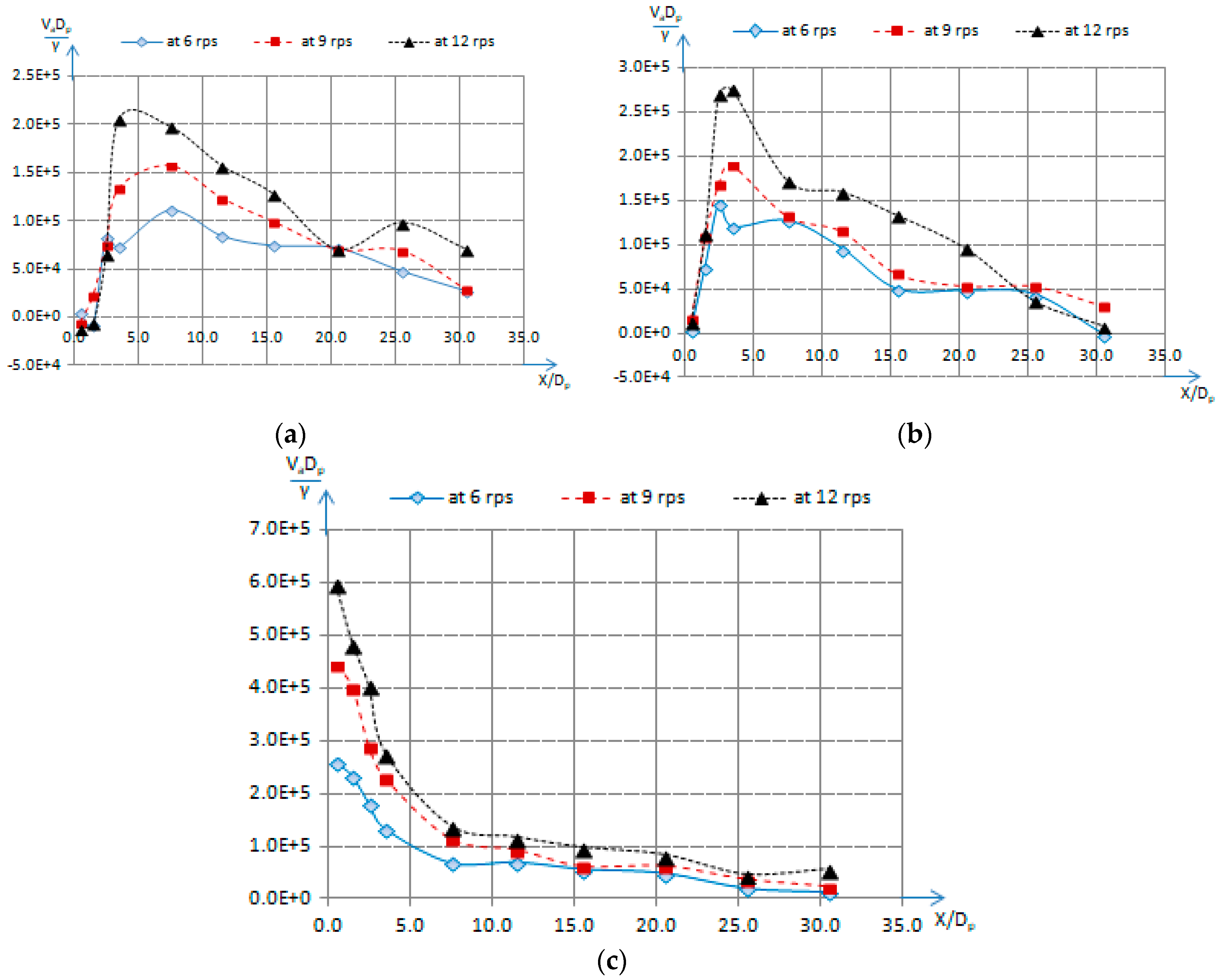
Figure 2.
(a) Mean axial flow velocity along x/Dp at y/Dp = 0 and d = 0.25Dp for different ‘n’; (b) Mean axial flow velocity along x/Dp at y/Dp = 0 and d = 0.55Dp for different ‘n’; (c) Mean axial flow velocity along x/Dp at y/Dp = 0 and d = 1.05Dp for different ‘n’.
Figure 2.
(a) Mean axial flow velocity along x/Dp at y/Dp = 0 and d = 0.25Dp for different ‘n’; (b) Mean axial flow velocity along x/Dp at y/Dp = 0 and d = 0.55Dp for different ‘n’; (c) Mean axial flow velocity along x/Dp at y/Dp = 0 and d = 1.05Dp for different ‘n’.
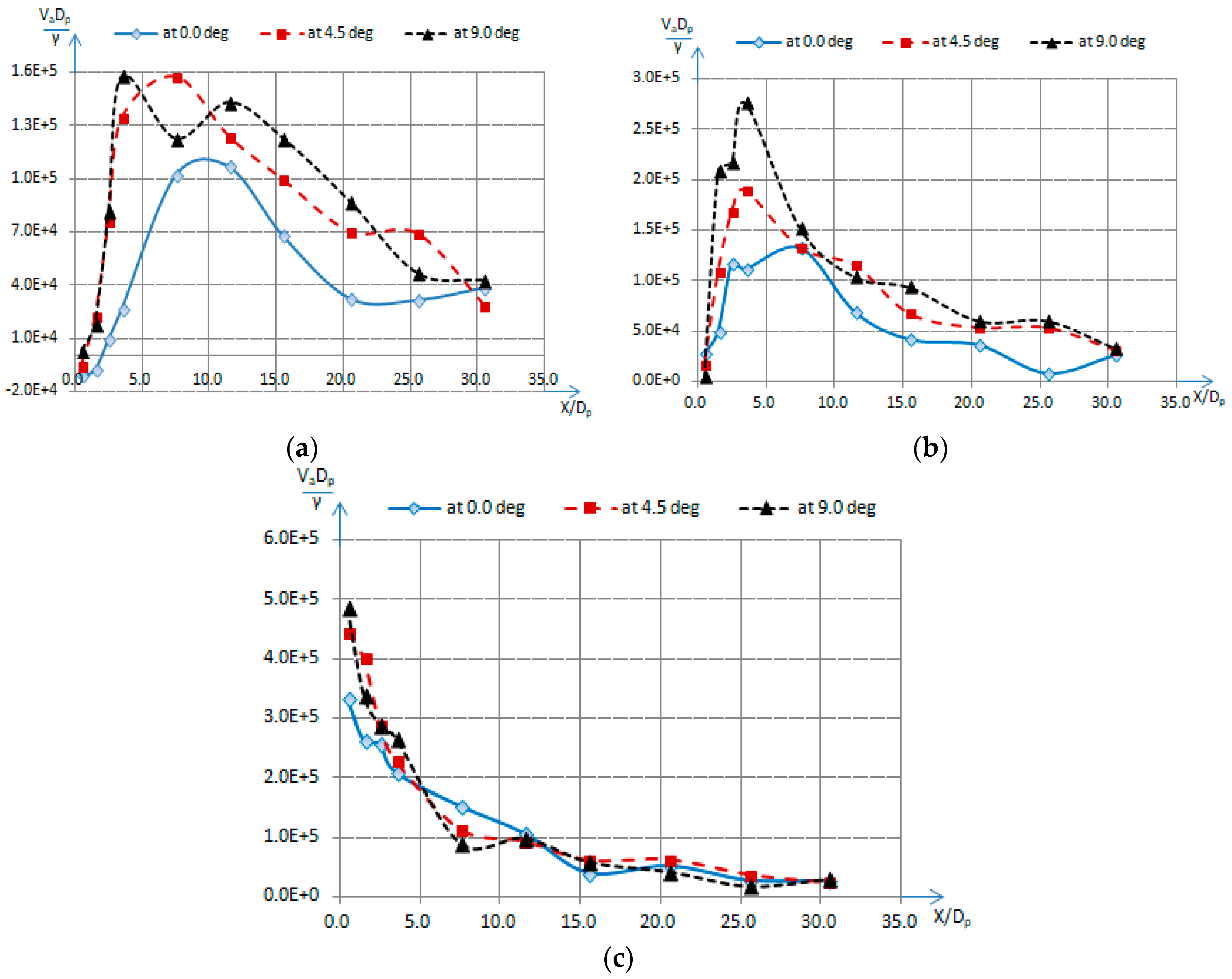
Figure 3.
(a) Mean axial flow velocity along x/Dp at y/Dp = 0 and d = 0.25Dp for different ‘θ’; (b) mean axial flow velocity along x/Dp at y/Dp = 0 and d = 0.55Dp for different ‘θ’; (c) mean axial flow velocity along x/Dp at y/Dp = 0 and d = 1.05Dp for different ‘θ’.
Figure 3.
(a) Mean axial flow velocity along x/Dp at y/Dp = 0 and d = 0.25Dp for different ‘θ’; (b) mean axial flow velocity along x/Dp at y/Dp = 0 and d = 0.55Dp for different ‘θ’; (c) mean axial flow velocity along x/Dp at y/Dp = 0 and d = 1.05Dp for different ‘θ’.
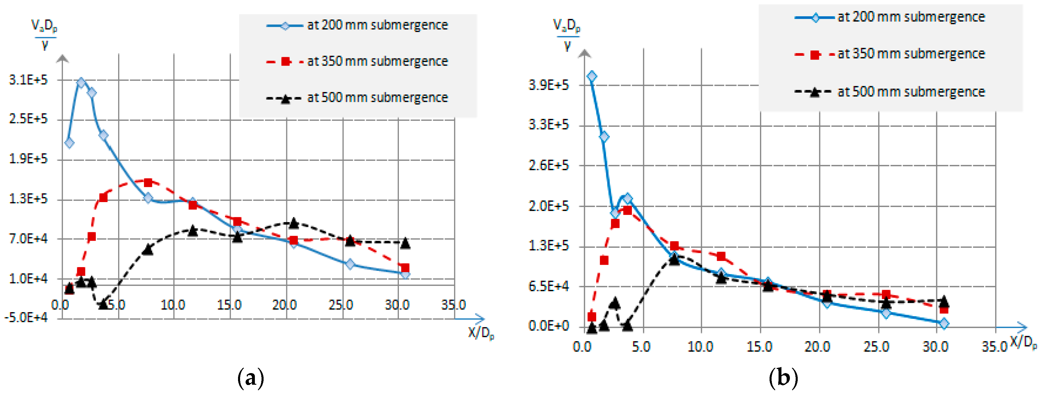
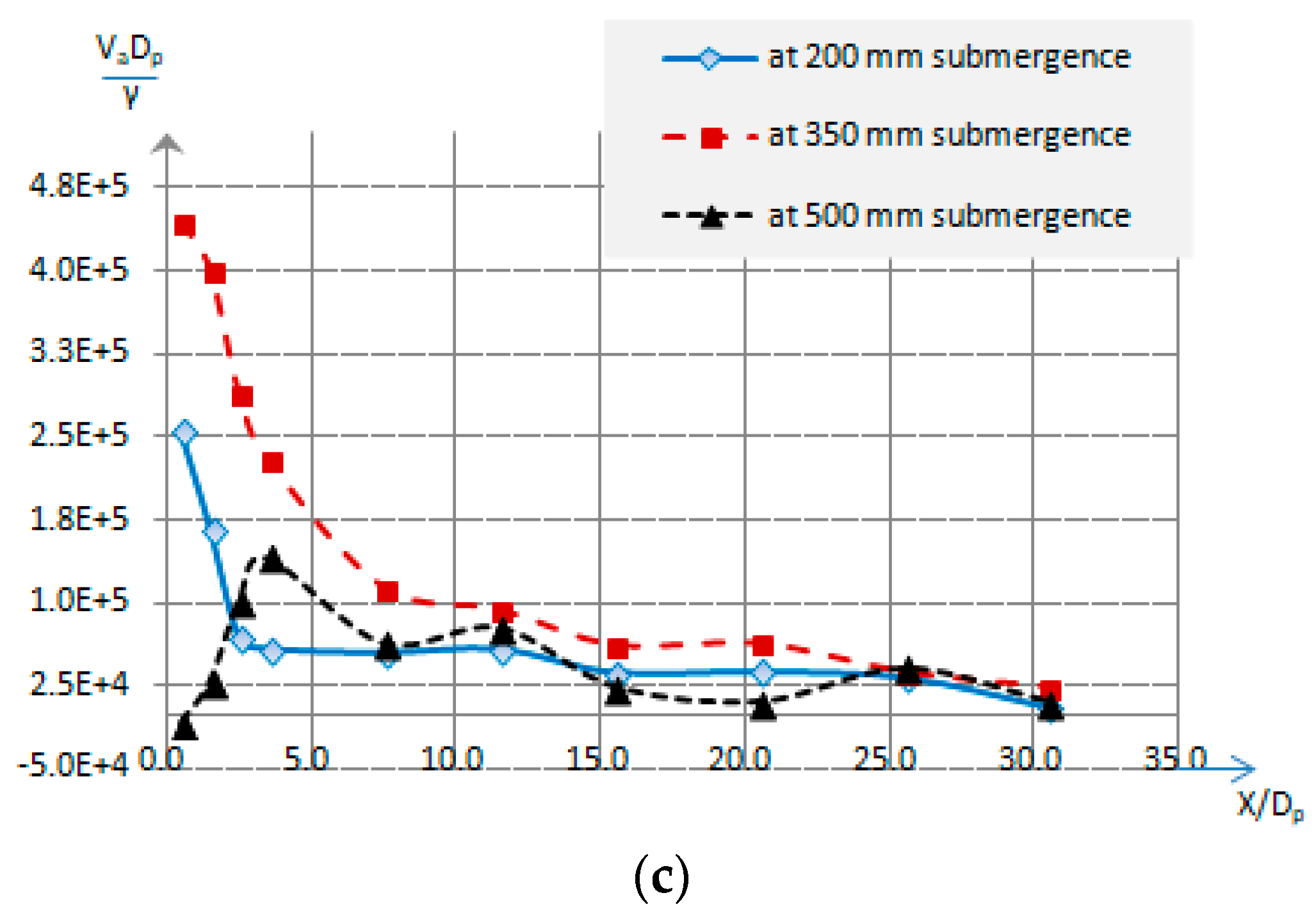
Figure 4.
(a) Mean axial flow velocity along x/Dp at y/Dp = 0 and at d = 0.25Dp for different ‘H’; (b) mean axial flow velocity along x/Dp at y/Dp = 0 and at d = 0.55Dp for different ‘H’; (c) mean axial flow velocity along x/Dp at y/Dp = 0 and at d = 1.05Dp for different ‘H’.
Figure 4.
(a) Mean axial flow velocity along x/Dp at y/Dp = 0 and at d = 0.25Dp for different ‘H’; (b) mean axial flow velocity along x/Dp at y/Dp = 0 and at d = 0.55Dp for different ‘H’; (c) mean axial flow velocity along x/Dp at y/Dp = 0 and at d = 1.05Dp for different ‘H’.
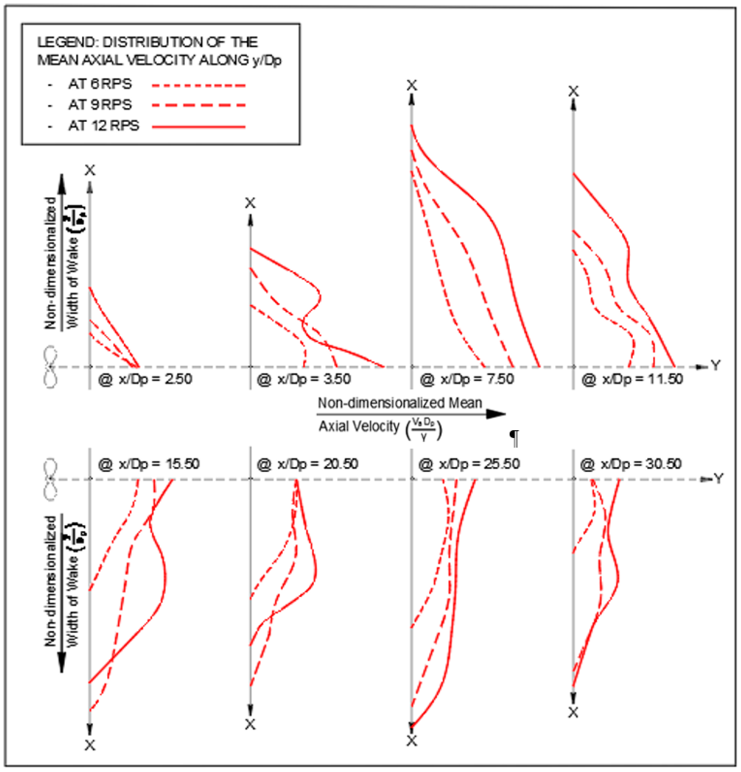
Figure 5.
The approximate patterns of the distribution of the non-dimensionalized mean axial velocities along y/Dp with the change of ‘n’.
Figure 5.
The approximate patterns of the distribution of the non-dimensionalized mean axial velocities along y/Dp with the change of ‘n’.
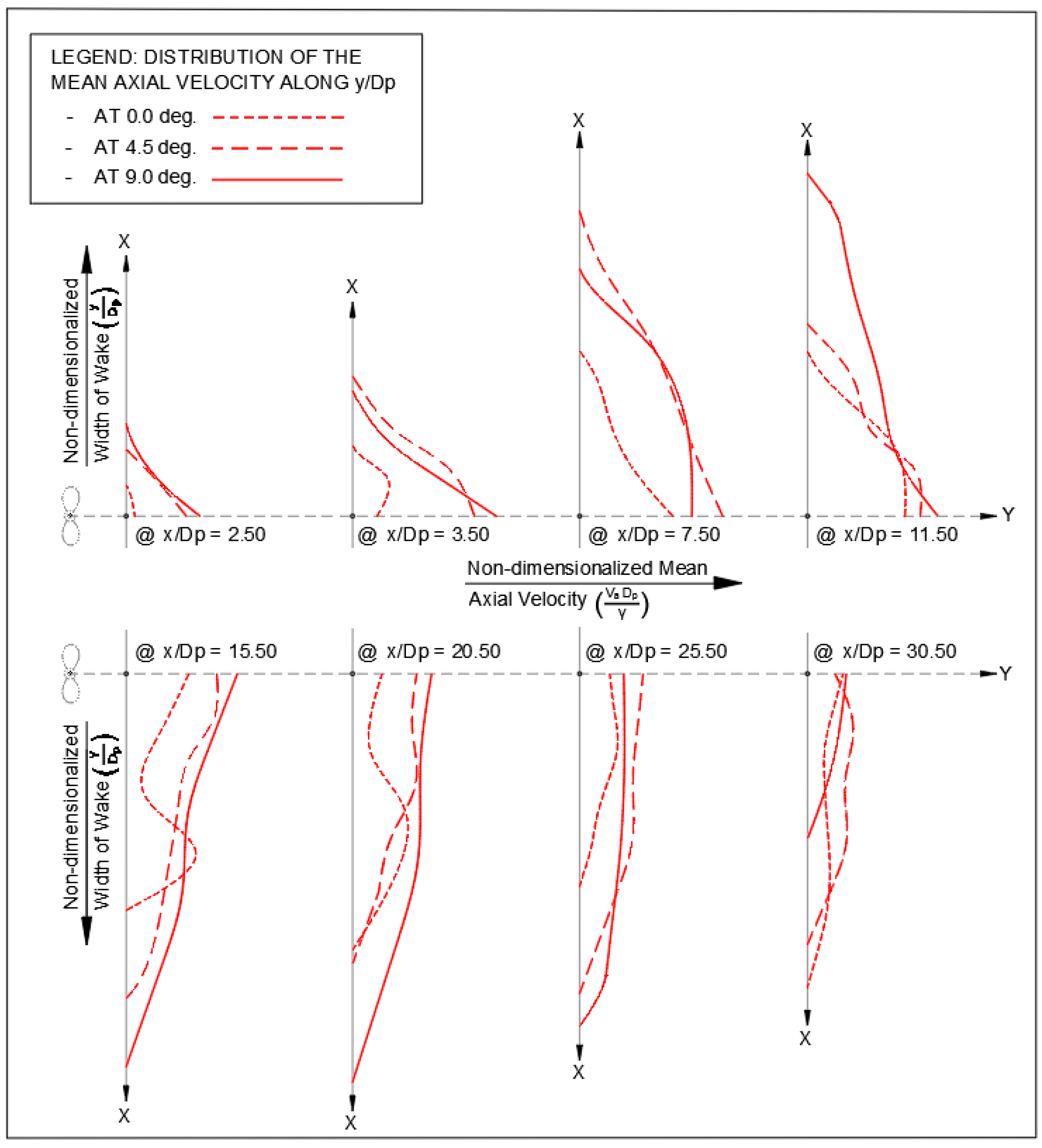
Figure 6.
The approximate patterns of the distribution of the non-dimensionalized mean axial velocities along y/Dp with the change of ‘θ’.
Figure 6.
The approximate patterns of the distribution of the non-dimensionalized mean axial velocities along y/Dp with the change of ‘θ’.
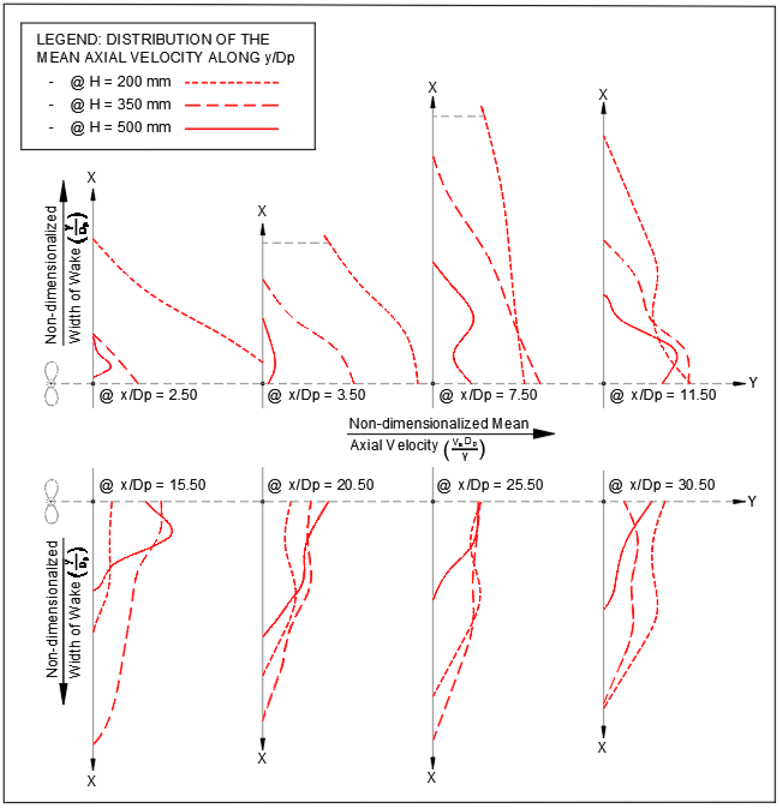
Figure 7.
The approximate patterns of the distribution of the non-dimensionalized mean axial velocities along y/Dp with the change of ‘H’.
Figure 7.
The approximate patterns of the distribution of the non-dimensionalized mean axial velocities along y/Dp with the change of ‘H’.
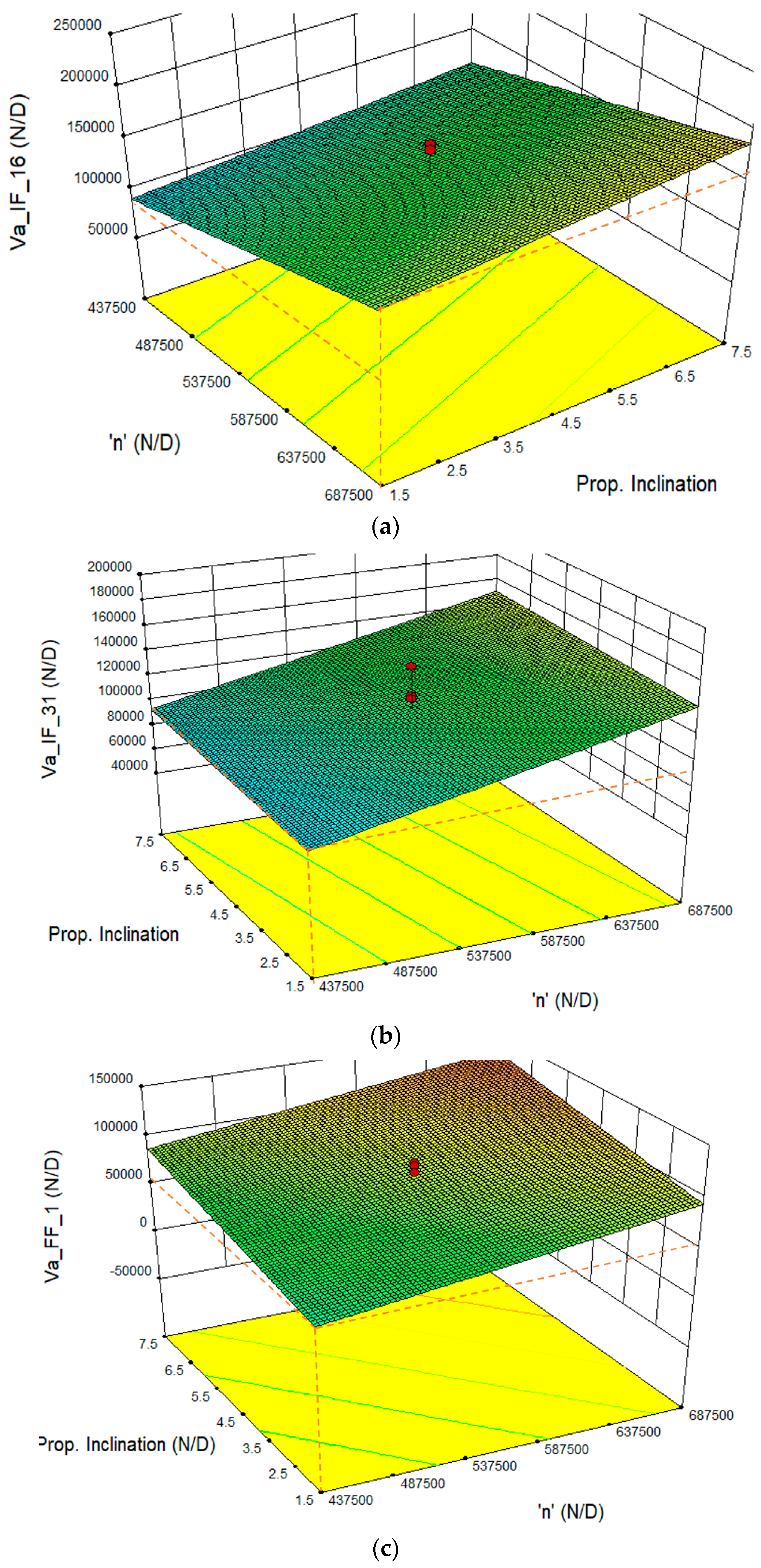
Figure 8.
(a) 3D surface plot showing the interaction effect of ‘n’ and ‘θ’ on the mean axial flow velocity at the point location of (x/Dp, y/Dp, d/Dp) = (7.5, 0.0, 0.25); (b) 3D surface plot showing the interaction effect of ‘n’ and ‘θ’ on the mean axial flow velocity at the point location of (x/Dp, y/Dp, d/Dp) = (11.5, 0.0, 0.25); (c) 3D surface plot showing the interaction effect of ‘n’ and ‘θ’ on the mean axial flow velocity at the point location of (x/Dp, y/Dp, d/Dp) = (15.5, 0.0, 0.25).
Table 1.
Factors used at different levels of the experiment.
Table 1.
Factors used at different levels of the experiment.
| Factors | Low Axial (−1.5) | Low (−1) | Center (0) | High (+1) | High Axial (+1.5) |
|---|
| Shaft rotational speed (rps) | 6.0 | 7.0 | 9.0 | 11.0 | 12.0 |
| Propeller inclination (deg.) | 0.0 | 1.5 | 4.5 | 7.5 | 9.0 |
| Submergence of propeller (mm) | 200 | 250 | 350 | 450 | 500 |
Table 2.
Properties of the model propeller.
Table 2.
Properties of the model propeller.
| Diameter, Dp | 250 mm | Bollard thrust coeff., Ct | 0.306 |
| Hub diameter, Dh | 42 mm | Bollard torque coeff., Cq | 0.041 |
| Blade Area Ratio, β | 55 | Number of blades, N | 4 |
Table 3.
Combinations of factors under each case to assess the individual effect of factors.
Table 3.
Combinations of factors under each case to assess the individual effect of factors.
| Case #1: Influence of Propeller Rotational Speed ‘n’ on the Mean Axial Velocity of Flow |
| Selected Runs | ‘n’ in rps | ‘θ’ in degree | ‘H’ in mm |
| Run #1 | 6 | 4.5 | 350 |
| * Center Point Run | 9 | 4.5 | 350 |
| Run #16 | 12 | 4.5 | 350 |
| Case #2: Influence of Propeller Inclination Angle ‘θ’ on the Mean Axial Velocity of Flow |
| Selected Runs | ‘n’ in rps | ‘θ’ in degree | ‘H’ in mm |
| Run #5 | 9 | 0.0 | 350 |
| * Center Point Run | 9 | 4.5 | 350 |
| Run #2 | 9 | 9.0 | 350 |
| Case #3: Influence of Propeller Depth of Submergence ‘H’ on the Mean Axial Velocity of Flow |
| Selected Runs | ‘n’ in rps | ‘θ’ in degree | ‘H’ in mm |
| Run #14 | 9 | 4.5 | 200 |
| * Center Point Run | 9 | 4.5 | 350 |
| Run #13 | 9 | 4.5 | 500 |
Table 4.
Regression equations for predicting K, a, b, c, a1, b1, c1, a2, b2 and c2 for Near Field.
Table 4.
Regression equations for predicting K, a, b, c, a1, b1, c1, a2, b2 and c2 for Near Field.
| Coeff. of (A) ‘K’–‘c2’ | Prediction Equations of the Unknown Coefficients (K~c2) for Near Field zone, Obtained through Stepwise Regression Analysis Incorporating up to Cubic Terms |
| K | K = 479,548 − {258,367 × (y/Dp)} − {1,075,757 × (d/Dp) × (d/Dp) × (d/Dp)} + {1,399,716 × (d/Dp) × (d/Dp) × (y/Dp)} − {561,931 × (d/Dp) × (y/Dp) × (y/Dp)} |
| a | a = 0.369 − {0.052 × (x/Dp)} + {0.0336 × (y/Dp)} – {0.030 × (d/Dp)} |
| b | b = 34,935 + {19,327 × (x/Dp)} − {121,413 × (d/Dp)} − {28,062 × (y/Dp)} − {5435 × (x/Dp) × (x/Dp)} + {85,102 × (d/Dp) × (y/Dp)} |
| c | c = −520,828 + {343,649 × (y/Dp) × (y/Dp)} + {1,656,413 × (d/Dp) × (d/Dp) × (d/Dp)} − {1,321,759 × (d/Dp) × (d/Dp) × (y/Dp)} |
| a1 | Ignored, as this coefficient is too small (average = 5.70 × 10⁻³) to affect the field |
| b1 | b1 = −0.069 − {0.344 × (x/Dp)} − {0.470 × (d/Dp)} + {0.574 × (y/Dp)} + {0.0515 × (x/Dp) × (x/Dp)} − {0.245 × (y/Dp) × (y/Dp)} + {0.379 × (x/Dp) × (d/Dp)} + {0.0367 × (x/Dp) × (y/Dp)} + {0.191 × (d/Dp) × (y/Dp)} − {0.190 × (x/Dp) × (d/Dp) × (y/Dp)} |
| c1 | c1 = −10,949 + {3232 × (x/Dp)} + {44,920 × (d/Dp) × (y/Dp)} + {57,454 × (d/Dp) × (d/Dp) × (d/Dp)} − {82,479 × (d/Dp) × (d/Dp) × (y/Dp)} |
| a2 | Ignored, as this coefficient is too small (average = 9.69 × 10⁻⁹) to affect the field |
| b2 | b2 = 0.369 − {0.052 × (x/Dp)} + {0.0336 × (y/Dp)} − {0.03033 × (d/Dp)} |
| c2 | c2 = 223,033 − {790,287 × (d/Dp) × (y/Dp)} − {705,383 × (d/Dp) × (d/Dp) × (d/Dp)} + {1,155,228 × (d/Dp) × (d/Dp) × (y/Dp)} |
Table 5.
Regression equations for predicting K, a, b, c, a1, b1, c1, a2, b2 and c2 for the Intermediate Field.
Table 5.
Regression equations for predicting K, a, b, c, a1, b1, c1, a2, b2 and c2 for the Intermediate Field.
| Coeff. of (A) ‘K’–‘c2’ | Prediction Equations of the Unknown Coefficients (K~c2) for the Intermediate Field, Obtained through Stepwise Regression Analysis Incorporating up to Cubic Terms |
|---|
| K | K = 53,956 − {456,792 × (y/Dp)} + {278,313 × (y/Dp) × (y/Dp)} − {40,801 × (y/Dp) × (y/Dp) × (y/Dp)} |
| a | a = 0.3135 − {0.0055 × (x/Dp)} − {0.288 × (y/Dp)} − {0.0243 × (d/Dp)} |
| b | b = −7788 + {4985 × (y/Dp)} |
| c | c = 143,033 + {229,377 × (y/Dp)} − {194,465 × (y/Dp) × (y/Dp)} + {30,873 × (y/Dp) × (y/Dp) × (y/Dp)} |
| a1 | a1 = 0.011 − {0.007 × (y/Dp)} |
| b1 | b1 = −0.154 + {0.356 × (d/Dp)} − {0.092 × (y/Dp)} + {0.0335 × (y/Dp) × (y/Dp)} − {0.084 × (d/Dp) × (y/Dp)} |
| c1 | c1 = 22,893 − {1396 × (x/Dp)} − {7321 × (y/Dp)} + {481 × (x/Dp) × (y/Dp)} |
| a2 | Ignored, as this coefficient is too small (average = 9.61 × 10⁻⁸) to affect the field |
| b2 | b2 = −1173 + {719 × (d/Dp)} − {1032−(y/Dp)} + {763 × (y/Dp) × (y/Dp)} − {116.2 × (y/Dp) × (y/Dp) × (y/Dp)} |
| c2 | c2 = −99,090 + {34,803 × (y/Dp)} |
Table 6.
Regression equations for predicting K, a, b, c, a1, b1, c1, a2, b2 and c2 for the Far Field.
Table 6.
Regression equations for predicting K, a, b, c, a1, b1, c1, a2, b2 and c2 for the Far Field.
| Coeff. of (A) ‘K’–‘c2’ | Prediction Equations of the Unknown Coefficients (K~c2) for the Far Field, Obtained through Stepwise Regression Analysis Incorporating up to Cubic Terms |
|---|
| K | K = 134,120 − {6844 × (x/Dp)} |
| a | a = −0.267 + {0.349 × (d/Dp)} + {0.1685 × (y/Dp)} − {0.206 × (d/Dp) × (y/Dp)} |
| b | b = 5491 − {467 × (x/Dp) × (d/Dp)} + {10,933 × (d/Dp) × (d/Dp) × (d/Dp)} |
| c | c = −852,767 + {54,310 × (x/Dp)} + {488,902 × (d/Dp)} + {132,689 × (y/Dp)} − {902 × (x/Dp) × (x/Dp)} − {20,372 × (y/Dp) × (y/Dp)} − {10,354 × (x/Dp) × (d/Dp)} − {194,760 × (d/Dp) × (y/Dp)} + {25,978 × (d/Dp) × (y/Dp) × (y/Dp)} |
| a1 | Ignored, as this coefficient is too small (average = 1.66 × 10⁻³) to affect the field |
| b1 | b1 = 0.0546 − {0.0334 × (y/Dp)} + {0.0388 × (d/Dp) × (d/Dp) × (y/Dp)} |
| c1 | c1 = 3713 − {5329 × (d/Dp) × (d/Dp) × (d/Dp)} |
| a2 | Ignored, as this coefficient is too small (average = −4.76 × 10⁻⁹) to affect the field |
| b2 | b2 = −647 + {360 × (d/Dp)} |
| c2 | c2 = −657,734 + {94,409 × (x/Dp)} + {78,090 × (y/Dp)} − {4593 × (x/Dp) × (x/Dp)} − {11,756 × (y/Dp) × (y/Dp)} − {3454 × (x/Dp) × (y/Dp)} + {71.8 × (x/Dp) × (x/Dp) × (x/Dp)} + {570 × (x/Dp) × (y/Dp) × (y/Dp)} |


