1. Introduction
There has been increasing concern regarding the environmental effect of seabed vibration caused by impacts generated during offshore construction, such as the installation of marine renewable energy devices and offshore oil and gas platforms. These have been considered by Thomsen et al. [
1] (MaRVEN report) and Popper et al. [
2]. An important source of such seabed impact is marine pile driving. Whilst there have been a number of studies of the sound radiated into the water column by Reinhall et al. [
3], Zampolli et al. [
4] and Lippert et al. [
5], there have been relatively few on seabed vibration such as Reiman et al. [
6]. The work described here began with an experiment which measured seismic waves propagating across the seabed, and then used transient finite element models which could link the sediment motion to the acoustic pressure and motions of the water above.
Within the MarVEN [
1] report the effects of “Ground roll waves emitted during pile driving” are cited as a key knowledge gap. Earlier concerns led to studies of both piling [
7] and dredging [
8] in 2010. A seismometer sledge was designed to be deployed in shallow (<40 m) water. It used a triaxial set of geophones on a stainless steel base, which could be aligned by being towed a short distance across the seabed. The seismometer was deployed near a test piling operation in a dock at Kinderdijk, The Netherlands, alongside a hydrophone array [
7]. The same sledge was used offshore (English Channel), deployed from a ship anchored near a dredging operation [
8].
At Kinderdijk, slow infrasonic waves were seen to follow the arrival of water borne sound. Whilst generated by the same regular blows to the test pile, these had the tonal characteristics of a seismic wavelet. The contrast between these wave pulses has been studied using finite element analysis (FEA). Rather than trying to mimic the reverberant field conditions and the detailed pile structure, the later FEA models were made axisymmetric, with an idealized vertical impact applied to a graded seabed structure, without any nearby reflectors. The observed timing and frequency characteristics were replicated in large measure by this modeling, based on Hamilton’s data [
9] for seabed material properties. Most of the models used a transient analysis, but as expected, this layered structure, when forced by a continuous sinusoid, showed a variable wave speed with frequency, a “dispersive” response. However, most of the wavelet energy envelopes, as excited by a single impulse in the transient analyses, propagated stably as far as could be modeled. Their slow speed compared with that of pressure waves in the adjacent media prevents any radiation, either upward or downward. Additionally, once formed they showed little expansion in their duration, so that they exhibit cylindrical spreading of their peak intensity. This study did not consider absorption, but that is likely to limit the detectable propagation range in reality.
The motions driven in the overlying water were similar to the circular motions that occur below ocean surface waves, which also show an evanescent decay with distance from the interface. However, there was increased horizontal motion compared with the adjacent sediment, with the water following an almost circular path rather than the elliptical path of the adjacent solid.
2. Piling Measurements
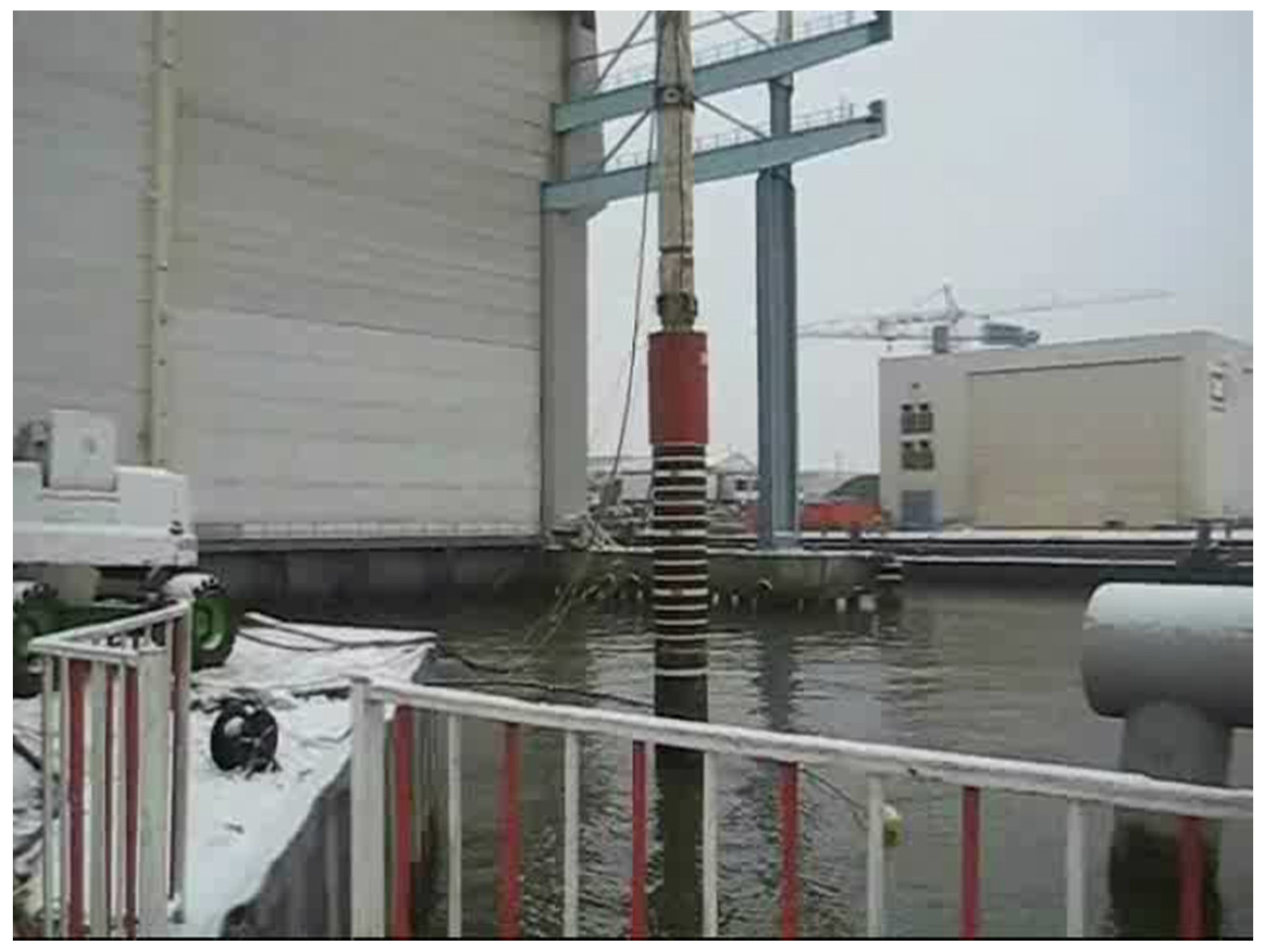
Tests made at Kinderdijk [
7] to study the mitigation of piling noise in the water, provided well controlled repeatable conditions, albeit different from those of many applications. The opportunity was taken to also measure sediment motion. The coupling of the geophones to the sediment was not ideal, and the amplitudes recorded are not deemed an accurate measure of the sediment motion, but the wave arrival times were clearly linked to the blows on the instrumented pile (
Figure 1), fitted with accelerometers.
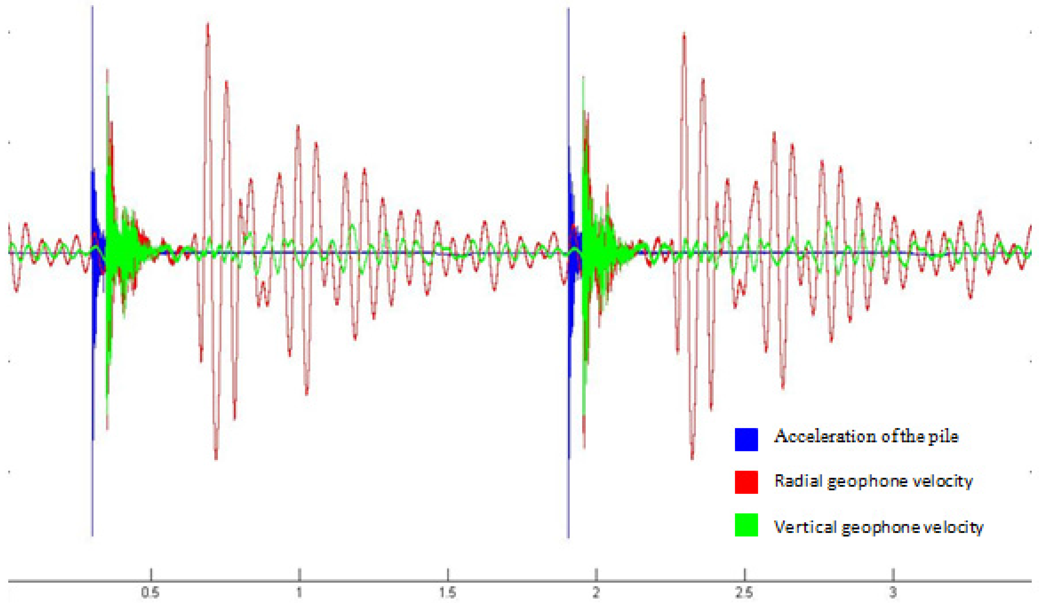
Figure 2 shows signals measured by geophones on the sledge, when set at 68 m from the pile, and aligned with its radiation direction. The time of each hammer blow was given by a pile acceleration signal (blue), which decays rapidly. About 45 ms later the geophones recorded a short high frequency pulse of similar duration, because the sledge housing provided some coupling to this pressure wave. After 350 ms a separate low frequency wave arrived, showing the orthogonal phase relation between the vertical and horizontal waveforms characteristic of a ground roll. Peak velocities ~2.5 mm/s were recorded by the horizontal geophone aligned to measure a radial wave velocity. However, the sledge only rested on the sediment, so the coupling between the sediment and the geophone was uncertain. Whilst the seismometer calibration covers frequencies to 200 Hz, it is not valid for the higher frequency water pressure waves, and only their timing has been used, as shown in the time series of
Figure 2, marked in seconds.
3. Modeling the Response by Finite Element (FE) Analysis
The results as shown in
Figure 2 have two distinct responses seen for every blow. Initially, reverberation was considered as an explanation, but then rejected due to the dramatic differences in the nature of the later arrival wave by comparison to the vibration within the pile itself and the earlier pressure wave.
Initial FE models started with the hammer, the steel pile, and the water, with some success in producing the early arrival pressure wave. The prediction of a conical wavefront within the water, subsequently described as a “Mach wave” by Reinhall and Dahl [
3] was confirmed by an analysis of the hydrophone array data. Each hammer blow produces a solid compression wave which travels rapidly down the pile, so that sound waves are radiated progressively from source points down the pile to follow a direction which depends on the ratio of the speed of these two waveforms.
Whilst a prediction of energy radiated into the water during the first passage of the compression wave within the pile could be made without any sediment data, subsequent activity depends on the reflection of this wave back up towards the hammer. The mechanics of the conversion of piling energy into the ground are difficult to predict. The necessity to include complex, time variant and nonlinear sediment properties led to a deferral of this aspect of the work, which is thus not reported here.
Whilst this obstacle was being considered, other information suggested that the later arrival was a sediment interface wave, for which the precise nature of the input deformation is not critical. This prompted a switch to modeling the measured sediment waves as seen in the data (
Figure 2). These waves were modeled without piling data, but with realistic sediment data taken from a review of many measurements by Hamilton [
9], adjusting the source waveforms to give the most easily understandable effects. A very short and simple wavelet has been generated, which keeps the energy concentrated, and thus delivers strong peak motions. The evident narrow frequency bands of both the measured data and the model output have a restricted relationship with the pile vibration waveforms and model source respectively, but are largely controlled by the filtration provided by the sediment structure.
An analogous response occurs for a bell struck by a hammer. The sounds radiated into the air depend primarily on the modal response of the bell structure, but with some variation of the distribution over different modes dependent on the nature of the blow. However, a bell’s vibration energy remains within its structure, whereas the sediment vibrations travel outwards as radiated energy. An individual seismometer in an array on the seabed will only register energy for the duration of the wavelet, with the energy being passed on toward the next sensor. Both the bell and the seabed act as filters, accepting impact energy preferentially at resonant frequencies. The investigation of the seabed wave can then be studied using an impact designed to excite the desired mode.
4. The Use of a Graded Layer Sediment Structure to Mimic the Narrow Band Results
It became clear that a graded layered sediment was needed to best replicate the observed measurements. The layered structure adopted for the response shown here is given in
Table 1. Wave speeds, Vs (shear) and Vp (pressure), were taken from Hamilton’s review data, and the 128 m depth of the model divided into eight layers. The Young’s modulus E, and Poisson ratio, ν, were calculated using a uniform density of 2250 kg/m
3 for this general study. Values of Vs increased from 117 m/s to 368 m/s, comparable with the data reviewed. No intrinsic absorption was included.
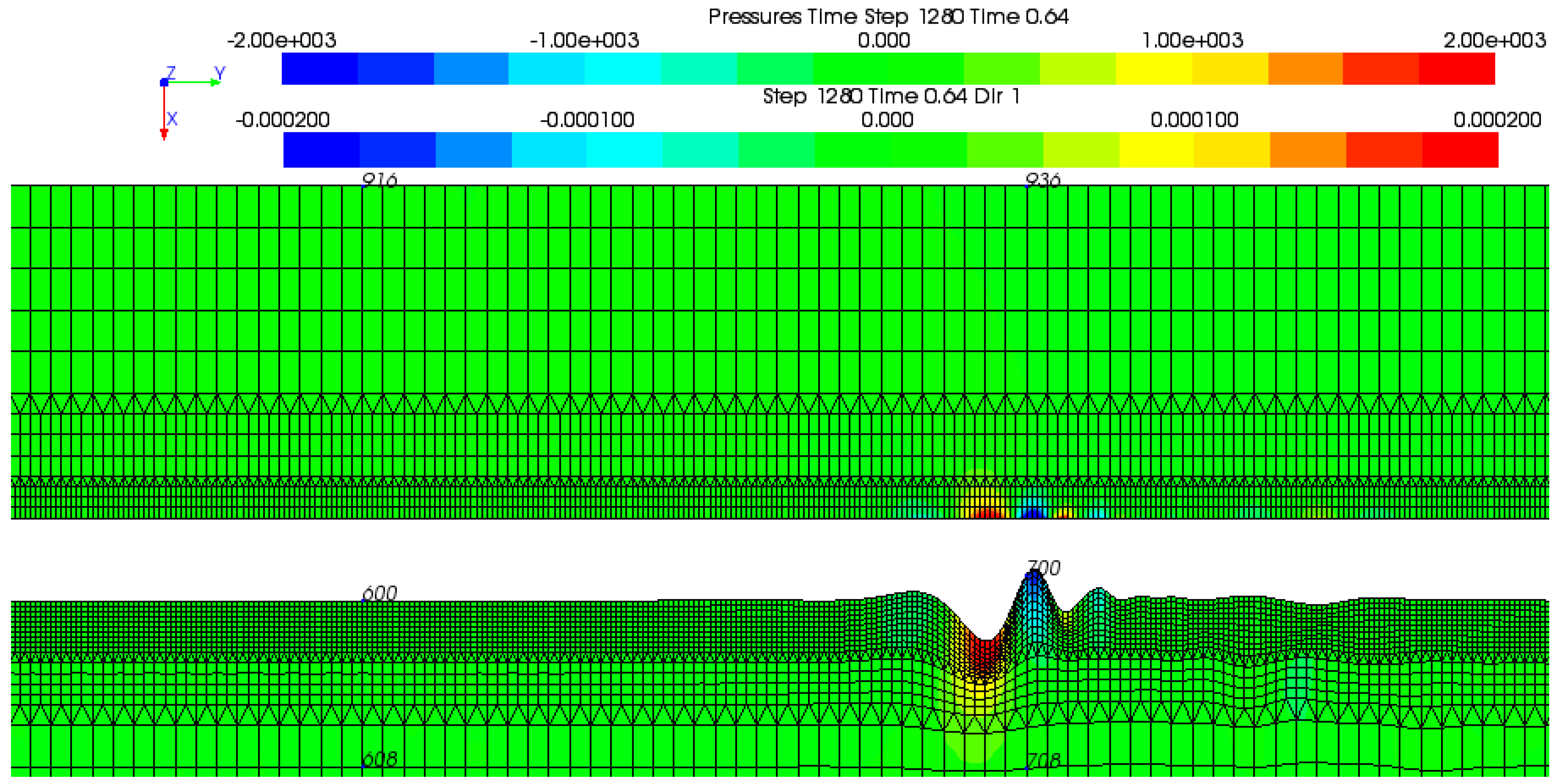
A downward force with an arbitrary 1 MN peak was applied to a point on the seabed, the origin of this axisymmetric model, which created water pressures >2 kPa at 32 m radius. A force time function,
MN, was used over a period (τ). This impulse was developed for other work by one author (PCM) to minimize high frequency content in a finite duration. A period τ = 40 ms created a short wavelet. Time steps (t) in this transient analysis (
Figure 3 and
Figure 4) were 0.5 ms.
Although these displays only show the response to 8 m depth within the sediment, the exponential reduction of motional displacement is displayed, and the green colouration continues to the 128 m base of the model. By changing the assignment of the false colours, the less intense waves radiated into the bulk can be seen, but these create little motion at depth.
Some of the finite elements are shown, structured to provide detail near the interface, whilst minimizing the run time by the use of larger elements elsewhere, down to 128 m. The smaller model elements near the interface are required for the slower wavespeeds, to satisfy the Courant condition. Model changes at depth had little effect, showing the results to be determined by the top sediment layers. The energy is also confined in frequency, centered on ~20 Hz for this mode, with a principal wavelength of ~5 m, and a wave speed close to 100 m/s, a little less than the shear speed at the seabed of the Hamilton profile, as expected. The initial vertical thrust generates a downward propagating wave which is rapidly refracted back to the seabed. This profiled velocity structure is highly selective, filtering the wide frequency range within realistic piling blows to accept energy which propagates in this wavelet form.
In animation (see
supplementary data) this progression can be seen in more detail, and the difference between group velocity and phase velocity can be seen to move the internal peaks and dips through the wavelet energy envelope.
5. Interface Waves in Layered Solid Seabeds—“Dispersive” versus “Nondispersive”
Waves confined to an interface such as the seabed, which are different from planar body waves, involve motion orthogonal to the propagation direction. They cannot occur in models which approximate solids as fluids as they are propagated by the shear stress.
Lord Rayleigh [
10] considered an interface, a division of space into two infinite “half spaces”, between an isotropic solid and a vacuum. “Rayleigh waves” can then move along a horizontal surface with their vertical and horizontal motions out of phase. For his simple model, they are non-dispersive, so any source waveform can be transmitted without distortion, a predictable property when no dimensions of length are specified [
11]. The wave speed is controlled by the solid’s shear modulus, its density, and Poisson ratio.
In contrast, waves in layered structures are usually dispersive, because reflections between multiple interfaces affect their speed, making this a function of frequency. But as has been recorded by Schmalfeldt and Rauch [
12], wavelets propagated along the seabed after an explosion show modal properties. These seismic wavelets bear little relationship to the source waveform, but the waves can be detected after travelling distances measured in kilometers. Jensen et al. [
13] compare their data with models made by wavenumber integration, to provide confirmation of the graded seabed structures reported by Hamilton [
9]. Since this technique is in some ways complementary to FEA, more detailed comparisons may prove useful. Both can study the water particle velocities believed important for biological studies (Hovem and Korakas [
14]).
The nomenclature in this field may be in need of revision, as many authors after Rayleigh have developed it. Substantial work by Strick et al. [
15], discussed the extension of the “true Rayleigh wave” model, first by Stoneley [
16] and then Scholte [
17], who substituted different isotropic materials for the vacuum. Strick also described a “pseudo-Rayleigh wave”, but in a footnote (p. 487) found the “nomenclature to be in need of revision”. The distinction between dispersive and non-dispersive waves is often not made clear, and is important if communications applications are being considered. Information is often carried by modulation, and the strong filtration of ground roll waveforms makes this difficult.
All these wave types show a phase quadrature motion described by seismologists as ground roll [
18]. The particle displacements can be presented as hodographs, which display their elliptical motion. But the layer thicknesses of a graded solid seabed change the wide band response of a non-dispersive isotropic medium to a strong filter action which creates the modal structure. Achenbach [
11] points out that Stoneley waves are non-dispersive, occurring for a half space interface between two different solids, or between a solid and a fluid as discussed by van Dalen et al. [
19]. However Yilmaz [
18] describes ground roll as “dispersive surface waves”.
This descriptive term “ground roll” has been used in presentations [
20] for interface waves where the elliptical motion is the common feature. An analogous usage is that of the “rolling ocean waves” where the water near the surface moves in circles of decreasing diameter with depth. This motion is also analogous to a manual polishing action, which is circular but irrotational, in contrast to the rotary motion of a polishing machine. Irrotational motions avoid the energy losses associated with vortices.
6. Lower Frequency Modes and Wavenumber Integration Models
Other modes exist in reality, described by Jensen et al. [
13]. Their results, filtered for frequencies below 10 Hz [
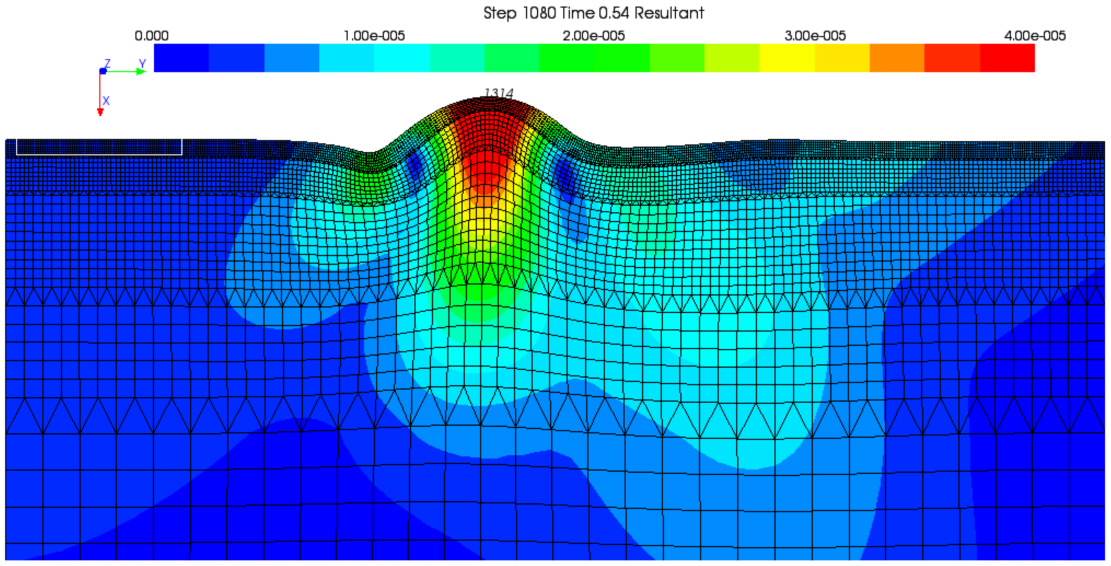
12] showed modes at ~3 Hz which propagated to well over 1 km range, generated by seabed explosions. The wavenumber integration modeling by Jensen et al. was also able to predict absorption by a best fit procedure of the model damping. A ~5 Hz mode was generated in our FEA structure (model HLL1) by increasing the period of the source waveform As expected the longer wavelength 5 Hz wave is seen to penetrate deeper into the seabed (
Figure 5).
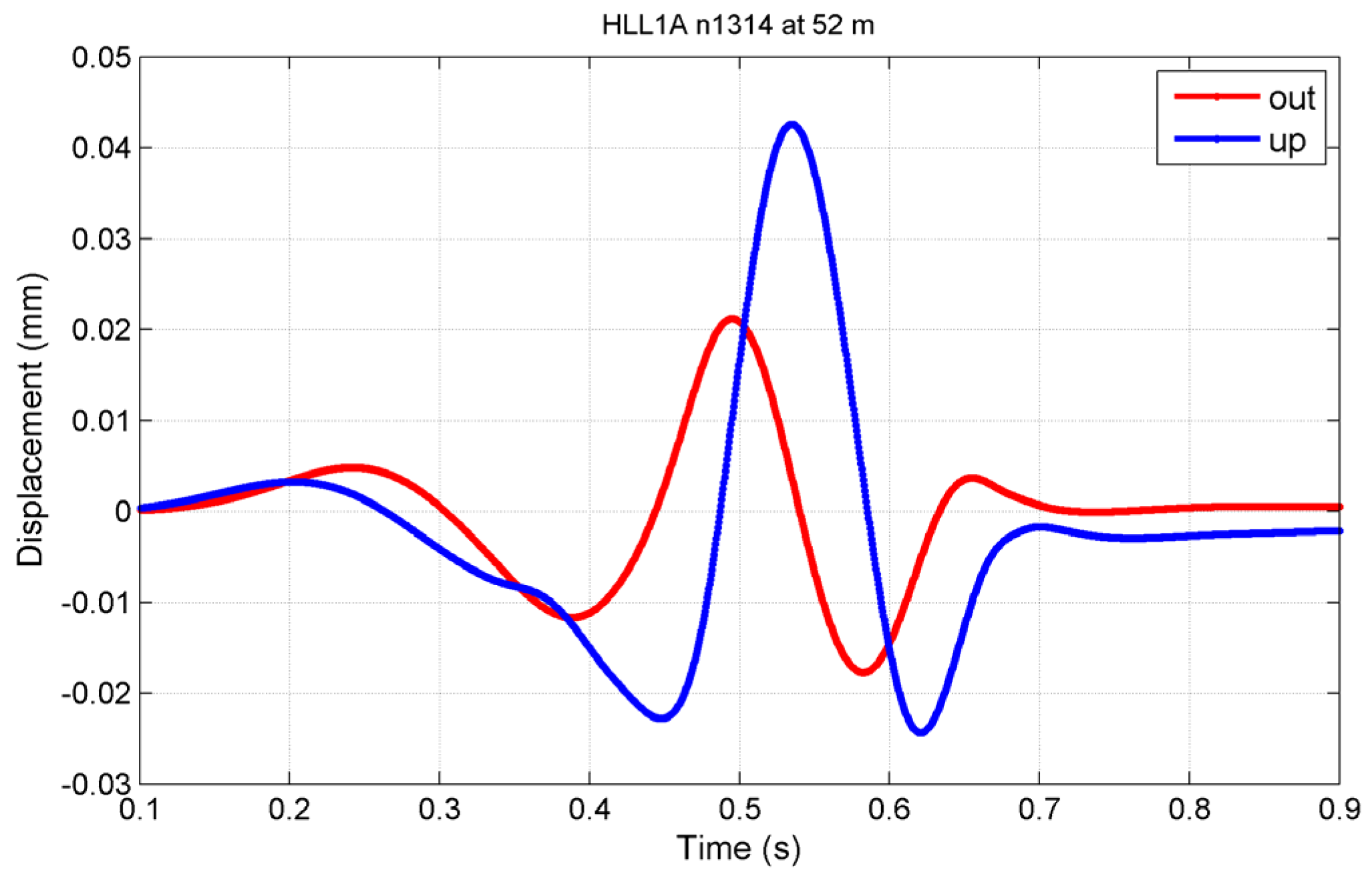
Analysis of the motion in
Figure 6 shows the dominant frequency to be ~5 Hz, driven by a 0.2 s long forcing function. The upward motion peaks at just over 40 μm for the arbitrary 1 MN peak downward force. The upward motion is in phase quadrature with the outward motion which peaks when the vertical motion is zero. This feature is the key property of the ground roll motion shared by Rayleigh, Stoneley and Scholte waves [
20].
More recent measurements by Reimann et al. [
6] were reported at a conference in Rhodes in June 2014, taken from a more comprehensive study in open water with multiple stations in the near and far field. They recorded peak pressures over 1 kPa and short wavelets of a comparable nature to those shown here.
7. Details of the Solid Motion—The Transition from Retrograde to Prograde
The 20 Hz mode was analysed (
Figure 7 and
Figure 8) using a sequence of nodes with depth seen in
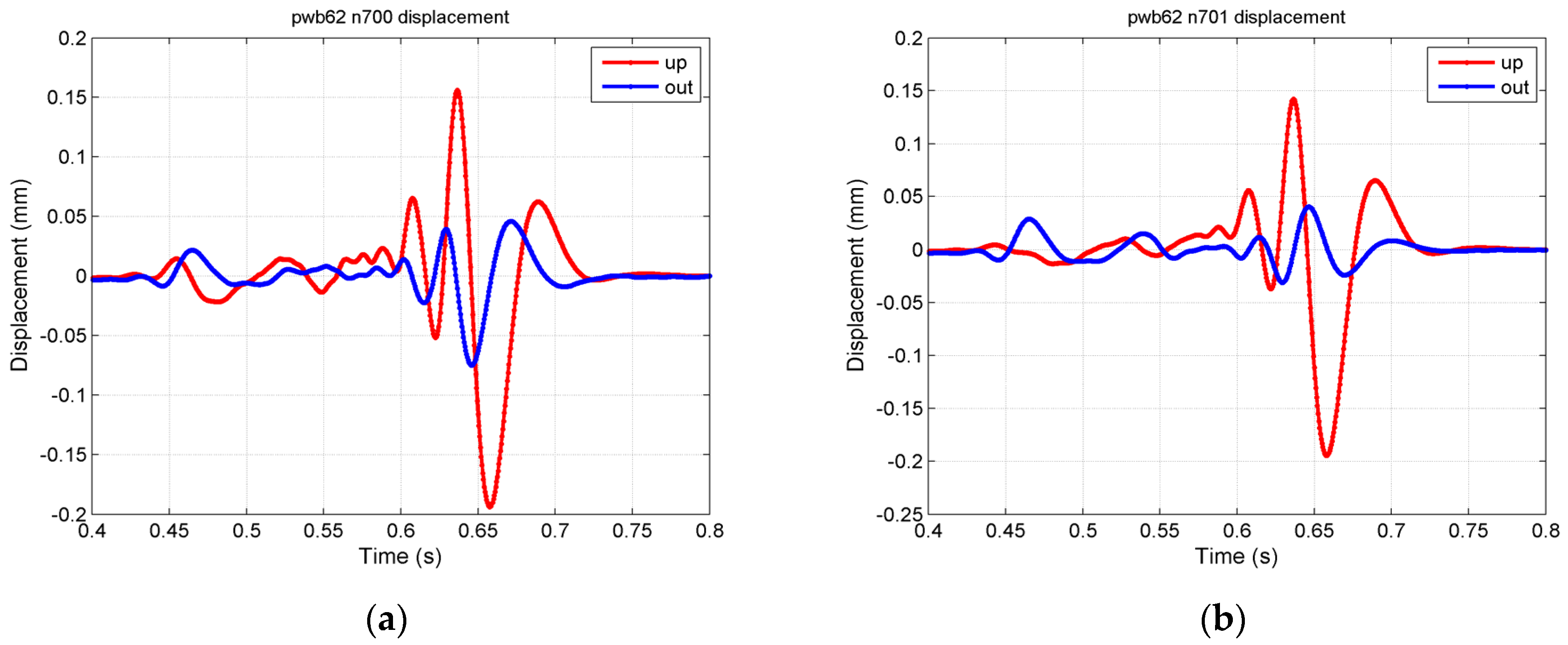
Figure 9 at 64 m range. Particle displacements at nodes 700 and 701 show a strong dip which develops just after 0.64 s.
At the seabed, node 700, the horizontal displacement of the solid, outward from the origin, changes from negative to positive during the dip. The seabed thus moves with the direction of propagation during a dip, but against it when at a hump. This is described as a retrograde motion. However at 1 m depth (node 701) there is a reversal to a prograde motion, and the transition depth of this reversal lies between 0 and 1 m below the seabed. The vertical motion barely changes but the horizontal displacement becomes smaller and is inverted in phase.
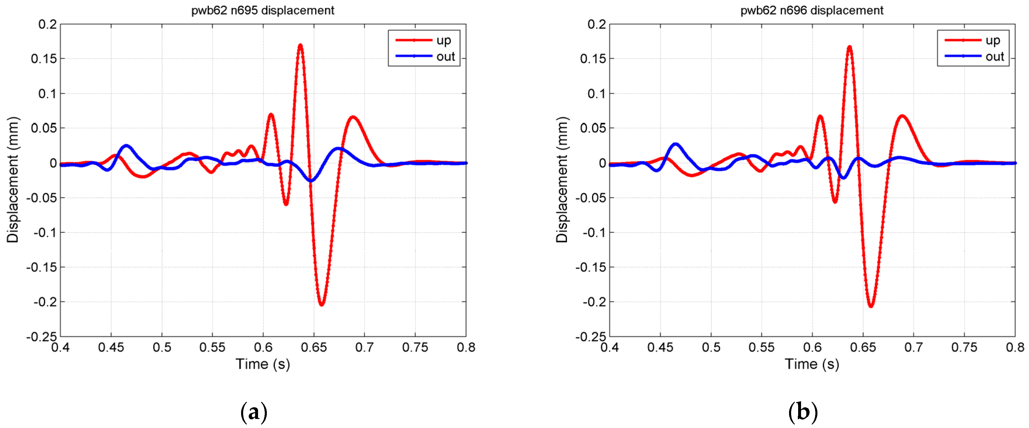
Extra nodes between n700 and n701 show the varying horizontal motion to greater resolution. The transition depth lies between nodes 695 (0.25 m depth) and 696 (0.5 m depth). A depth of 40 cm is estimated by interpolation.
8. The Distribution of Stress
The propagation of the wave requires an exchange of energy between that stored as elastic stress and that stored as kinetic energy. Plots of solid shear stress and displacement display this.
A feature of the wave shown in
Figure 9 is the concentration of shear stress, σ
xy, either side of a minimum. The two red areas have opposite sign shear stresses, with a central minimum where the upward displacements (in the direction of negative ×) are at a maximum (
Figure 10). Both shear stress peaks lie below the transition depth, showing that shear energy is concentrated in the prograde region. There is a contrast between the distribution of stress and that of displacement (and velocity). Whilst the vertical displacements peak below the 0.4 m transition depth, they are also large above this transition depth, so that the kinetic energy concentration covers both the retrograde and the prograde regions.
9. Details of the Water Motion—Linking Pressures to Velocity and Acceleration
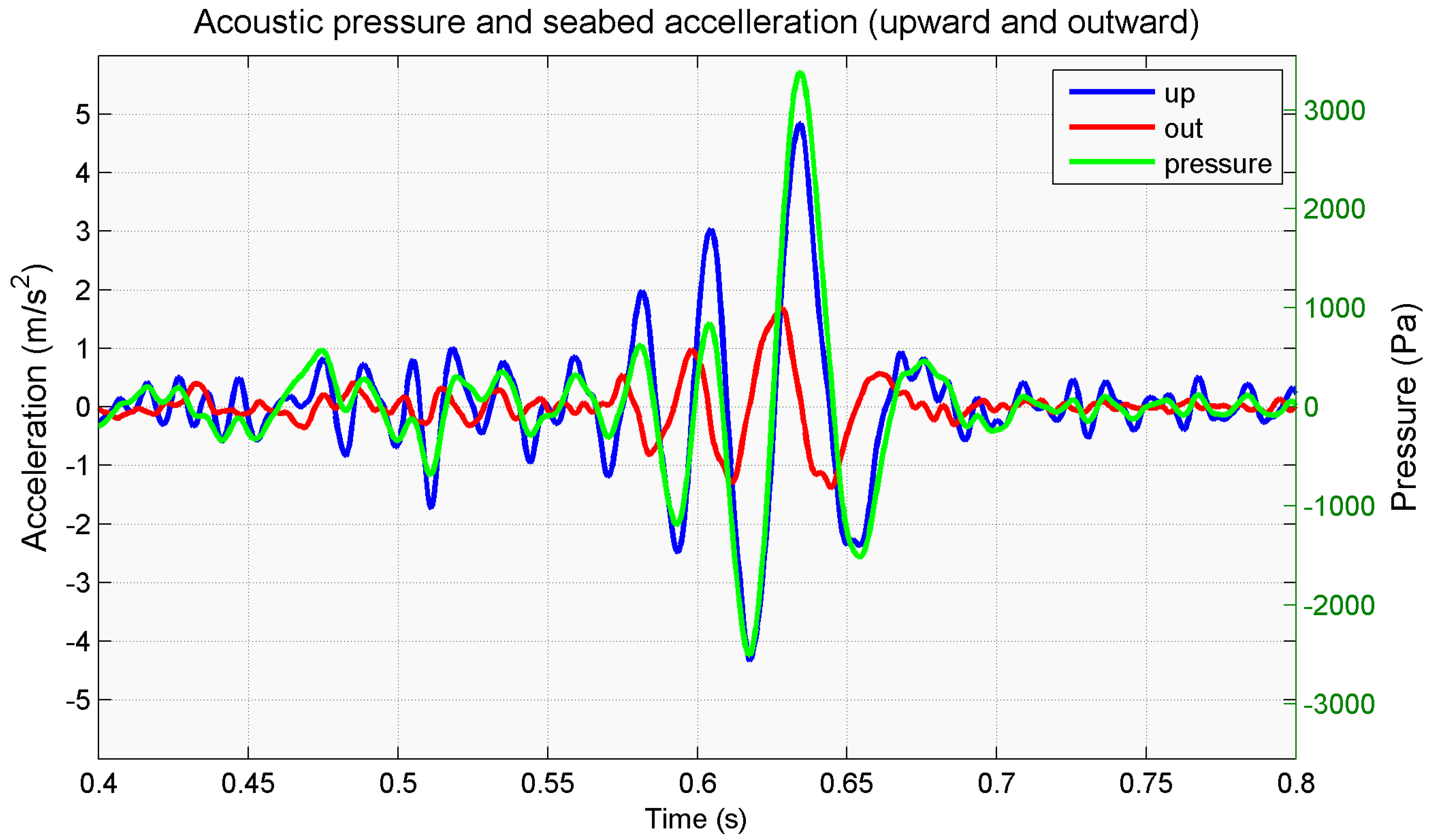
Figure 11 shows the similarity in waveform between the acceleration and acoustic pressure at the interface. Fluid node 8394 is co-located with solid node 700. The minimal phase shift shows that the pressures are linked to the acceleration in a Newtonian manner. This contrasts with the plane wave case, where it is the water velocity which is in phase with the pressure. The usual acoustic impedance has become complex, with a phase change of ~π/2 radians. The ratio of pressure P to vertical velocity V for the 20 Hz component can be assessed from this data as ~75,000 Pa/(m/s). The P/V ratio (acoustic impedance) for planar pressure waves in sea water is ~1.5 MPa/(m/s). The magnitudes of these ratios differ by a factor 20, showing that the vertical water velocities are much larger than might be expected from a pressure measurement at that point. As will be shown, the horizontal velocity components in the water near the interface are comparable.
This seismic wavelet is small compared with the wavelength of a pressure wave in water (~75 m for a 20 Hz wave). This change in relation between P and V is also seen when close to a small variable volume source in bulk media, that is, within the “near field” of a “simple source” [
21].
10. Large Horizontal Water Motion Occurs over Ground Roll
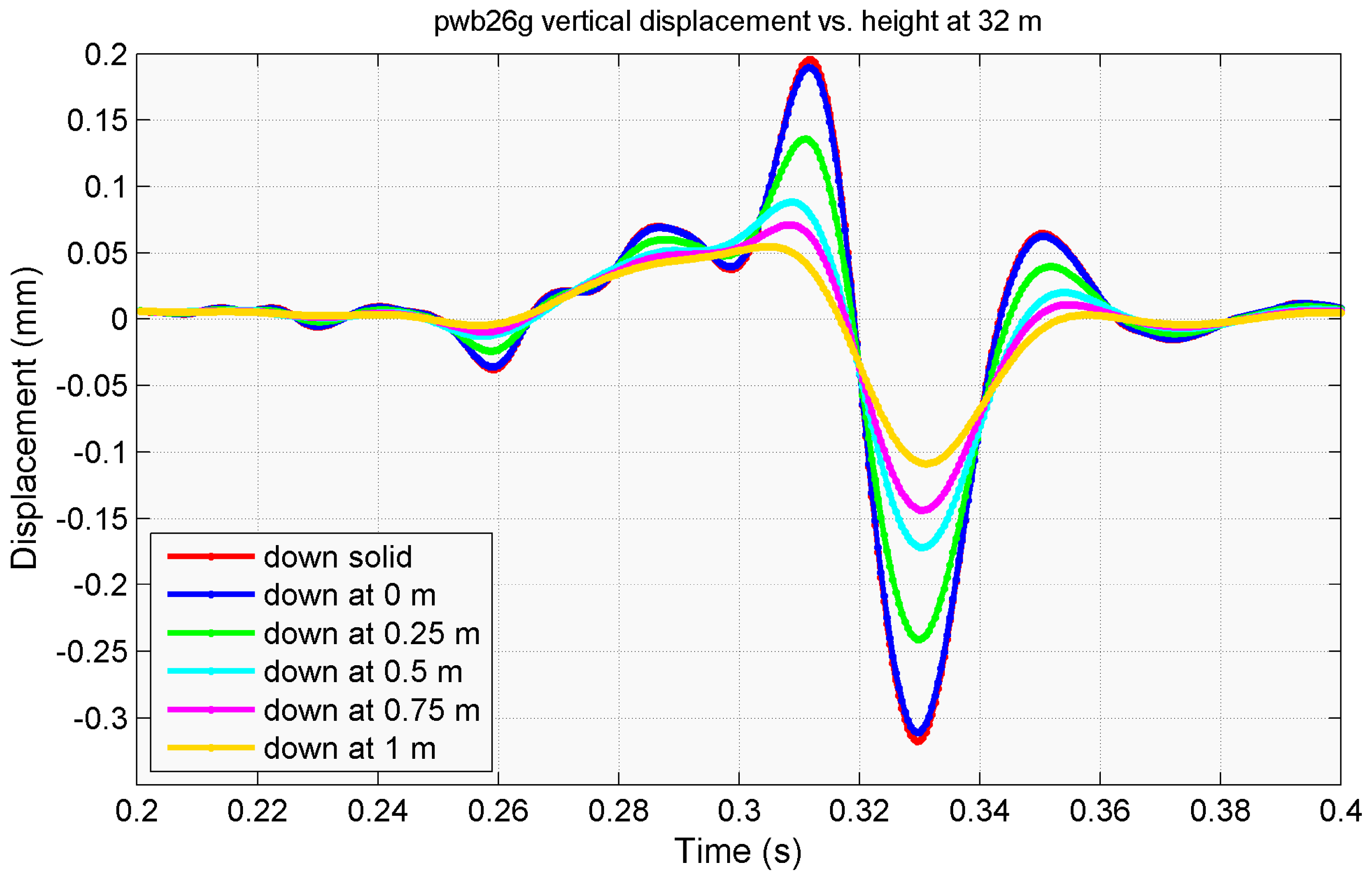
An evanescent decay with height occurs both for the pressures, and for vertical displacement, shown in
Figure 12 using data from 5 fluid nodes up to 1 m above the seabed. Data from the co-located solid (red trace) and fluid node at 0 m above the seabed (blue trace) agree closely as expected.
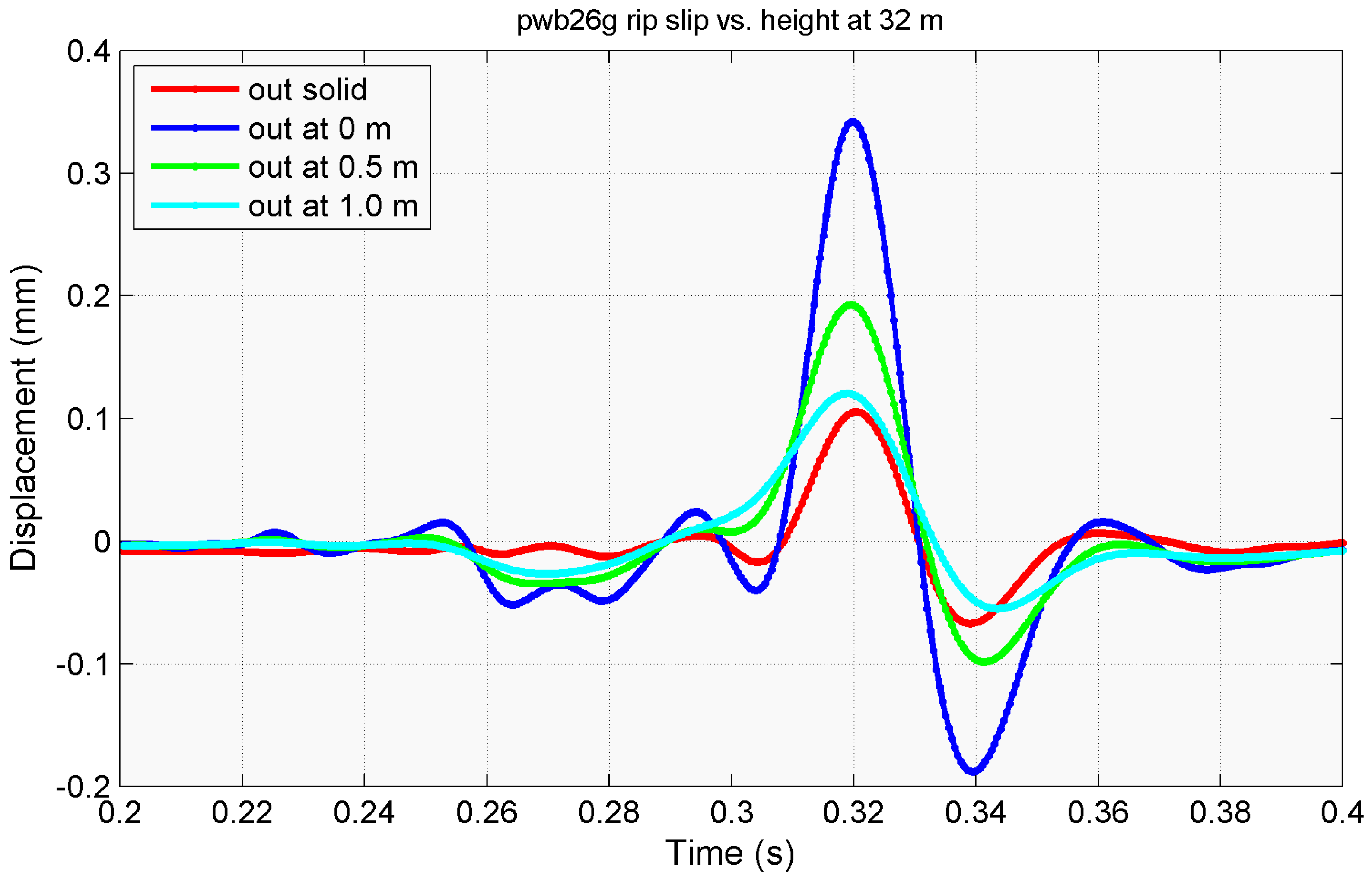
In contrast, the radial (outward) motions (
Figure 13) show a differential horizontal motion between the water and the seabed which it at a maximum for the adjacent water node. The model imposes no mechanical restraint on such motion at the interface. This slippage between the adjacent water and the seabed will apply ripping forces to any structure which extends across this interface, such as filter feeding shellfish. This phenomenon has been described as a “rip-slip” action in past presentations. The prediction has not been experimentally tested but such work may be undertaken.
In practice there will be a boundary layer in which there will be a velocity gradient. Whilst this is not covered by the FE modeling the layer is likely to be thin, much less than the element size, with minimal effects on their motion. There is no account taken here of any boundary layer turbulence, as the water slides briefly across the sediment. However, estimated Reynold’s numbers are small, of the order of 100 (using the kinematic viscosity ν of water ≈ 1 × 10⁻⁶ m2/s, velocities ~1 mm/s, and dimensions ~0.1 m) so the slippage is unlikely to generate turbulence.
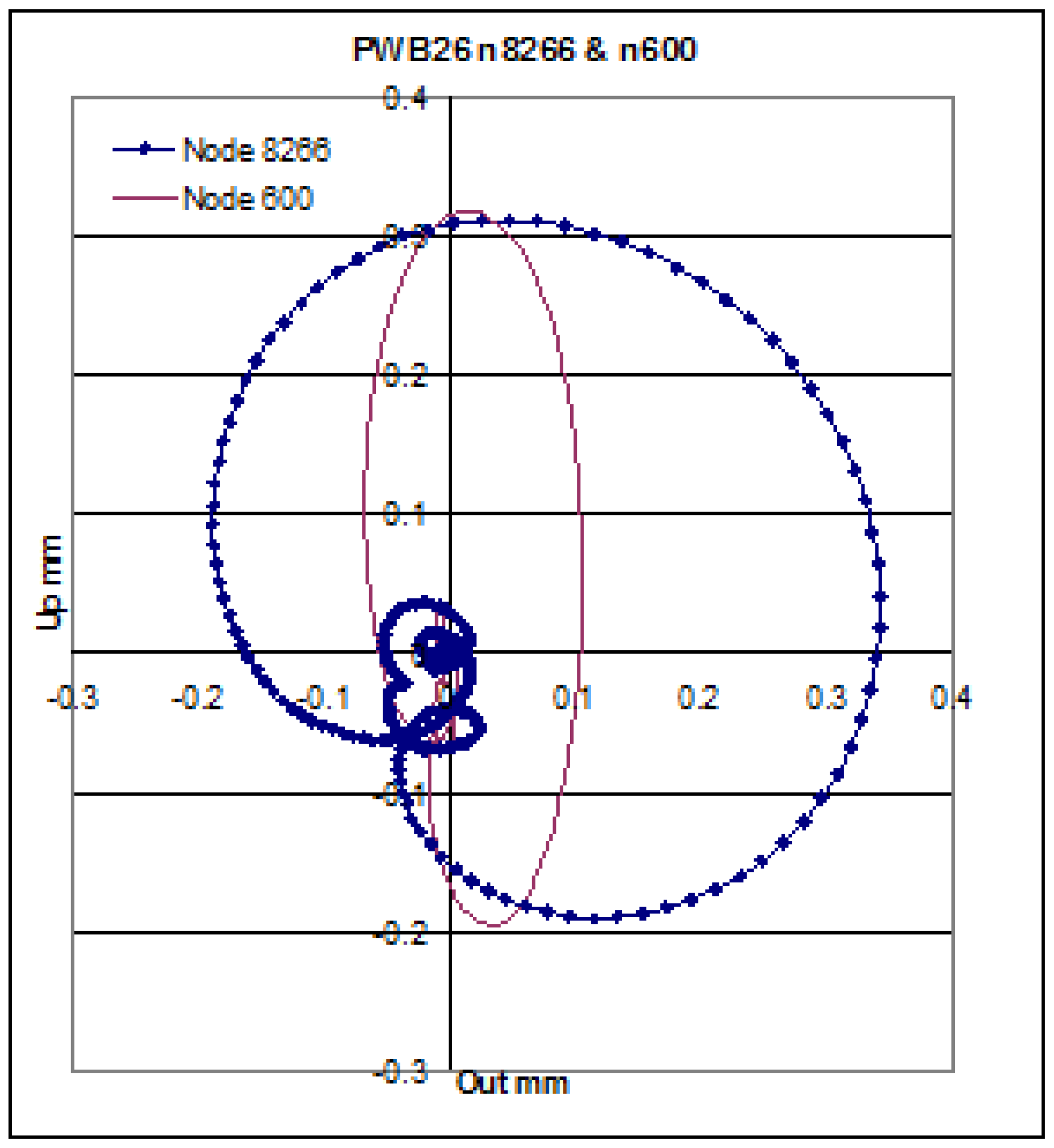
The rip-slip action is clearly seen in the hodograph of
Figure 14, where the upward displacement is plotted against the radial outward displacement. Model results for individual time steps (0.5 ms) of the transient analysis show anticlockwise water motion represented by node 8266. This forms an almost circular or cardioid shape in contrast to the more constrained elliptical motion of the seabed, at the co-located node 600. Both sequences start and finish near the origin, but the individual steps are not shown for the motion of solid node 600 for clarity.
11. The Extra Information in the Vector Field May be Critical for Benthic Species
Acoustic pressure gives a scalar field, providing directional ambiguities for sensors which are small compared to the wavelength. Kotas et al. [
22] and Webb et al. [
23] describe the “180 deg ambiguity” which remains for plane waves, even when the “line of bearing” can be determined by using their otolith inertial sensors. Klages et al. [
24] consider how “micro seismic events” such as food falling onto the deep seabed may provide critical information for benthic species. They cite work on the sensitivity of crustaceans to any particle displacement amplitudes (PDA) over 0.1 μm and cite references to PDA thresholds at around 80 Hz of well below 0.01 μm for lobsters. This corresponds to water particle velocities of only 5 μm/s.
In contrast to pressure waves, the water motion driven by ground roll has components orthogonal to the propagation direction. The successive points in
Figure 14 are anticlockwise, a retrograde direction of roll, where the horizontal velocity at the top of the loop opposes the direction of energy flow. If this roll direction can be detected by small creatures they may find it useful to determine which way to hunt or flee. As was discussed by Hazelwood & Macey [
25] this is feasible for creatures with 3 axis inertial sensors, even when small by comparison to a wavelength.
12. Conclusions
The motions induced in the overlying water by seismic interface waves have been studied as a potential influence on aquatic life. The additional information provided by these low frequency waves may help creatures determine the directions to hunt or flee. Even immobile creatures may have their feeding inhibited by the rip-slip action as the water slides to and fro across the seabed. The nature of seismic waves produced by man-made impacts on the seabed have been studied in detail to provide information which should help in future research. Various predictions made by the study are amenable to practical tests which if confirmed would help explain how small benthic creatures can function, both as predators and as prey.
Acknowledgments
The test pile at Kinderdijk was operated by IHC Hydrohammer BV. Data collection and help with analysis was made by TNO Delft The Netherlands, especially Erwin Jansen. Further analysis was conducted with the help of Stephen Robinson of the National Physical Laboratory, Teddington, UK, (NPL). Supporting data from the dredger trial was provided by NPL. Encouragement to venture into biological matters was provided by Tony Hawkins, and research data provided by Louise Roberts.
Author Contributions
The modelling work was collaborative but the measurements were made by Richard A Hazelwood. Patrick C Macey specializes in acoustically coupled modeling
Conflicts of Interest
The authors declare no conflict of interest.
References
- Thomsen, F.; Gill, A.; Kosecka, M.; Andersson, M.; Andre, M.; Degraer, S.; Folegot, T.; Gabriel, J.; Judd, A.; Neumann, T.; et al. MaRVEN—Environmental Impacts of Noise, Vibrations and Electromagnetic Emissions from Marine Renewable Energy; Final Study Report of Project RTD-KI-NA-27-738-EN-N, EUR 27738; European Commission: Brussels, Belgium, September 2015. [Google Scholar]
- Popper, A.N.; Hawkins, A.D.; Fay, R.R.; Mann, D.A.; Bartol, S.; Carlson, T.J.; Coombs, S.; Ellison, W.T.; Gentry, R.L.; Halvorsen, M.B.; et al. Sound Exposure Guidelines for Fishes and Sea Turtles; ASA S3/SC1.4 TR-2014, Technical Report by ANSI- Standards Committee S3/SC1, ISSN 2196-1212; Springer: New York, NY, USA, 2014. [Google Scholar]
- Reinhall, P.G.; Dahl, P.H. Underwater Mach wave radiation from impact pile driving: Theory and observation. J. Acoust. Soc. Am. 2011, 130, 1209–1216. [Google Scholar] [CrossRef] [PubMed]
- Zampolli, M.; Nijhof, M.J.J.; de Jong, C.A.F.; Ainslie, M.A.A.; Jansen, E.H.W.; Quesson, B.A.J. Validation of finite element computations for the quantitative prediction of underwater noise from impact pile driving. J. Acoust. Soc. Am. 2013, 133, 72–81. [Google Scholar] [CrossRef] [PubMed]
- Lippert, T.; von Estorff, O. The significance of parameter uncertainties for the prediction of offshore pile driving noise. J. Acoust. Soc. Am. 2014, 136, 2463–2471. [Google Scholar] [CrossRef] [PubMed]
- Reimann, K.; Grabe, J. Soil vibration due to offshore pile driving and induced underwater noise. In Proceedings of the UA2014—2nd International Conference and Exhibition on Underwater Acoustics, Rhodes, Greece, 6 July 2014; pp. 279–286.
- Jansen, H.W.; de Jong, C.A.F.; Middeldorp, F.M. Measurement Results of the Underwater Piling Experiment at Kinderdijk; Tech. Rep. RPT-DTS-2011-00546; TNO: Delft, The Netherlands, 2011. [Google Scholar]
- Robinson, S.P.; Theobald, P.D.; Hayman, G.; Wang, L.S.; Lepper, P.A.; Humphrey, V.; Mumford, S. Measurement of noise arising from marine aggregate dredging operations. In Marine Aggregates Levy Sustainability Fund report; MEPF Ref no 09/P108; MALSF: Southampton, UK, February 2011. [Google Scholar]
- Hamilton, E.L. Vp/Vs and Poisson’s ratio in marine sediments and rocks. J. Acoustic. Soc. Am. 1979, 66, 1093–1101. [Google Scholar] [CrossRef]
- Rayleigh, L. Interface waves. Proc. London Math. Soc. 1887, 17, 4–11. [Google Scholar]
- Achenbach, J.D. Wave Propagation in Elastic Solids; Elsevier Science B.V.: Amsterdam, The Netherlands, 1975; pp. 194–195. [Google Scholar]
- Schmalfeldt, B.; Rauch, D. Explosion-Generated Seismic Interface Waves in Shallow Water; Rep SR-71; SACLANT Undersea Research Center: La Spezia, Italy, 1983. [Google Scholar]
- Jensen, F.B.; Kuperman, W.A.; Porter, M.B.; Schmidt, H. Computational Ocean Acoustics; Springer-Verlag: New York, NY, USA, 2000; pp. 471–477. [Google Scholar]
- Hovem, J.M.; Korakas, A. Modeling low frequency propagation loss in the oceans. In Proceedings of the 1st Underwater Acoustics Conference, Corfu, Greece, 23–28 June 2013; pp. 1517–1522.
- Strick, E.; Roever, W.L.; Vining, T.L. Propagation of elastic wave motion from an impulsive source along a fluid/solid interface. Proc. Royal Soc. A 1959, 251, 455–523. [Google Scholar]
- Stoneley, R. Elastic waves at the surface of separation of two solids. Proc. Royal Soc. A 1924, 106, 416–428. [Google Scholar] [CrossRef]
- Scholte, J.G. On true and pseudo Rayleigh waves. Proc. Kon. Ned. Akad. Wetensch. Amst. 1949, 52, 652–653. [Google Scholar]
- Yilmaz, O. Seismic Data Processing; Soc. Exploration Geophysicists: Tulsa, OK, USA, 1987; pp. 40–42. [Google Scholar]
- Van Dalen, K.N.; Drijkoningen, G.G.; Smeulders, D.M.; Heller, H.K. Medium characterization from interface-wave impedance and ellipticity. J. Acoust. Soc. Am. 2011, 130, 1299–1312. [Google Scholar] [CrossRef] [PubMed]
- Hazelwood, R.A. Ground roll waves as a potential influence on fish. In The Effects of Noise on Aquatic Life; Popper, A.N., Hawkins, A.D., Eds.; Springer Science+Business Media: New York, NY, USA, 2012; pp. 449–452. [Google Scholar]
- Kinsler, L.E. Fundamentals of Acoustics; John Wiley & Sons: New York, NY, USA, 1982. [Google Scholar]
- Kotas, C.W.; Rogers, P.H.; Yoda, M. Acoustically induced streaming flows near a model cod otolith and their potential implications for fish hearing. J. Acoust. Soc. Am. 2011, 130, 1049–1059. [Google Scholar] [CrossRef] [PubMed]
- Webb, J.F.; Popper, A.N.; Fay, R.R. (Eds.) Fish Bioacoustics; Springer Science+Business Media: New York, NY, USA, 2008.
- Klages, M.; Muyaskin, S.; Soltwedel, T.; Arntz, W. Mechanoreption, a possible mechanism for food fall detection in deep-sea scavengers. Deep-Sea Res. Part I 2002, 49, 143–155. [Google Scholar] [CrossRef]
- Hazelwood, R.A.; Macey, P.C. The intrinsic directional information of ground roll waves. In The Effects of Noise on Aquatic Life II; Popper, A.N., Hawkins, A.D., Eds.; Springer: New York, NY, USA, 2016. [Google Scholar]
Figure 1.
The test pile of IHC Hydrohammer B.V. at Kinderdijk, near Rotterdam, The Netherlands. Hydrophones and geophones were deployed, connected to recording equipment on the quayside.
Figure 1.
The test pile of IHC Hydrohammer B.V. at Kinderdijk, near Rotterdam, The Netherlands. Hydrophones and geophones were deployed, connected to recording equipment on the quayside.
Figure 2.
Geophone and accelerometer time series signals for 70 kJ blows repeated every 1.6 s.
Figure 2.
Geophone and accelerometer time series signals for 70 kJ blows repeated every 1.6 s.
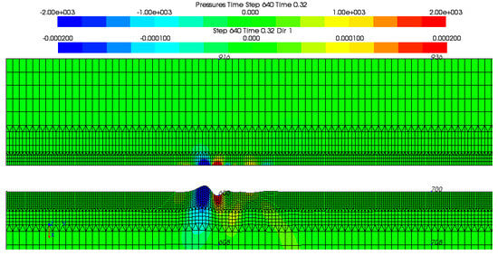
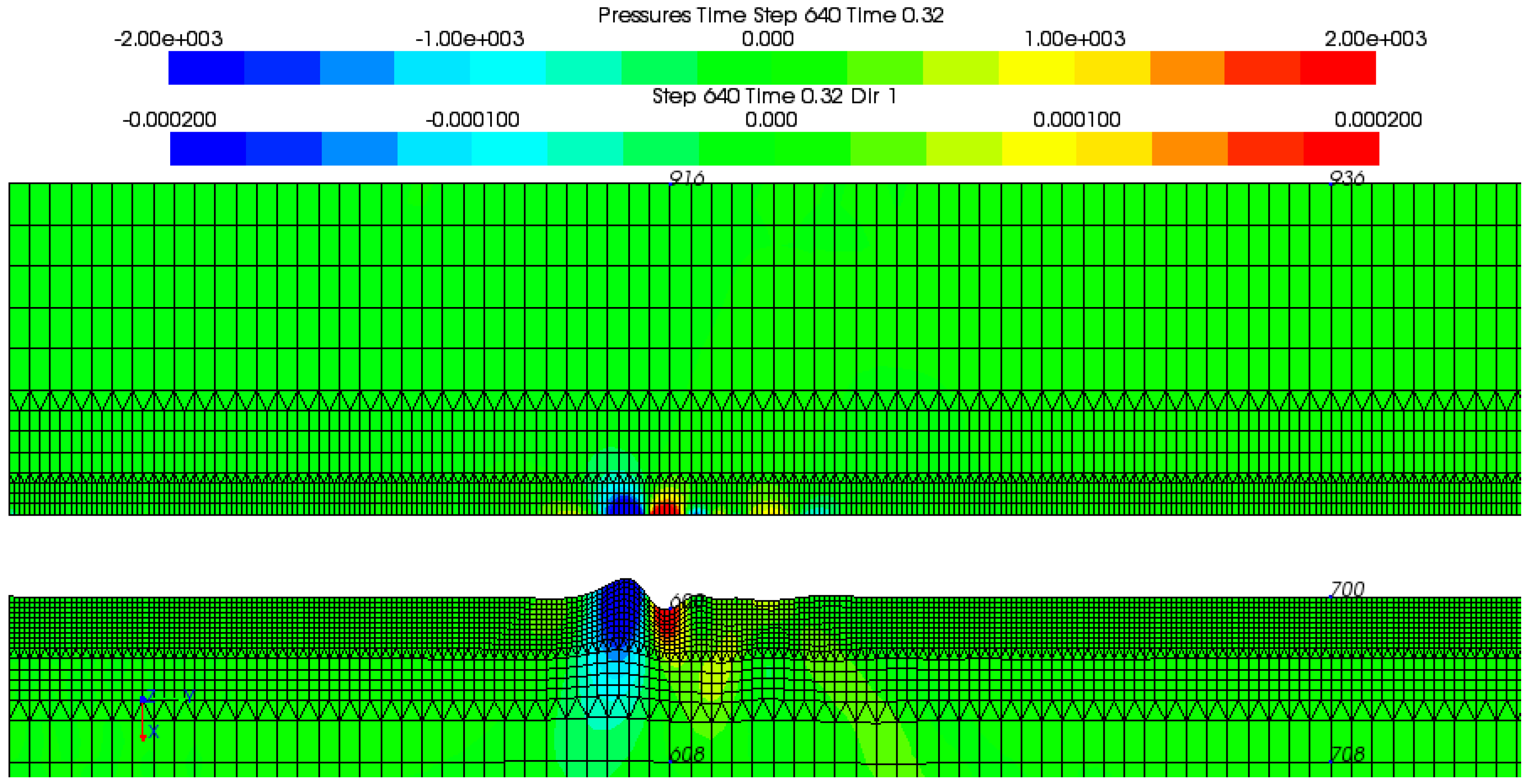
Figure 3.
A wavelet is shown at 0.32 s after the impact, 30 m from the source at the symmetry axis, on the left side. The white gap between the 16 m deep water and the underlying sediment is for clarity, showing its exaggerated deformation. Six nodes are shown, #600 at 32 m radius on the seabed, #916 m on the sea surface above, and #608 at 8 m below, plus #700, #708 and #936 at 64 m radius. The water pressures are indicated by the upper bar and vertical solid displacements by the lower bar.
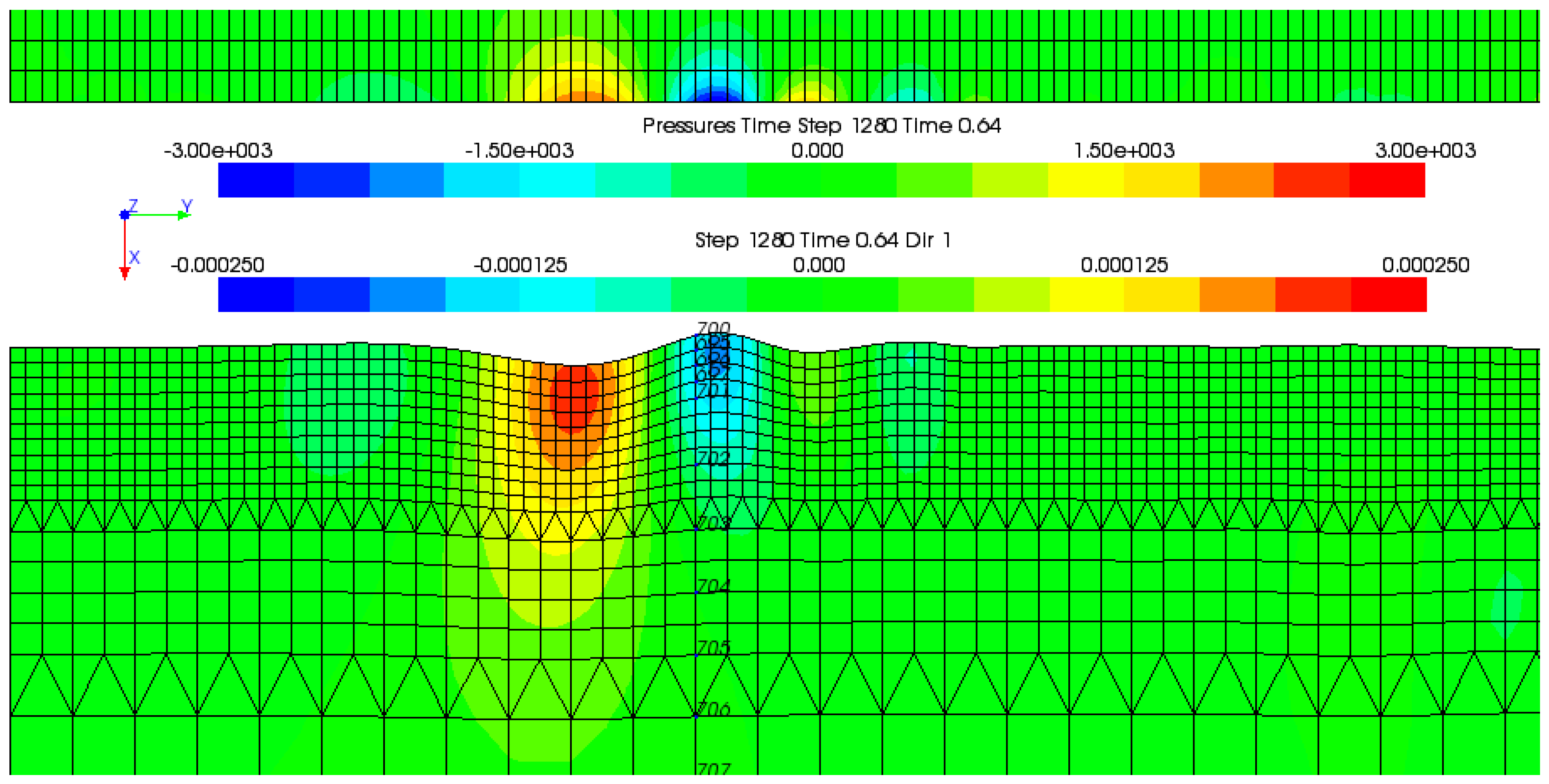
Figure 4.
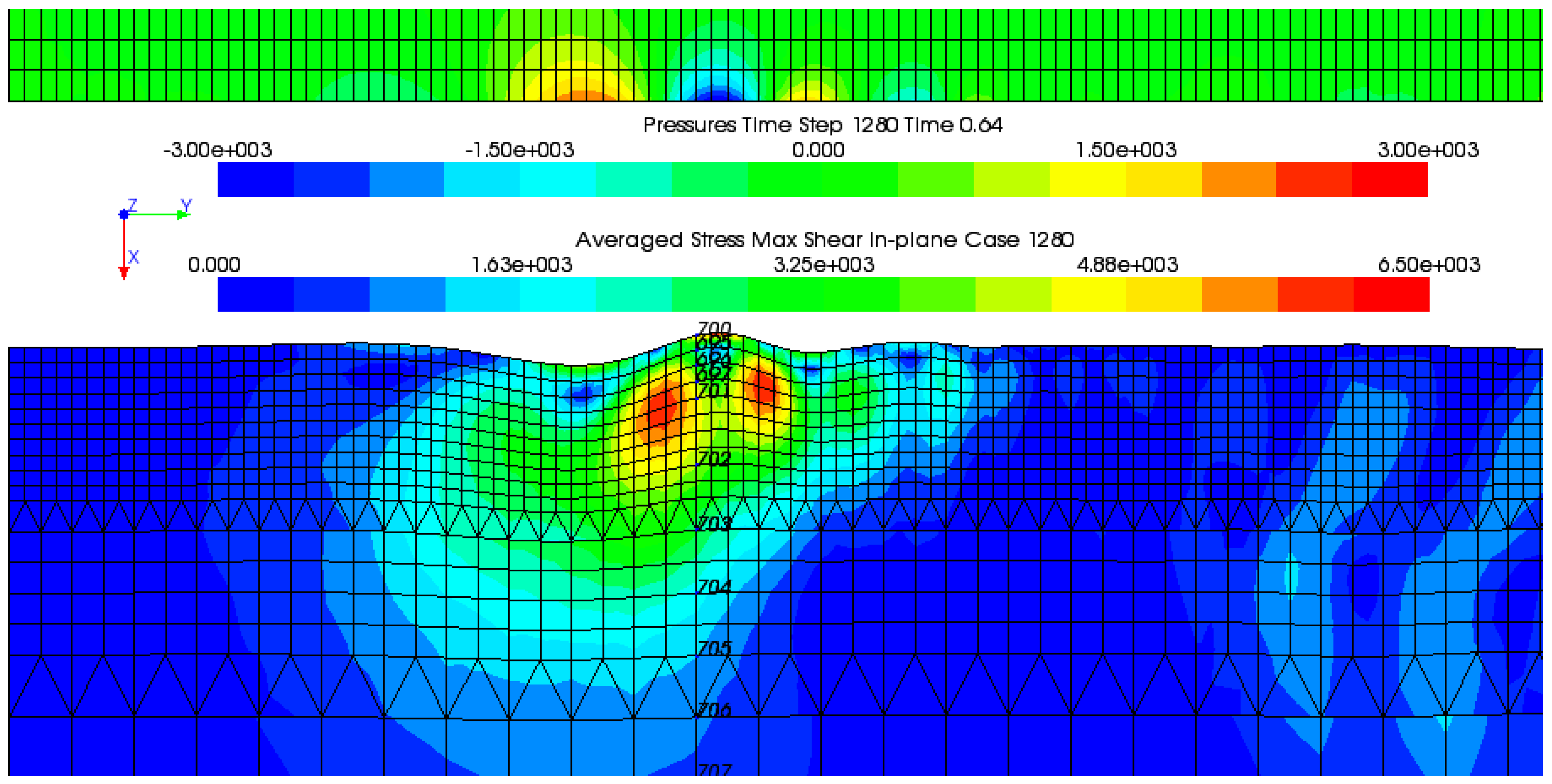
The wavelet is shown 0.64 s after the impact, at 64 m range (nodes 700 & 936). Whilst remaining compact, it has changed from a hump to a dip. The vertical (shown as × axis) sediment displacement shows a dip of >0.2 mm, creating a local peak pressure (>2 kPa) in the water.
Figure 4.
The wavelet is shown 0.64 s after the impact, at 64 m range (nodes 700 & 936). Whilst remaining compact, it has changed from a hump to a dip. The vertical (shown as × axis) sediment displacement shows a dip of >0.2 mm, creating a local peak pressure (>2 kPa) in the water.
Figure 5.
Model HLL1, with greater range but reduced mesh density is driven at ~5 Hz. A “hump” arrives at node 1314 at 52 m range after 0.54 s, shown as a displacement vector magnitude (low intensity becomes blue rather than green). At this moment it shows similarity to the Ricker or “Mexican hat” form.
Figure 6.
A time series of upward and outward motions at node 1314.
Figure 6.
A time series of upward and outward motions at node 1314.
Figure 7.
(a) A time series of motion at node 700; (b) Motion at node 701, 1 m below the seabed.
Figure 7.
(a) A time series of motion at node 700; (b) Motion at node 701, 1 m below the seabed.
Figure 8.
(a) Node 695 is at 0.25 m depth; (b) Node 696 is at 0.5 m depth.
Figure 8.
(a) Node 695 is at 0.25 m depth; (b) Node 696 is at 0.5 m depth.
Figure 9.
This enlarged view shows the shear stress magnitude, a measure of deformation.
Figure 9.
This enlarged view shows the shear stress magnitude, a measure of deformation.
Figure 10.
Vertical displacements deform the shape of the solid finite elements, storing energy.
Figure 10.
Vertical displacements deform the shape of the solid finite elements, storing energy.
Figure 11.
A time series of motion and acoustic pressure at the interface.
Figure 11.
A time series of motion and acoustic pressure at the interface.
Figure 12.
The vertical displacement reduces with height above the seabed.
Figure 12.
The vertical displacement reduces with height above the seabed.
Figure 13.
Horizontal water motion adjacent to the seabed differs from the solid motion.
Figure 13.
Horizontal water motion adjacent to the seabed differs from the solid motion.
Figure 14.
This hodograph plots vertical and horizontal motions against one another.
Figure 14.
This hodograph plots vertical and horizontal motions against one another.
Table 1.
Material properties to simulate sediments at different depths below the seabed.
Table 1.
Material properties to simulate sediments at different depths below the seabed.
| Layer | 1 | 2 | 3 | 4 | 5 | 6 | 7 | 8 |
|---|
| Depth m | 0–3 | 3–6 | 6–10 | 10–16 | 16–28 | 28–45 | 45–78 | 78–128 |
| Modulus, E MPa | 92.6 | 124.1 | 156.2 | 221.2 | 320.2 | 489.7 | 678.3 | 896.7 |
| Poisson ratio | 0.497 | 0.496 | 0.495 | 0.493 | 0.49 | 0.485 | 0.48 | 0.475 |
| Vs m/s | 117 | 136 | 152 | 181 | 219 | 271 | 319 | 368 |
© 2016 by the authors; licensee MDPI, Basel, Switzerland. This article is an open access article distributed under the terms and conditions of the Creative Commons Attribution license ( http://creativecommons.org/licenses/by/4.0/).


