1. Introduction
In many paleoceanographic and engineering studies, spectral analysis of time series is employed to detect signals embedded in noise. Those signals are generally cyclic components that in harmonic analysis are represented by sinusoids. For example, in cyclostratigraphy (Weedon, 2003, [
1]), time series of geological variables are analyzed to detect periodicities that are related to past climatic conditions on Earth. Many of these spectral analysis studies are carried out on cores obtained from deep sea drilling programs, and the information obtained can be used to infer past ocean/atmosphere dynamics, which is closely related to paleoclimatological research.
In spectral analysis, it is important to have good estimates of the power spectrum, but it is equally important to assess the reliability or statistical significance of those estimates. Each methodology has its own parametric statistical test, such as the chi-square test for the Blackman-Tukey and periodogram estimators (Chatfield, 1991, [
2]), the
F-test for the Thomson multitaper estimator (Thomson, 1982, [
3]), and more complex tests for the maximum entropy estimator (Burshtein and Weinstein, 1987, [
4]), among others.
An alternative to the previous parametric methods is the use of computer intensive methods, such as the Monte Carlo, bootstrap, and random permutation methods. The Monte Carlo method is a general name for computer intensive methods that make use of a pseudo-random number generator. The bootstrap method (Efron and Tibshirani, 1993, [
5]) is a computer intensive method where new samples are obtained by sampling with replacement from the experimental dataset. Finally, the random permutation method (Pardo-Igúzquiza and Rodríguez-Tovar, 2000 [
6]) consists of ordering the time series data at random a high number of times. The power spectrum is estimated for each random permuted sequence so that it is then easy to determine the achieved significance level of the spectral estimates of the original sequence.
The purpose of this paper is to compare the performance of the two previous advanced spectral estimation methods, the maximum entropy spectral estimator and the Thomson multitaper estimator, according to the statistical significance of the estimated spectra in two selected case studies: a simulated time series where spectral content is known and a real time series that has been well studied in the scientific literature. Additionally, the focus is the performance of the spectral estimators when applied to short time series. In the next section we describe the methodology employed in this study.
2. Methodology
Given an original time series of N data
(where we have intentionally employed a redundant notation), a random permutation is any random ordering of the data where the same time locations are maintained but the new location of each value is chosen at random. Thus, if N is 100, a random permutation of the original sequence could be the sequence
.
The spectral estimator of interest is calculated for each of the random permutations, and a high number
S of permutations is used (1000 or more). Then, the achieved significance level (ASL) may be calculated as:
where
) is the power spectrum estimate of the original sequence for the frequency
, and
is the power spectrum estimate of the i-th permuted sequence for the frequency
. The achieved confidence level (ACL), as a percentage, is defined as:
Public domain computer programs that implement the permutation test for the maximum entropy estimator and the Lomb-Scargle estimator may be found in Pardo-Igúzquiza and Rodríguez-Tovar (2005, [
7]) and Pardo-Igúzquiza and Rodríguez-Tovar (2012, [
8]), respectively. The performance of the method is discussed in the next section. The permutation test assuming a red noise background is described in Pardo-Igúzquiza and Rodríguez-Tovar (2005, [
7]).
The permutation test can be applied to any spectral estimator. However, each spectral estimator may have its own parametric test. In particular, the Thomson multitaper estimator has an
F-test (Thomson, 1982, [
3]) that compares the variance explained by a phase-coherent model for eigenspectra
versus the residual variance (Lees and Park, 1995, [
9]).
3. Case Study
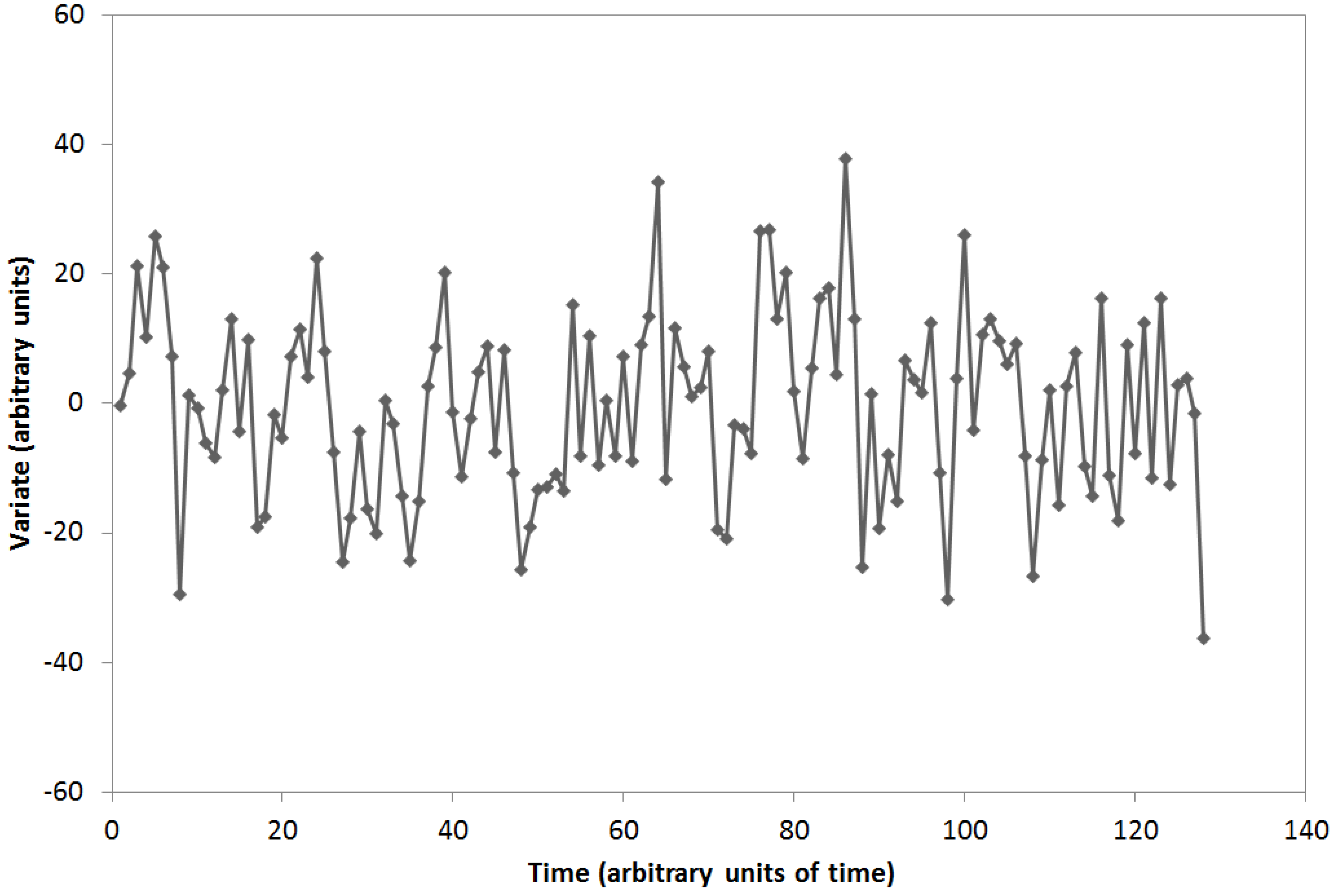
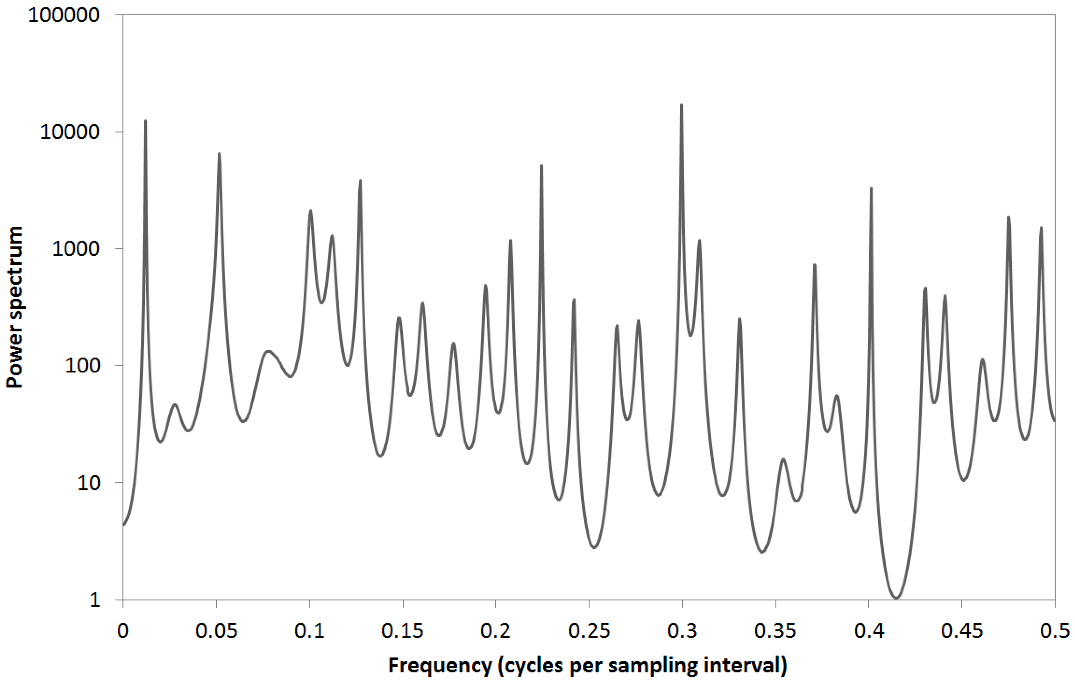
A time series with a constant sampling interval of 1 arbitrary unit of time and arbitrary units of the variable was simulated and is shown in
Figure 1. The number of data is
N = 128, which can be considered a short time series and, thus, a more challenging problem in spectral estimation.
The signal in
Figure 1 consists of the superposition of 11 sinusoids of equal amplitude and the frequencies given in
Table 1. Each sinusoid presented a variance of 10, so the power of the signal was 110. The white noise was generated from a uniform distribution with zero mean and a variance (power) of 75. This simulation is similar to the one used by Vellante and Villante (1984, [
10]) and Pardo-Igúzquiza and Rodríguez-Tovar (2005, [
7]). The time series power spectrum estimated by the maximum entropy method is given in
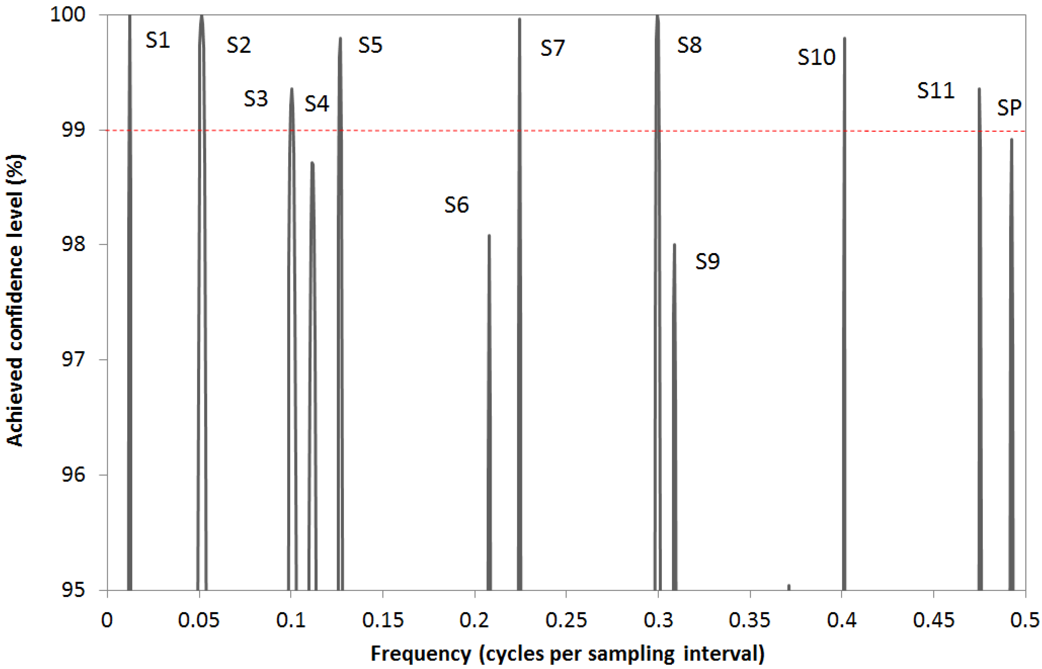
Figure 2. It may be difficult to decide which of the spectral peaks are statistically significant and not spurious. Thus, we calculated the achieved confidence level (ACL) obtained by the permutation test and this is shown in
Figure 3. Taking the 95% ACL, it can be seen in
Figure 3 that the 11 sinusoidal components of the signal were identified (labeled S1 to S11 in
Figure 3). Only one spurious peak (denoted SP in
Figure 3) exceeded the 95% ACL. The high number of spurious peaks in
Figure 2 is the result of using a high AR order (64 terms,
i.e., half the length of the time series) in order to resolve the different components. The spurious frequency in
Figure 3 is very close to the Nyquist frequency, which is a typical result of using a high AR order that is starting to fit thenoise. The maximum entropy estimated frequencies are given in
Table 1. In a practical situation with such a short time series and where the spectral content is generally unknown in advance, only the most significant peaks (ACL above 99.9%) would be considered as a signal (S1, S2, S7, and S8).
Figure 1.
Simulated time series with 128 data and constant sampling interval of one unit. This zero-mean time series is the addition of two components: signal and noise. The variance of the signal is 110 and the variance of the white noise is 75. The spectral content of the signal is given in
Table 1.
Table 1.
Nominal frequencies of the signal, as well as frequencies of the power spectrum estimated by maximum entropy and its achieved confidence level (ACL).
Table 1.
Nominal frequencies of the signal, as well as frequencies of the power spectrum estimated by maximum entropy and its achieved confidence level (ACL).
| Signal | Nominal | Estimated | ACL (%) |
|---|
| S1 | 0.01 | 0.012 | 100 |
| S2 | 0.05 | 0.0515 | 100 |
| S3 | 0.1 | 0.105 | 99.36 |
| S4 | 0.11 | 0.112 | 98.7 |
| S5 | 0.125 | 0.127 | 99.8 |
| S6 | 0.2 | 0.208 | 98.08 |
| S7 | 0.225 | 0.225 | 99.96 |
| S8 | 0.3 | 0.3 | 100 |
| S9 | 0.305 | 0.309 | 98 |
| S10 | 0.4 | 0.402 | 99.8 |
| S11 | 0.475 | 0.475 | 99.36 |
Figure 2.
Power spectrum of the time series shown in
Figure 1, estimated by maximum entropy with an autoregressive model of 64 terms. The Nyquist frequency is 0.5 which corresponds to a period of 2 arbitrary units of time.
Figure 2.
Power spectrum of the time series shown in
Figure 1, estimated by maximum entropy with an autoregressive model of 64 terms. The Nyquist frequency is 0.5 which corresponds to a period of 2 arbitrary units of time.
Figure 3.
Achieved confidence level of the estimated power spectrum shown in
Figure 2. It can be seen that all the spectral peaks have an ACL higher than 95%. There is a spurious peak (SP) in the high frequencies. The Nyquist frequency is 0.5 which corresponds to a period of 2 arbitrary units of time.
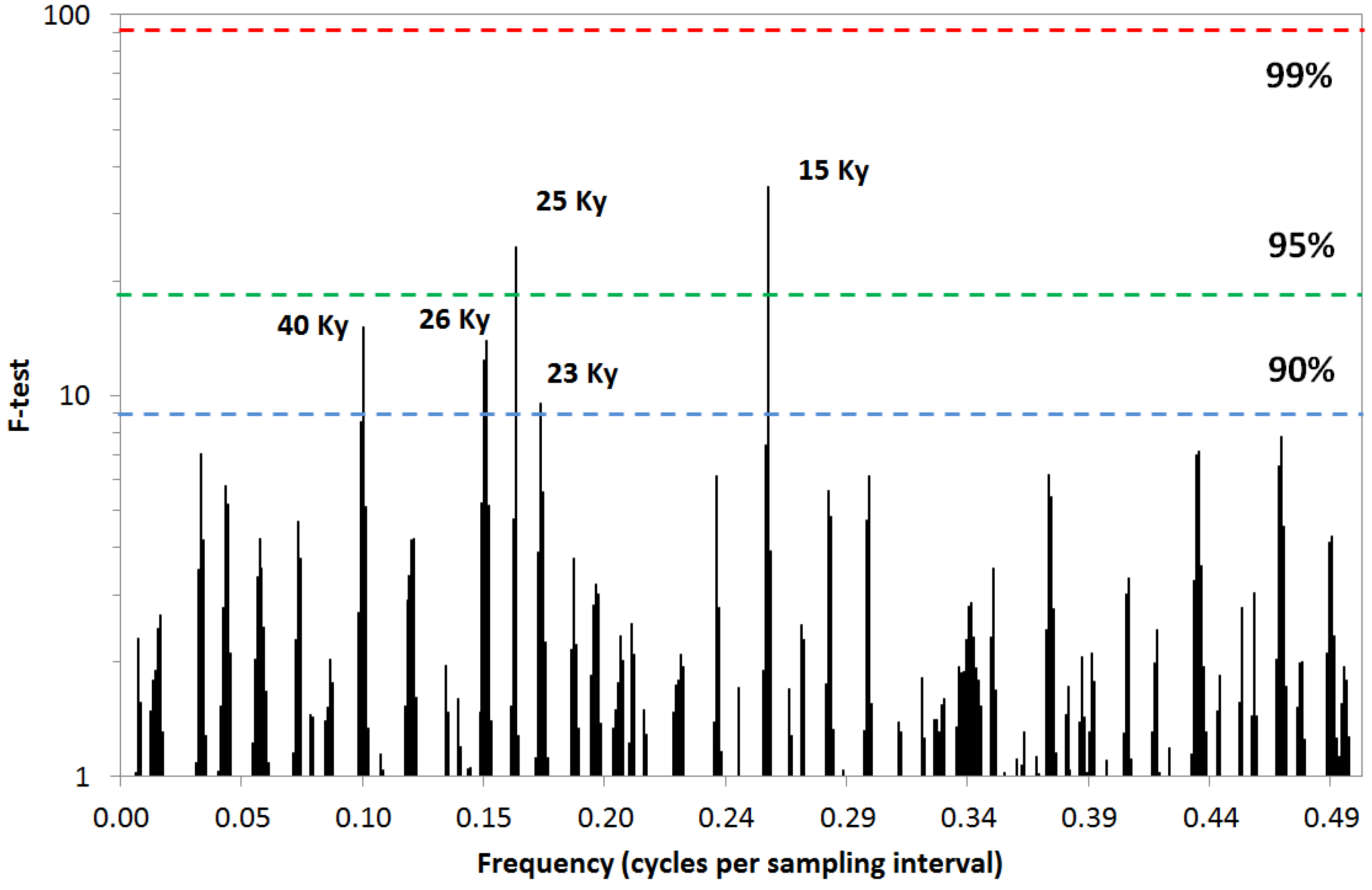
In order to compare the performance of the random permutation test with other parametric estimators, the Thomson multitaper estimator (Thomson, 1982, [
3]; Pardo-Igúzquiza
et al., 1994, [
11]; Lees and Park, 1995, [
9]) with its associated
F-test of statistical confidence was chosen. The tapers used are discrete prolate spheroidal sequences (Thomson, 1982, [
3]). The power spectrum estimated by the multitaper method is shown in
Figure 4. Again, it is difficult to discern which of these peaks are significant. The method was tuned to yield the most favorable estimates when analyzing such a short time series (
Figure 1). Thus, the number of tapers was set at 5 and zero padding was performed, completing up to 1024 data. The results of the
F-test are shown in
Figure 5, together with the 90%, 95% and 99% thresholds in order to interpret the statistical confidence of the results. The first thing that can be seen is that S1, S4 and S5 were not detected with a statistical confidence higher than 90%; Second, there are six clearly spurious (SP) peaks with a statistical significance higher than 90%; Third, the peak with the highest confidence level (>99%) is spurious, and fourth, only two peaks (S3 and S11) were detected with a confidence level higher than 99%. Overall, the results obtained from this advanced parametric test can be considered inferior to those obtained with the random permutation test described above.
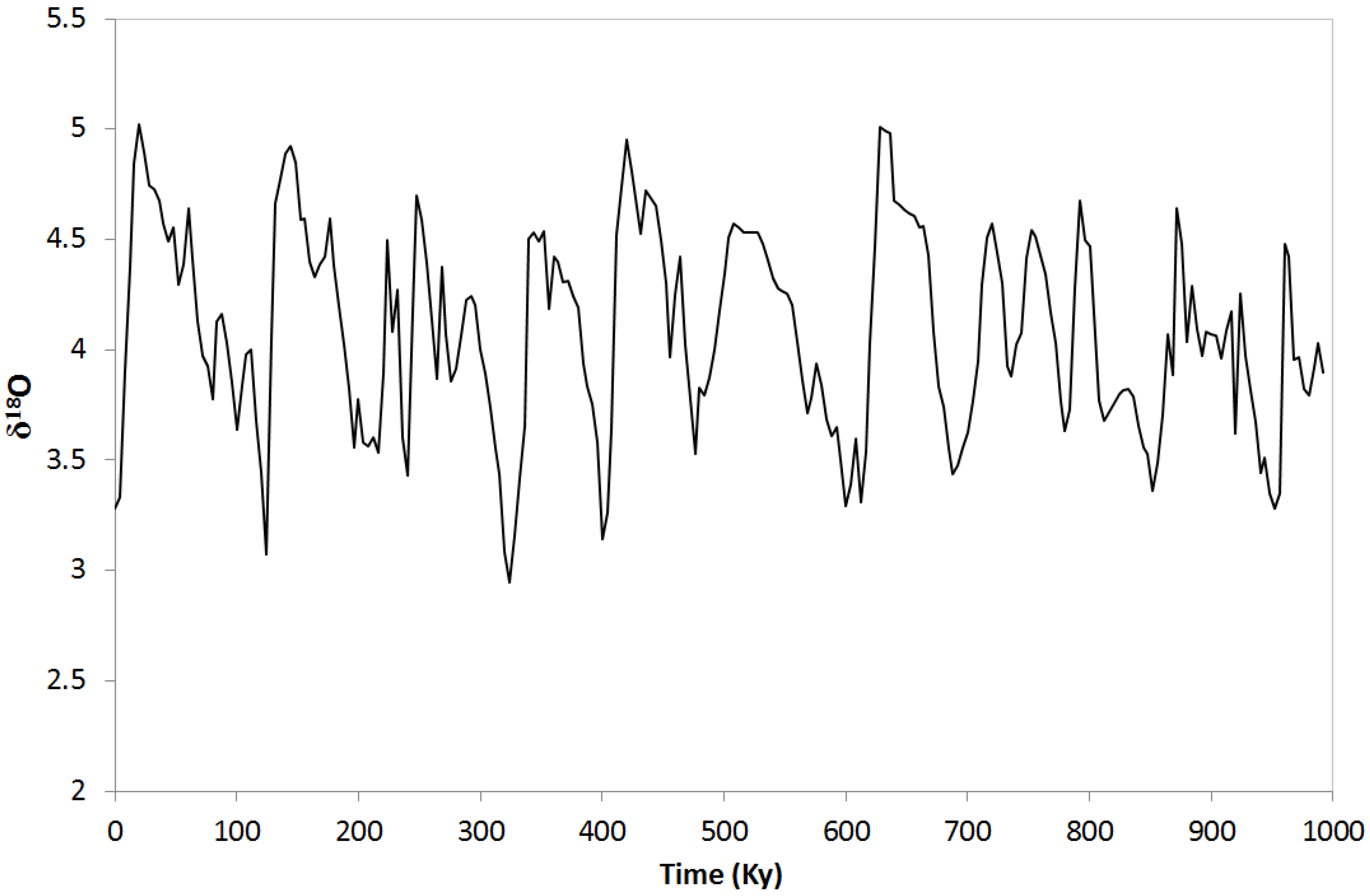
A second case study involved the spectral analysis of a real time series pertaining to a core obtained from site 607 of the Deep Sea Drilling Project (Raymo
et al. 1992, [
12]). The variable is
and a representation of the time series can be found in Park and Maasch (1993, [
13]). The sampling interval is 4 Ky and from the whole time series, a subseries of the last million years was selected. The time series contained 249 data and is shown in
Figure 6. The same methodologies were used as with the synthetic time series.
Figure 7 shows the power spectrum estimated by the maximum entropy method, while
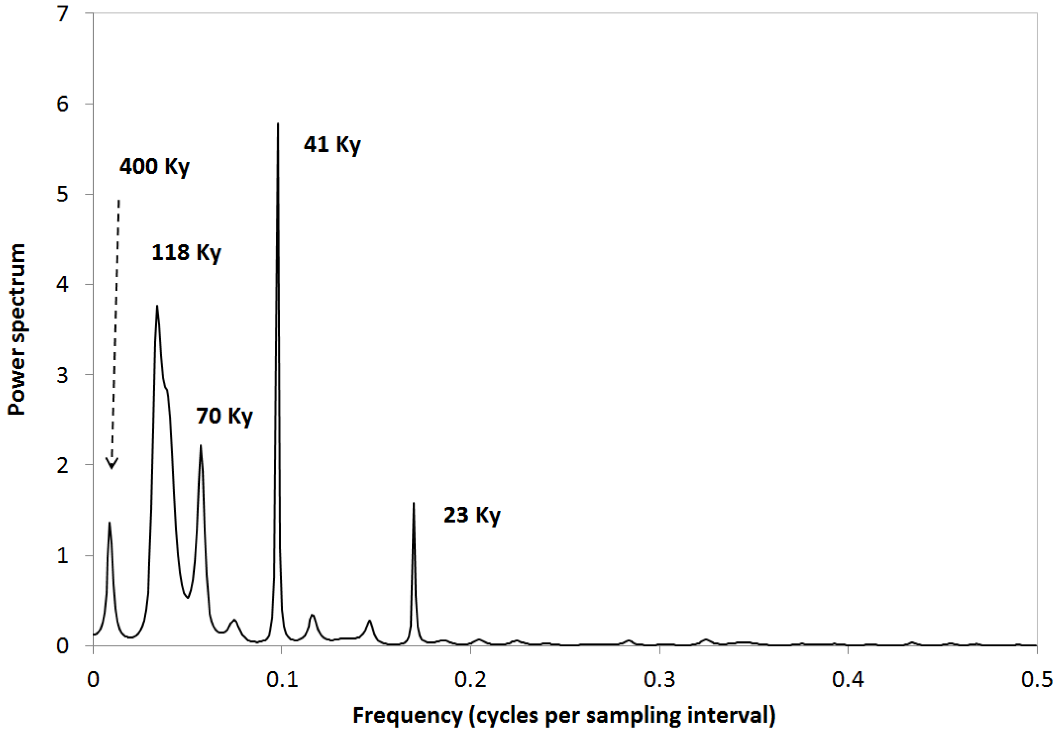
Figure 8 shows the achieved statistical confidence obtained for the permutation test. It can be seen that all the peaks with a confidence level higher than 90% also had a confidence level above 99%. These peaks had periods of 400 Ky, 118 Ky, 70 Ky, 41 Ky and 23 Ky.
Figure 4.
Power spectrum estimated by the Thomson multitaper method with 5 tapers. The Nyquist frequency is 0.5 which corresponds to a period of 2 arbitrary units of time.
Figure 4.
Power spectrum estimated by the Thomson multitaper method with 5 tapers. The Nyquist frequency is 0.5 which corresponds to a period of 2 arbitrary units of time.
Figure 5.
Statistical confidence levels of the power spectrum shown in
Figure 4, calculated by the
F-test associated with the Thomson multitaper estimator. The Nyquist frequency is 0.5 which corresponds to a period of 2 arbitrary units of time.
Figure 5.
Statistical confidence levels of the power spectrum shown in
Figure 4, calculated by the
F-test associated with the Thomson multitaper estimator. The Nyquist frequency is 0.5 which corresponds to a period of 2 arbitrary units of time.
Figure 6.
Real time series of
O of the DSDP607 series with 249 data and a sampling constant interval of 4 kiloyears (Ky).
Figure 6.
Real time series of
O of the DSDP607 series with 249 data and a sampling constant interval of 4 kiloyears (Ky).
Figure 7.
Power spectrum of the time series shown in
Figure 6, estimated by maximum entropy (with 64 autoregressive terms). The Nyquist frequency is 0.5, which corresponds to a period of 8 Ky.
Figure 7.
Power spectrum of the time series shown in
Figure 6, estimated by maximum entropy (with 64 autoregressive terms). The Nyquist frequency is 0.5, which corresponds to a period of 8 Ky.
Figure 8.
Achieved confidence level of the estimated power spectrum shown in
Figure 7. It can be seen that all the spectral peaks have an ACL higher than 99.5%. The Nyquist frequency is 0.5, which corresponds to a period of 8 Ky.
Figure 8.
Achieved confidence level of the estimated power spectrum shown in
Figure 7. It can be seen that all the spectral peaks have an ACL higher than 99.5%. The Nyquist frequency is 0.5, which corresponds to a period of 8 Ky.
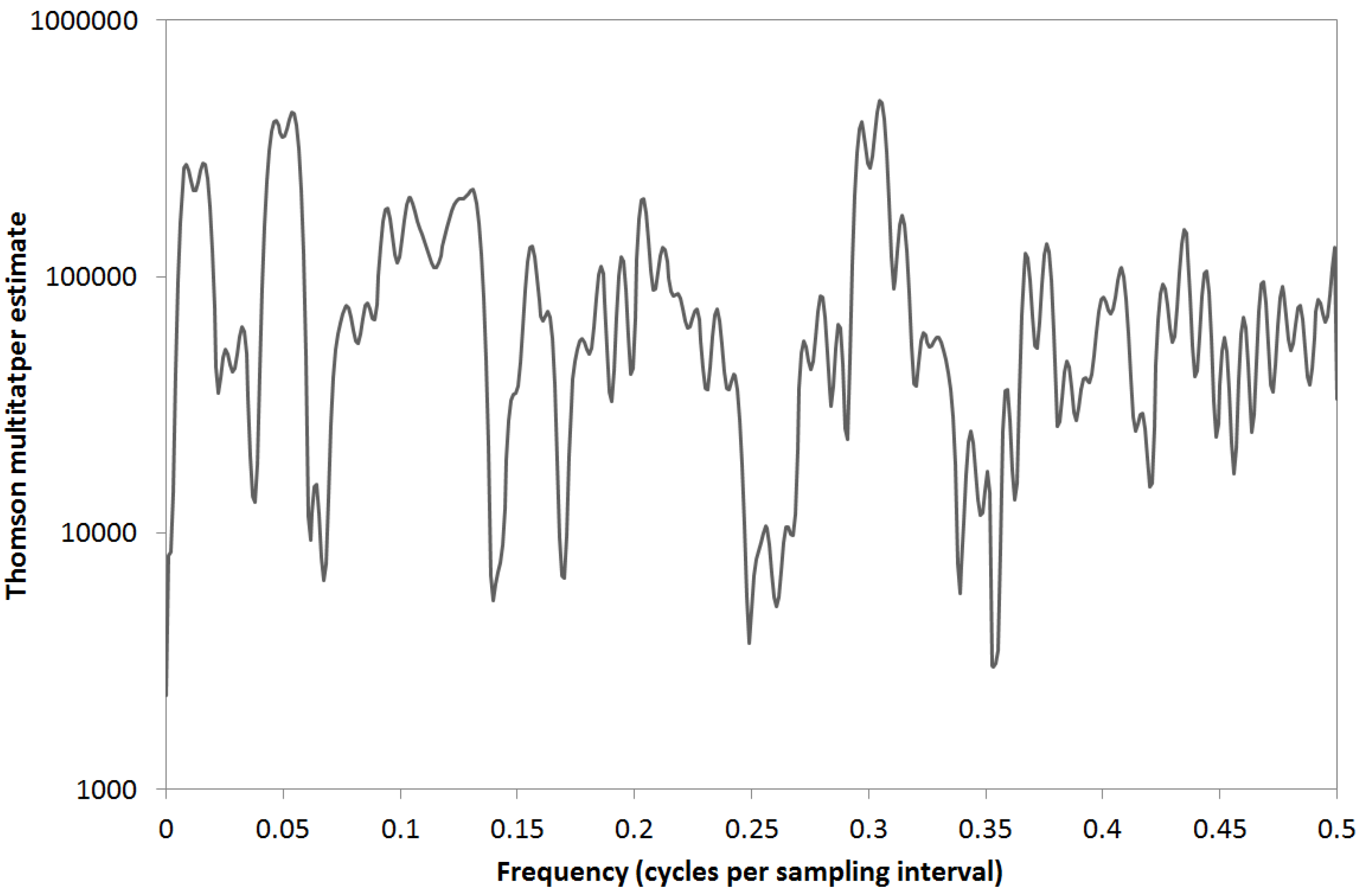
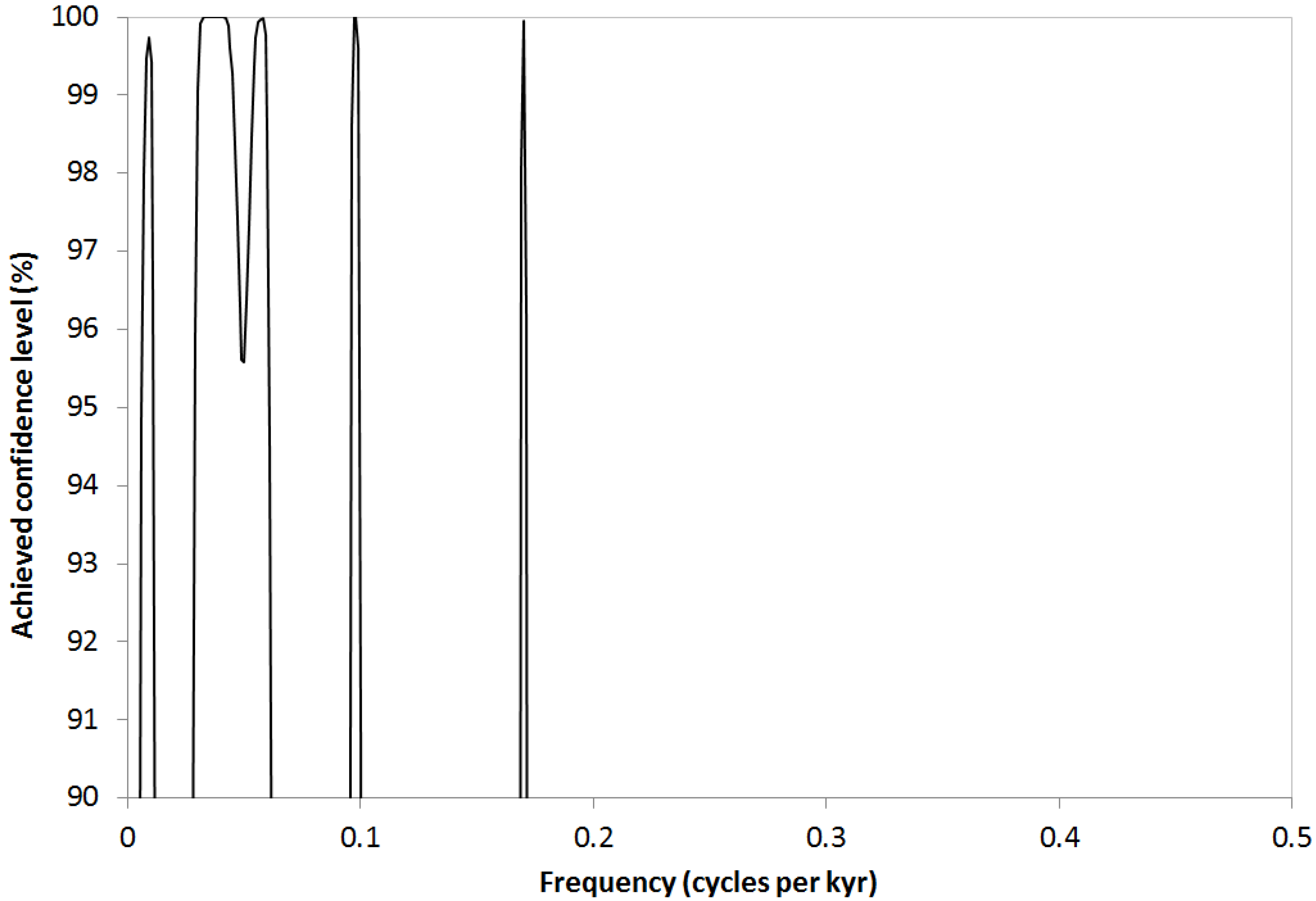
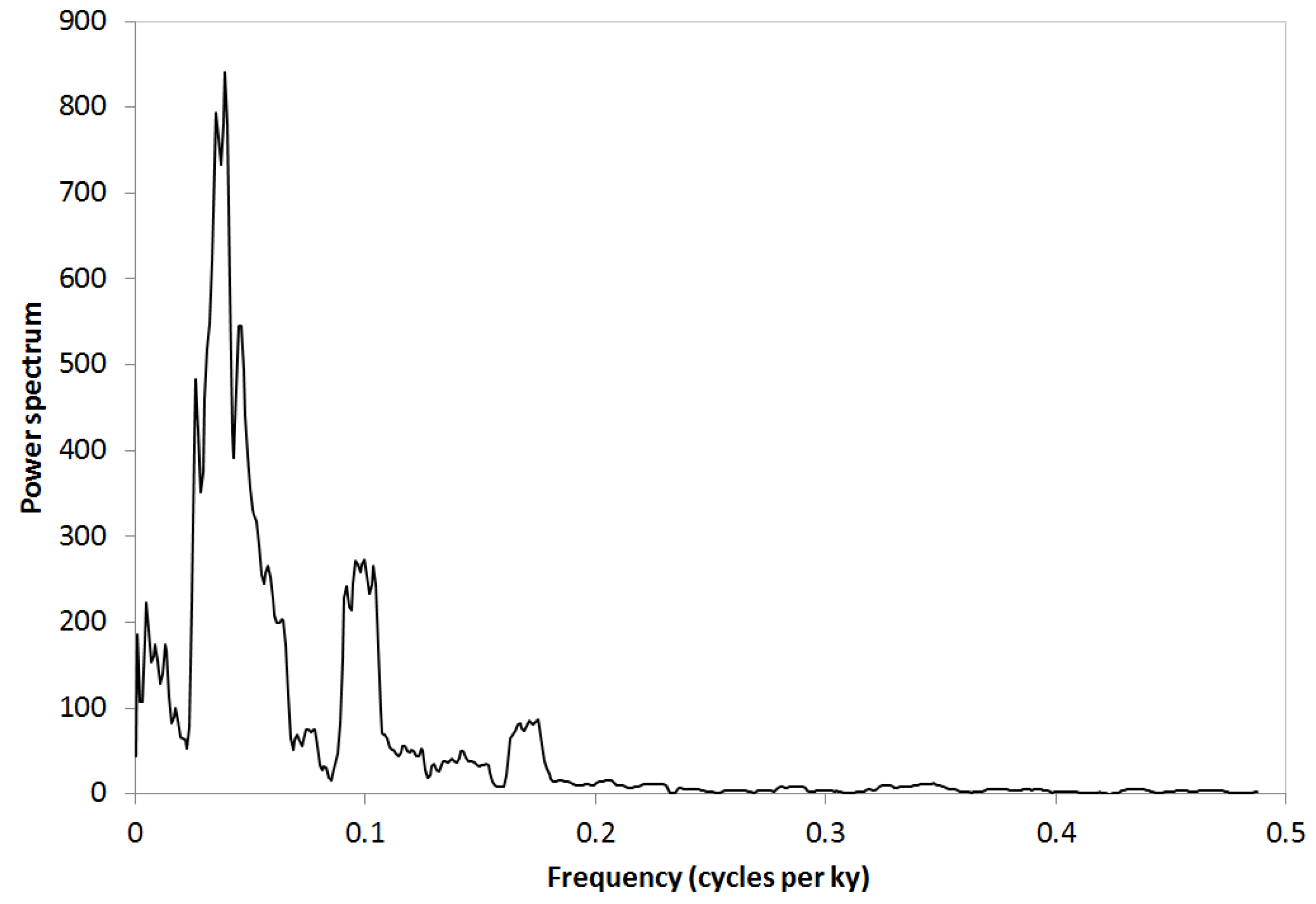
Meanwhile, the power spectrum estimated by the Thomson multitaper method is shown in
Figure 9, and the statistical confidence of the power spectrum as evaluated by the
F-test is given in
Figure 10. The
F-test detects the peaks of 40 Ky, 26 Ky, 25 Ky, 23 Ky and 15 Ky peaks. In the low frequencies the test fails to detect the long and short eccentricity cycles of 400 Ky and 110 Ky. The obliquity cycle is detected but the eccentricity cycle is split in 25 Ky and 23 Ky. Furthermore, the 15 Ky has not been reported as a combination tone between the orbital Milankovitch cycles of eccentricity, obliquity and precession (Wigley, 1976, [
14]), but has been detected as significant by the
F-test. On the other hand the 26 Ky cycle is close to one of those combination tones (Pardo-Igúzquiza and Rodríguez-Tovar, 2000 [
15]).
Figure 9.
Power spectrum estimated by the Thomson multitaper method with 5 tapers. The Nyquist frequency is 0.5, which corresponds to a period of 8 Ky.
Figure 9.
Power spectrum estimated by the Thomson multitaper method with 5 tapers. The Nyquist frequency is 0.5, which corresponds to a period of 8 Ky.
Figure 10.
Statistical confidence levels of the power spectrum shown in
Figure 9, calculated by the
F-test associated with the Thomson multitaper estimator. The Nyquist frequency is 0.5, which corresponds to a period of 8 Ky.
Figure 10.
Statistical confidence levels of the power spectrum shown in
Figure 9, calculated by the
F-test associated with the Thomson multitaper estimator. The Nyquist frequency is 0.5, which corresponds to a period of 8 Ky.
4. Discussion and Conclusions
In modern statistical practice, the reliability or statistical significance of any set of estimates should always be given. This is important in order to arrive at a robust and objective interpretation of the results obtained. In spectral analyses of time series aimed at detecting sinusoidal signals immersed in noise, it is necessary to assess the likelihood that the calculated power spectrum estimates are the result of pure chance. Parametric statistical tests are based on distributional assumptions that are not always met, whereas computer intensive methods dispense with those assumptions but at the expense of more computing time. Now that computer time is no longer a limiting issue, these methods have become more attractive. Here, we have presented the permutation test for assessing the statistical significance of peaks in the power spectrum versus a white noise background. The method is easy to implement and is applicable to any spectral estimator. The method has been shown to yield better results than the F-test associated with the Thomson multitaper spectral estimator. In particular, the F-test seems to miss the low frequency cycles and detect too many significant peaks in the middle range of frequencies. Although only two times series have been used in this work, both time series are general in the sense that there is no a priori advantage for the maximum entropy method (for example, the simulated time series has not been simulated has an autoregressive process). Furthermore, the programs and the data are freely provided by the authors for replicating the results or applying the methods to other time series.
Nevertheless, for the spectral analysis of time series in paleoceanography studies, we would recommend employing the same strategy that has been used for a long time in paleoclimatology (Pestiaux and Berger, 1984, [
16]), namely the use of several spectral methods in order to leverage the advantages of each.


