Abstract
Scour near various offshore structures has been studied by performing numerical model runs with the modified (Fortran) SEDTUBE model, as a follow-up of an earlier paper on scour near marine offshore structures. A fairly simple 1D numerical model (SEDTUBE model) for the computation of sand transport rates and scour depths near structures on the seabed (berms, bed protections) is proposed, tested and validated. The model domain is a stream tube (varying or constant width) including the loose seabed and the hard layers of (multiple) structures. Hence, the model computes the sediment transport along the bed and over the structure(s). The SEDTUBE model can predict the time evolution of free scour depth around rock berms; bed protections; and pile-type structures, as well as the edge scour further away from the pile, in unidirectional and bidirectional tidal flows (weak and strong currents) in combination with waves over a sandy sediment bed with d50 in the range between 0.2 and 2 mm. Five laboratory and four field cases have been used for validation of the model. The model is much more than a scour model; it can also be used for the prediction of sedimentation in shipping channels. The model is valid for sandy beds and for mud–sand beds with slight cohesive properties.
1. Introduction
Structures deployed on a sandy bed (piles, piers, caissons, rock berms, etc.) are sensitive to scour, particularly in the case of fine sand (<0.3 mm) and strong tidal currents in combination with storm waves. Severe scour can endanger the stability of the structure, which can be mitigated by the construction of bed protections around the structure.
Most early scour studies are related to the scour around bridge piers in rivers in conditions with clear-water scour and live-bed scour. Later on, the scour around monopiles in coastal seas was studied extensively, related to the development of offshore wind turbine parks.
Experimental data of free scour development around pile-type structures are abundantly available in the international literature, as discussed by Van Rijn et al., 2025 [1], and in the reviews of Melville (2008) [2] and Liang et al. (2020) [3]. Gong et al., 2025 [4], and Garcia et al., 2025 [5], have given detailed overviews of laboratory and field scour data for offshore wind turbine piles. Furthermore, they have performed new large-scale experiments in a wave-current basin on the scour near piles under irregular waves.
Cui et al., 2025 [6], discussed recent advancements and insights of scour prediction, monitoring and protection measures. Similarly, Yu et al., 2025 [7], and Duan et al., 2025 [8], have given comprehensive reviews of the influencing factors, prediction methods and future directions. As regards prediction methods, they have given informative overviews of various types of numerical models for local scour, including the physical process equations involved. Duan et al., 2025 [8], distinguished (1) CFD-based single-phase models, (2) two-phase flow-sediment models and (3) CFD-SPH flow-sediment models.
CFD models solve the three-dimensional Reynold-averaged Navier–Stokes (RANS) equations for fluid dynamics and can accurately compute the hydrodynamic parameters involved (fluid velocity, pressure and turbulence intensities), which are coupled to sediment transport formulations in an iterative way until reaching the equilibrium state of scouring. A problem is the high computational run time involved, which severely limits the widespread application of these complex models in engineering practice.
Two-phase flow models solve both the fluid dynamics phase as well as the sediment dynamics phase (coupled equations for interaction processes) including initiation, erosion, suspension and settlement of the sediment particles. This method can accurately simulate the overall scour evolution but also reveal the microscopic fluid–particle interactions and inter-particle contacts, offering a powerful tool for studying scour problems in marine engineering. Similarly, the excessive computational time still is a major problem to be solved.
The SPH method (in combination with the CFD flow model) discretizes the computational domain into a swarm of particles carrying physical attributes such as density, mass and velocity for accurate computation of the sediment particle motions and diffusion processes. Advantages of this method are the mesh-free nature and complex boundary handling. However, the large-scale engineering application of this method is problematic for reasons of the extreme computer power involved (requiring parallel computing), which is an order of magnitude greater than that of the traditional grid-based models.
Duan et al., 2025 [8], concluded that numerical scour models are important tools for scour predictions, but their engineering applications still face significant accuracy problems, because mostly laboratory scour data are used for validation, which may be prone to scale errors, particularly for major storm events. Given these problems, there is an urgent need for high-quality field data and technology.
Herein, the development of a more practical scour model for short-term as well as long-term scour predictions is a focus point.
Scour around structures is caused by local fluid accelerations/decelerations and the associated production of extra turbulence. The scouring processes with fluid accelerations, decelerations and vortex generation are rather complex and three-dimensional. As reliable and practical scour models for short- and long-term predictions are missing at the present stage of research, the assessment of the maximum scour depth often requires physical scale modeling. A basic problem of physical scale modeling is that not all parameters can be scaled down with sufficient accuracy. The most problematic parameter is the sediment diameter. Cohesionless sand with a size of 200 μm can be scaled to about 70 μm. Further downscaling to below 70 μm may easily lead to sediment with different (cohesive) properties and thus to scale errors.
Based on the experimental results of scour depth around various types of structures, researchers from Deltares [9,10] and HR Wallingford [11,12,13] have developed a range of empirical scour depth equations. As these types of empirical formulations have no general validity, each equation is only valid for a specific regime, requiring a set of selection criteria to find the proper equation for a certain structure and hydro-dynamic conditions. Furthermore, these empirical models can only predict the maximum scour depth, while the scour pit geometry and the time scale to reach maximum scour depth generally are not included.
Detailed 2DH/3D models, including simulations of increased turbulence levels and sediment entrainment and transport for long-term scour predictions, are still in their infancy [8,14]. Short-term predictions for simple structures are possible, but long-term predictions are not yet feasible. In [1], two scour models were proposed: (1) an empirical scour model (SEDSCOUR) for the prediction of the maximum scour depth without considering the scour hole geometry and (2) a detailed 2DV scour model (SUSTIM) for the prediction of scour hole development over time. However, this latter model cannot represent the additional turbulence generated in the lee zone of the structure and the transport of sediment over a hard-bed protection layer, while the computation time is substantial (hours) for long-term results.
To overcome these problems, a fairly simple 1D numerical model (SEDTUBE) for the computation of sand transport rates and scour depths near structures on the seabed (berms, bed protections) is explained and described in this paper, as a follow-up of an earlier paper [1] on scour near offshore structures. Originally, this model was developed for uni-directional flow and sediment transport as an Excel tool. The upstream structure was represented as a turbulence source without physical dimensions (not included in the computational domain). Recently, the model was extended to tidal flow as a FORTRAN model. The SEDTUBE model of LVRS-Consultancy can predict the time evolution of the free scour depth around rock berms, bed protections and pile-type structures, as well as the edge scour further away from the pile in unidirectional and bidirectional tidal flows (weak and strong currents) in combination with waves over a sandy sediment bed with d50 in the range between 0.2 and 2 mm. The model can represent the flow and sand transport along a stream tube with constant or variable width, including hard layers. The model is fairly universal in the sense that it can also be used for the prediction of sedimentation in shipping channels. The model, which is valid for sandy beds and for mud–sand beds with slight cohesive properties, can be used for long-term computations (10 to 50 years; computation time of minutes). Laboratory and field data have been used for model validation.
2. Scouring Processes
2.1. General
The scouring process depends strongly on the approach velocity, the water depth, the sediment size and gradation, the pile diameter and the pile shape. The scour depth is less for coarser sediments and for sediments with a wider gradation (armoring effects) but the same d50.
Generally, two types of scouring conditions are distinguished [15,16], as follows:
- Clear-water scour: The approach velocity is slightly below the (critical) flow velocity for initiation of motion (ucr); the upstream flow has no sediment load; and scour is initiated by the flow velocity increase around the upstream half of the pile and the extra turbulence and associated vortices generated in the lee zone of the pile.
- Live-bed scour: The approach velocity is higher than the (critical) flow velocity for initiation of motion (ucr); the upstream flow has a sediment load; and the sediment transport capacity around the pile is substantially higher than upstream.
Generally, two scour regions can be distinguished (see Figure 1):
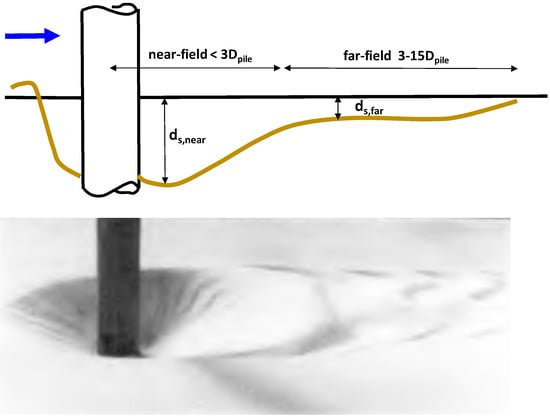
Figure 1.
Near-field and far-field free scour.
- Near-field zone: within a distance of 3 to 5 times the length or height scale of the structure/obstacle from the source location, where a deep scour hole is generated;
- Far-field zone: where a shallow scour hole is generated gradually, reducing to zero further away from the structure; erosion in this zone is often masked by the presence of migrating bed forms (mega-ripples, dune-type forms).
2.2. Berms and Sills
The flow downstream of a two-dimensional sill or other obstacle on the bed is strongly distorted by a recirculation zone and a mixing layer with eddy/vortex generation along the recirculation zone, which is situated between the end of the bed protection and the reattachment point at a distance of about 5 to 7 times the structure height [15]. Usually, the riverbed downstream of a berm, sill or barrage is protected over a certain distance of 10 to 20 times the height of the upstream obstacle/structure to enhance the readjustment of logarithmic velocity profiles and, with that, to reduce the scour of the sediment bed, which strongly depends on the excess (extra) turbulence generated.
Two-dimensional vertical scour downstream of a structure such as a berm, sill or weir in unidirectional river flow has been studied by many researchers (see overview of Hoffmans and Verheij, 1997 [15]; Breusers and Raudkivi [16]). The maximum scour depth in the equilibrium situation as well as the development in time of the scour depth have been studied; see Figure 2.
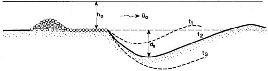
Figure 2.
Two-dimensional scour downstream of structure.
Breusers, 1967 [17], of Deltares studied the time-dependent behavior of scour holes in sandy beds. Based on experimental research in flumes, the time-dependent development of the scour depth in clear water flows was found to be [17]
where ds(t) = maximum scour depth at time t below the original bed (see Figure 2); ho = upstream water depth; and Ts = time (in hours) at which ds = h0.
ds(t)/ho = (t/Ts)0.38
The time evolution to equilibrium conditions in clear-water scour is a gradual asymptotic behavior of the type ds,t = ds,eq [1 − exp(t/Ts)] with Ts = time scale depending on the type of structure, flow velocity, water depth and sediment size. In live-bed scour, the maximum scour depth is more rapidly established, but the equilibrium scour depth may oscillate somewhat due to the passage of migrating bed forms.
The time scale Ts (in hours) was found to be [17,18]
where uo = depth-averaged velocity just upstream (x = 0) of the scour hole; ucr = critical depth-averaged velocity (initiation of motion); ho = upstream water depth; s = specific density (ρs/ρw); ρw = fluid density; ρs = sediment density; and α = coefficient depending on the flow and turbulence structure at the upstream end of the scour hole (α = 1.7 for two-dimensional flow without structure and α = 3 for very violent three-dimensional flow, Van der Meulen and Vinjé, 1975 [19]). The α-coefficient is related to the relative turbulence intensity, ro = σu/u, directly upstream of the scour hole (σu = standard deviation of the local velocity field; u = time-averaged local flow velocity). For hydraulic rough flow, it was found that α = 1.5 + 5ro. The value of ro depends on the type of structure and the length of the bed protection downstream of the structure. If this length is larger than 30ho, additional turbulence produced by the structure has decayed and the ro-value for uniform flow without a structure can be taken, yielding ro = 0.1 to 0.15. Therefore, it may be better to use α = 1.5 + 5(∆ro), with ∆ro being the excess relative turbulence intensity
Ts = 330 (s − 1)1.7 (ho)2/(αuo − ucr)4.3
Generally accepted formulae for the maximum scour depth in the equilibrium situation are not available. A rough estimate can be obtained from Dietz, 1969 [20]; Schoppman, 1972 [21]
where ds,max = maximum scour depth, Ls,max = maximum scour length, hobs = obstacle/structure height or length scale, and α = 1 + 3ro. Equation (3) is only valid for conditions without the supply of sediment from upstream. The maximum scour depth is much lower if there is a supply of sediment from the upstream river section (or from the flood and ebb direction in tidal flow).
ds,max/hobs = (αuo − ucr)/ucr
Ls,max ≅ 10 ds,max
Dietz [20] has found that α = 1 + 3ro with a range of 1.05 to 1.7, depending on the geometry of the obstacle/structure, where ro = relative turbulence intensity. It may be better to use αd = 1 + 3(∆ro), where ∆ro = excess relative turbulence intensity, so that the α-coefficient goes exponentially back to 1 far away from the structure, where the excess turbulence has decayed. Generally, the decay length scale of excess turbulence is on the order of 20 to 30 times the structure height.
Scour data observed near the storm surge barrier in the Eastern Scheldt, The Netherlands, show scour depths on the order of 0.5 to 1 times the local water depth [15]. The observed scour depths are considerably smaller than those predicted by Equation (3), because of the trapping of sediment supplied from upstream. The bottom slope at the upstream end of the scour hole was found to be quite steep (slopes of 1 to 3), which may easily lead to undermining of the bed protection.
2.3. Pile-Type Structures
A pile-type structure blocks the approaching flow, and the flow velocity decreases to zero in front of the pile due to the buildup of a pressure gradient (water surface in front of pile rises slightly). The pressure gradient also generates a surface roller and downflow, impacting the bed in cases of shallow depth. The boundary layer in the near-bed region separates from the pile surface in three dimensions, resulting in the generation of horseshoe-type and spiral-type vortexes, which are carried downstream by the current.
The increase in velocity due to contraction of streamlines around the pile and the production of extra turbulent energy in the lee zone of the pile (vortex shedding) lead to an increase in the entrainment of sediment and local sediment transport capacity, causing severe scour.
The maximum scour depths depend on the size and strength of the vortices around the pile, particularly in strong currents generating vortex streets. In weak currents superimposed by waves, the scour process is more dominated by small-scale vortex shedding from the pile. In shallow water (ho < Dpile), the downflow can directly impact the bed, reducing the generation of horseshoe-type vortices with an opposite direction of rotation and resulting in a smaller scour depth at the same current velocity (ds,max/Dpile = 1.5 to 2) [2,15]. In deep water (ho > 3Dpile), the horseshoe-type and spiral-type vortices near the bed can develop fully depending on the pile dimensions and pile shape, resulting in higher scour depths (ds,max/Dpile = 2 to 2.5) [2,15].
Many experiments on pile scour have been described in the international literature (see review of Liang et al., 2020 [3]). Most experiments are performed using the clear-water scour regime, because the scour pit is significantly larger than in the presence of sediment transport. When sediment is transported, the particles tend to fall into the pit and partially fill it, thereby limiting the scour depth, and the flow’s capacity to scour material from the bed is reduced under these conditions. It is noted that clear-bed scour experiments are far simpler than live-bed scour experiments, which require the recirculation of both water and sediment to generate upstream sediment load in the flow [16].
Scour patterns observed in field conditions with tidal currents superimposed by waves are rather scarce. More field measurements on this should be performed.
3. Description of SEDTUBE Scour Model
3.1. General
The SEDTUBE1D model is a one-dimensional FORTRAN model for the simulation of the morphological evolution of the underwater bed under the influence of (tidal) currents and waves (Van Rijn 2005, 2017 [22]) including the effect of structures generating extra turbulence; see Figure 3. This type of structure-related turbulence is extra turbulence in addition to the normal turbulence generated within the boundary layer, which does not increase further once generated. Normal turbulence is automatically included in the SEDTUBE model through the bed shear stress and fluid mixing parameters, resulting in suspended load transport. Often, this is the primary cause of scouring processes, particularly in clear-water scour.
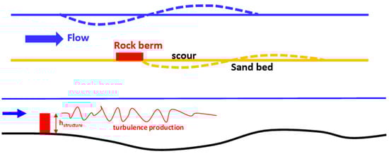
Figure 3.
Scour downstream of rock berm.
The model computes the bed load and suspended load transport, including the effects of wave-induced stirring of sediments. The adjustment of the suspended sediment concentration is simulated by an exponential adjustment equation. The adjustment factor of this latter equation is represented by a parameterized function, which is based on computed results of a more advanced two-dimensional–vertical morphological model (SUTRENCH-model; Deltares, 1985 [23], Van Rijn, 1986 [24]).
3.2. Model Equations
3.2.1. Tidal Flow
Assuming uniform flow conditions in the lateral direction (2D flow), the depth-averaged flow field can be represented as follows:
where, hx = total water depth at time t (m); hMSL = water depth to mean sea level (MSL); hstorm = storm setup (m); bx = width of stream tube; η1,max = amplitude of tidal water level elevation of M1 tide (m); η2,max = amplitude of tidal water level elevation of S1 tide (m); ω1 = 2π/T1 = tidal frequency (1/s); ω2 = 2π/T2 = tidal frequency (1/s); T1 = tidal period of M1 tide (12 h); T2 = tidal period of S1 tide (=12.4 h); Q = tidal discharge at time t (m3/s); ux = depth-averaged flow velocity at time t (m/s); u1,max = peak depth-averaged flow velocity of M1 tide; u2,max = peak depth-averaged flow velocity of S1 tide; and φ = phase difference between horizontal and vertical M1 tide (hours), where positive value means that maximum flood velocity occurs before HW.
Tidal variation: hx = hMSL + hstorm + η1,max sin(ω1t) + η2,max sin(ω2t)
Flow velocity at x = 0: uo,t = Q/(bo ho) = umo + u1,maxo sin(ω1t + φ) + u2,max,o sin(ω2t)
Discharge at x = 0: Q = bo ho uo
Flow velocity at x: ux = Q/(bxhx)
The neap–spring tidal cycle can be included by input values (η2,max ≅ 0.2 to 0.3 η1,max; u2,max ≅ 0.2 to 0.3 u1,max). The tidal period of the S1 tidal cycle (moon cycle) is 12.4 h [25].
The tidal depth-averaged current velocity and the water level variation are described by Equations (1) and (2), where φ = phase angle to account for phase difference between the vertical and horizontal M1 tide. Generally, the peak of the flood current is 2 to 3 h earlier than HW, mostly due to bottom friction effects.
Figure 4 shows the variations in the water level and depth-averaged current velocity for φ = 90° and 180°, where φ = 0° for maximum flood velocity at high water (HW); φ = 60° for maximum flood velocity at 2 h before HW; φ = 90° for maximum flood velocity at 3 h before HW, and φ = 180° for maximum ebb velocity at high tide.
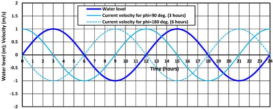
Figure 4.
Phase shift between horizontal and vertical tide (phase shift of 1 h = 30°). η = ηmax sin(ωt) and v = vmax sin(ωt + φ), where ηmax = 1 m, vmax =1 m/s, ω = 2π/T, and T = 12 h.
It is easiest to have flood velocity in the positive x-direction. Generally, the phase angle φ is about 60° (2 h) under field conditions.
An arbitrary stream tube can be defined by specifying the width and water depth along the stream tube (x-direction) as input data. By prescribing the widths and water depths along the tube (Figure 5), the depth-averaged velocity can be prescribed (manipulated), as the discharge in the stream tube is constant, resulting in ux = (Q/bx hx).
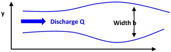
Figure 5.
Arbitrary stream tube with varying width and water depth.
The width data can be obtained from a detailed mathematical model, using laboratory or field measurements.
3.2.2. Effective Flow Velocity for Sediment Transport
The effective flow velocity is defined as ue,x = (1 + rx)ux + 0.4 γe uw,x
Turbulence parameter is schematized, as:
where ro = initial excess turbulence parameter (range 0.2–1); xr = x-coordinate of turbulence source; L1 = 5 γbh1 dobst and L2 = 40 γbh2 dobst; dobs = length scale of turbulence source (m); and γbh1, γbh2 = calibration coefficients (default = 1).
rx = 1 + ro[(x − xr)/(L1)] for xr < x < xr + L1
rx = 1 + ro [1 − {x − (xr + L1)}/(L2)]1.2 for xr + L1 < x < xr + L1 + L2
rx = 1 for x > xr + L2
It is assumed that the extra turbulence increases linearly from 0 to ro over a distance of L1 and that the extra turbulence decays to 0 over a distance of L2. Figure 6 shows the distribution of the r-parameter along the x-axis. The value of the turbulence parameter r increases from r = 1 to r = 1 + ro over distance L1 and decreases to 1 over distance L2.
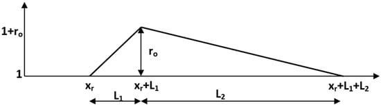
Figure 6.
Distribution of r-parameter along x-axis.
The extra turbulence is only generated downstream of the structure. In the case of tidal flow, scour holes are generated on both sides of the structure. The turbulence parameter causing scour is only applied in the downstream direction. Deposition may take place in the upstream section, where the flow passes the scour hole without extra turbulence.
It is realized that the representation of the structure-related turbulence as a local increase in the depth-averaged velocity (effective velocity) is a practical engineering approach to model the effect of increased turbulence in addition to normal turbulence. In reality, the increased velocity fluctuations produce a non-zero vertical momentum component (due to a change in turbulence or in bed roughness) that increases the bed shear stress, ultimately enabling sediment entrainment.
3.2.3. Sediment Transport
The sediment transport in the stream tube is described as
where Qtotal = total sediment transport (kg/s); Qs = bxqs,x = suspended load transport (kg/s); and Qb = bxqb,e,x = equilibrium bed load transport (kg/s).
Qtotal,x = Qs,x + Qb,x
The suspended load transport is described by
where Qs,x = Q cx = suspended load transport in stream tube (kg/s); c = depth-averaged sediment concentration; ceq = depth-averaged equilibrium sediment concentration; Q = fluid discharge in stream tube (constant); Qs,x,eq = bx qs,e,x = equilibrium sediment transport in stream tube (kg/s); γA = adjustment coefficient (-); and hx = total water depth.
dQs,x/dx = −γA (Qs,x − Qs,x,eq)/hx
Equation (11) describes the adjustment of the depth-averaged sand concentration and the suspended sand transport (Qs = c Q) in a stream tube to the equilibrium values.
Using an upwind scheme, Equation (11) can be approximated by
where K = (γA/hx)∆x = coefficient (-); hx = total water depth; and ∆x = grid size.
Qs,x = Qs,x − ∆x + ∆Qs
Qs,x = Qs,x − ∆x + [(−γA/hx)(Qs,x − Qs,x,eq) ∆x]
Qs,x = Qs,x − ∆x + [−K(Qs,x − Qs,x,eq)]
Qs,x = [Qs,x − ∆x + K Qs,x,eq]/(1 + K)
If γA or K approaches infinity, it follows that Qs,x ≅ Qs,x,eq.
If γA or K approaches zero, Qs,x ≅ Qs,x − ∆x.
The adjustment factor (γA) has been determined by Eysink–Vermaas (1983) [26] from computed results for a wide range of conditions using a detailed suspended transport model [23]. The adjustment factor used herein is a slightly modified version of the adjustment parameter of [26] and reads as
where h = flow depth; ws = fall velocity of suspended sediment; u* = bed shear velocity due to currents and waves (=ueff g0.5/C); C = 5.75 g0.5 log(12hx/ks) = Chézy coefficient; ks = effective bed roughness height of Nikuradse [25]; g = 9.81 = gravity acceleration (m/s2); and αA = coefficient (range 0.1–0.3; higher value gives more rapid adjustment).
γA = αA(ws/u*,x)(1 + 2ws/u*,x)(1 + Hs/htotal,x)2
The adjustment of the suspended transport proceeds relatively rapidly in the presence of waves (see effect of Hs/h parameter). Larger γA-values (larger fall velocity, smaller bed shear velocity, larger relative wave height) lead to more rapid adjustment to equilibrium conditions.
The equilibrium sand transport rates are represented by simple engineering formulations related to the bulk flow parameters (depth-averaged flow velocity, wave height), which can be adjusted by calibration coefficients.
The simplified bed load–load transport formula for steady flow (with or without waves) reads as follows (Van Rijn, 2007 [27]):
where
Qb,e = αb 0.015 (1 − pfines/100) ρs U b h (d50/h)1.2 Me1.5
Qb,e = bed load transport (kg/s);
αb = calibration coefficient (default = 1);
pfines = percentage (%) of fines < 63 µm;
Me = (ue − ucr)/[(s − 1)gd50]0.5 = mobility parameter (-);
ue = ux (1 + rx) + 0.4 γe Uw = effective velocity (m/s);
γe = calibration coefficient (1 for irregular waves and 2 for regular waves);
u = depth-averaged flow velocity (m/s);
Uw = peak orbital velocity (m/s) based on linear wave theory;
Hs = significant wave height (m); Tp = peak wave period (s);
ucr = βucr,c + (1 − β)ucr,w = critical velocity (m/s) with β = u/(u + Uw);
ucr,c = critical velocity (m/s) for currents based on Shields (Van Rijn, 1993 [28]);
ucr,w = critical velocity (m/s) for waves (see Van Rijn, 1993 [28]);
ucr,c = 0.19 (1 + pfines/100)1.5 (d50)0.1log(12h/3d90) for 0.0001 < d50 < 0.0005 m;
ucr,c = 8.50 (1 + pfines/100)1.5 (d50)0.6log(12h/3d90) for 0.0005 < d50 < 0.002 m;
ucr,w = 0.24 (1 + pfines/100)1.5 [(s − 1)g]0.66 d500.33 (Tp)0.33 for 0.0001 < d50 < 0.0005 m;
ucr,w = 0.95 (1 + pfines/100)1.5 [(s − 1)g]0.57 d500.43 (Tp)0.14 for 0.0005 < d50 < 0.002 m.
The suspended load transport for steady flow reads as follows (Van Rijn, 2007 [29]):
where
Qs,e = αs 0.012 (1 − pfines/100) ρs U d50 Me2.4 (D*)−0.6
Qs,e = suspended load transport (kg/s);
h = water depth (m);
d50 = particle size (m);
D* = d50[(s − 1)g/ν2]1/3 = dimensionless particle size (m);
αs = calibration coefficient (default = 1);
s = ρs/ρw = relative density (-);
ν = kinematic viscosity (m2/s);
Me = (ue − ucr)/[(s − 1)gd50]0.5 = mobility parameter;
ue = effective velocity (see Equation (8));
ucr = critical depth-averaged velocity for initiation of motion.
3.2.4. Bed Level Changes
The bed level changes are described by
where zb = bed level to datum; bx = width of stream tube; Qtotal,x = Qb,e + Qs = total load transport (kg/s); ε = porosity of bed material deposits; ρs = sediment density; and γsmooth = smoothing coefficient (range 0.001–0.01).
bx ∆zb/∆t + [(1 − ε)ρs]−1 [∆Qtotal,x/∆x] = 0
∆zb,i,t+∆t = −∆t[{Qtotal,i+1,t − Qtotal,i−1,t} +
0.5 γsmooth(zb,i+1,t − 2zb,i,t + zb,i−1,t)]/[2 bi ∆x(1 − ε)ρs]
0.5 γsmooth(zb,i+1,t − 2zb,i,t + zb,i−1,t)]/[2 bi ∆x(1 − ε)ρs]
The bed level change ∆zb,i,t+∆t is negative (erosion) if the sediment transport increases in the positive x-direction.
As regards the sand transport process on the hard layer (of the structure and the bed protection), three cases can occur:
- No sand is present on the hard layer: sand transport along the hard layer is constant (Qs,i+1 = Qs,i and Qb,e,I = Qb,i−1);
- Sufficient sand is present on the hard layer: the erosion is computed by Equations (12)–(15);
- Insufficient sand is present on the hard layer or the potential erosion thickness (∆zb) is larger than the sand layer thickness (∆zhard): the sand transport is adjusted; see Equation (16).
Qs,i = Qs,i−1 + (∆zhard/∆zb) (Qs,i − Qs,i−1)
Qb,e,i = Qb,i−1 + (∆zhard/∆zb) (Qb,e,i − Qb,e,i−1)
3.2.5. Input and Output Parameters
The input data are
- Water depth values and hard-layer values of bed profile (m);
- Stream tube width values (m);
- x-coordinate values of bed profile (m);
- Grid size values (variable) along domain (m);
- Storm setup above mean sea level (m);
- Tidal amplitude η1,max (m) of M1 tide and η2,max (m) of S1 tide mean flow velocity umo (m/s);
- Maximum (peak) tidal flow velocity u1,max (m/s) of M1 tide and u2,max (m/s) of S1 tide;
- Phase lag φ (hours);
- Tidal period Ttide1 (hours) of M1 tide and Ttide2 of S1 tide;
- Significant wave height Hs (m) and period Tp (s) and duration (days) of each wave condition;
- Water temperature (Celsius); ρw, density of seawater (kg/m3); and ρs, density of sediment (kg/m3);
- Porosity of bed material (-); sand d50, d90 (m);
- ws, settling velocity of suspended sediment for sand (m/s);
- ucr, critical depth-averaged velocity (m/s);
- pfines, percentage fines < 63 µm (%);
- ks, bed roughness (m);
- γbed, (gamb) calibration parameter bed load transport, default (-);
- γsus, (gams) calibration parameter suspended load transport, default = 1 (-);
- γeff, (game) calibration factor effective velocity of waves, default = 1 (-);
- γbh, (gambh) calibration factor for turbulence adjustment distance, default = 1 (-);
- αad, (alfad) coefficient of suspended load adjustment factor, range 0.1–0.3 (-);
- ro, turbulence coefficient (-);
- xr, position from where turbulence coefficient is active (m);
- bh, length scale (width or height) of upstream obstacle/strucure on bed (m);
- ∆t, time step (s);
- γsmooth, (gamsb) bed smoothing factor (-);
- iswr, switch (0/1) equilibrium transport zero transport at boundaries (-);
- resfle, output selection parameters.
Typical grid sizes are 0.05 to 0.2 m for laboratory cases and 0.2 to 2 m for field cases.
Typical time steps are 1 to 10 s for laboratory cases and 10 to 300 s for field cases.
4. Validation of SEDTUBE Model
4.1. General
The following validation cases are presented:
- Laboratory cases:
- -
- Scour downstream of bed protection (no upstream structure);
- -
- Scour downstream of rock berm and bed protection.
- Field cases:
- -
- Scour downstream of culvert in the Eastern Scheldt (NL);
- -
- Scour downstream of rock berm structure, Morecambe Bay, UK;
- -
- Sedimentation in trial dredge trench in the Western Scheldt estuary, NL.
The latter case refers to the sedimentation in a trench to show that the SEDTUBE model is much more than a scour model. It is a universal model in the sense that it can also be used for sedimentation predictions. However, more validation work for typical sedimentation cases is required. It is noted that most of the scour validation cases are from the period before 2020. More recent field validation cases are not yet available. Additional validation work using recent data will be performed later in future research.
4.2. Laboratory Case—Scour Downstream of Bed Protection (No Upstream Structure)
Hoffmans (1990) [30] studied the scour of a sand bed (with a length of about 10 m; thickness = 0.25 m) downstream of a horizontal bed protection of gravel in a laboratory flume (width = 0.8 m) with water flow. The approaching flow was free of sand (no initial sediment load). The bed protection of gravel was horizontal over a length of 10 m without any structure. The development of the scour hole (Test C60) was measured over nearly 30 h; see Figure 7. The basic data of Test C60 are given in Table 1.
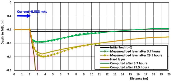
Figure 7.
Measured and computed bed levels of scour hole, Test C60.

Table 1.
Basic SEDTUBE model input parameters; scour downstream of flat bed with bed protection (Test C60).
The SEDTUBE 1D model has been used to simulate the scour downstream of the bed protection. This model computes the depth-averaged flow velocity and suspended plus bed load transport in a stream tube. The gradual adjustment of the suspended sand transport to the local flow conditions is represented by an empirical function. The bed load transport and the suspended sand transport at x = 0 are set to zero (no initial load).
The effect of additional turbulence in the downstream deceleration zone is taken into account by the r-parameter acting on the mean current velocity ue = (1 + r)u.
Figure 7 shows the measured and computed bed levels of the scour hole in the sand bed (x > 0) downstream of the bed protection for Test C60. The parameters of the r-distribution are ro = 0.3; L1 = 1.6 m; and L2 = 16 m. The agreement between the measured and computed values is quite good after 3.7 h. The computed bed levels after 29.5 h are slightly too low (underprediction). The model tends to underestimate the depth of scour as time passes.
4.3. Laboratory Case—Scour Downstream of Rock Berm and Bed Protection
Many scour tests have been performed in various flumes by Deltares (Report M648-863, 1972) [31] in the period from 1960 to 1970. Herein, the scour results of Test S11-12B and Test S20-3 have been used for calibration of the SEDTUBE model. These tests refer to the basic case of clear water scour (no upstream transport) downstream of a rock berm, as discussed in Section 2.2. The sand bed downstream of the berm and bed protection consisted of fine sand with d50 = 0.12 mm. The critical depth-averaged flow velocity causing initiation of movement of sand particles was found to be 0.26 m/s (computed value = 0.28 m/s) for Test S11-12B and 0.38 m/s (computed 0.33 m/s) for Test S20-3. The basic input data are given in Table 2.
Table 2.
Basic SEDTUBE model input parameters; scour downstream of rock berm for Test S11-12B and TestS20-3.
Figure 8 and Figure 9 show the measured and computed scour bed levels in Test S11-12B and Test S20-3. The computed maximum scour depth is somewhat too large (conservative prediction). Hence, the model tends to overestimate the depth of scour slightly.
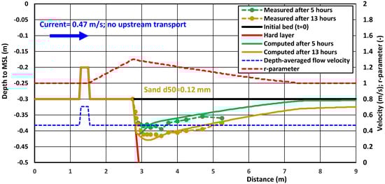
Figure 8.
Measured and computed bed levels of scour hole, Test S11-12B.
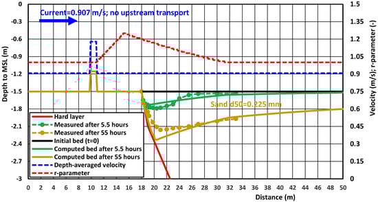
Figure 9.
Measured and computed bed levels of scour hole, Test S20-3.
4.4. Laboratory Case—Scour Around Piles in Uni-Directional Flow
Sheppard and Miller (2006) [32] measured the scour depth around a monopile in a laboratory flume with a sand bed (d50 = 0.27 mm; ucr = 0.27 m/s; porosity = 0.4; sediment density = 2650 kg/m3). The water depth was about 0.42 m. The pile diameter was 0.152 m. The approach current velocity was varied in the range of 0.17 to 1.64 m/s; see Table 3.
Table 3.
Measured and computed scour depth and model coefficients; Sheppard-Miller test 2006 [32] with water depth = 0.42 m.
The test with a velocity of 0.17 m/s is a clear-water scour test (no sediment load in upstream current); the other tests are live-bed scour tests with recirculation of the sediment load.
The increase and decrease in the depth-averaged velocity along the pile are simulated by narrowing and widening the stream tube; see Figure 10. The upstream width of the stream tube is set to b = 1 m. The depth-averaged velocity increases and decreases from 0.62 m/s to 0.93 m/s and back to 0.62 m/s (factor 1.5 higher [1]) for Test 2. The depth-averaged flow velocity ue = (1 + r)u is also shown. This scheme is applied in all computations. The turbulence parameter (ro) is in the range of 0.3 to 0.7; see Table 3. The basic data and model input coefficients are given in Table 3. The depth-averaged flow velocity represents the flow velocity derived from the discharge measurements. The flow velocity in the center line of the flume is somewhat higher (about 10%).
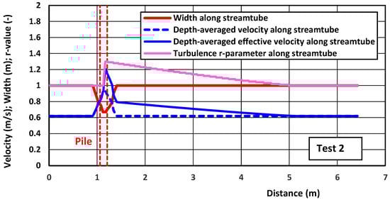
Figure 10.
Width, depth-averaged flow velocity, depth-averaged effective velocity, and turbulence r-parameter along stream tube (Test 2).
The fluid and sediment density are 1000 and 2650 kg/m3. The settling velocity is set to ws = 0.022 m/s. The bed porosity is set to 0.4. The bed roughness is set to 0.01 m. The grid size is 0.01 m. The time step is 0.5 s. The bed smoothing coefficient is 0.01. Equilibrium sediment transport is prescribed at the inlet boundary x = 0 m for Tests 2 to 6. The runtime for 24 h is 6 s. Test 1 is simulated with uo = 0.19 m/s (flow velocity along the axis of the flume is assumed to be higher than 0.17 m/s (based on discharge)) and ucr = 0.2 m/s, resulting in a maximum scour depth of about 0.1 m (measured at 0.13 m).
Figure 10, Figure 11, Figure 12 and Figure 13 show the computed scour profiles near the pile for Tests 2, 5A, and 6. Measured bed profiles were not given by [31]. The time to reach equilibrium scour conditions is about 5 h for Test 2 and less than 1 h for Tests 5A and 6. The maximum scour depth occurs at the downstream side of the pile. The scour extends over a distance of about 4 m (25 pile diameters).
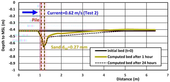
Figure 11.
Computed bed profiles for Test 2.
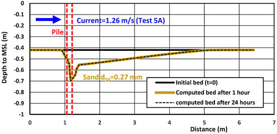
Figure 12.
Computed bed profiles for Test 5A.
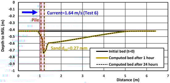
Figure 13.
Computed bed profiles for Test 6.
Figure 14 shows a comparison of the computed and measured maximum dimensionless scour depths (ds,max/Dpile). The horizontal axis refers to the ratio of the current velocity and critical velocity for initiation of motion (u/ucr). The computed values show rather good agreement (about 10% to 15% too high), with measured values for all live-bed scour test results, but the computed value is somewhat too small (15%) for the clear-water scour test result, with relatively low velocity (<0.2 m/s). The computed time scale is 30 h for the clear-water scour tests and less than 1 h for most of the live-bed scour tests. Overall, the model tends to underestimate the clear-water scour and overestimate the live-bed scour slightly.
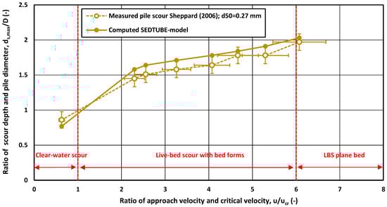
Figure 14.
Computed and measured maximum scour depth for all tests.
Sheppard (2003) [33] measured the scour around a monopile (diameter = 0.305 m) in a long, wide flume with a water depth of 1.22 m above a sand bed with d50 = 0.22 mm, critical velocity ucr ≅ 0.3 m/s, bed porosity = 0.4, and sediment density = 2650 kg/m3. The current velocity was 0.31 m/s. The basic data and model input coefficients are given in Table 4.
Table 4.
Measured and computed scour depth and model coefficients; Sheppard test (2003) [33] with water depth = 1.22 m.
The velocity increase along the pile structure is assumed to be 1.5 [1]. The velocity increase and decrease along the pile are simulated by narrowing and widening the stream tube; see Figure 15. The upstream width of the stream tube is set to b = 1 m. The depth-averaged velocity increases and decreases from 0.31 m/s to 0.46 m/s and back to 0.31 m/s (factor 1.5). The depth-averaged flow velocity ue = 1 + r)u is also shown. The turbulence coefficient is set to ro = 0.2. The fluid and sediment density are 1000 and 2650 kg/m3. The settling velocity is set to ws = 0.02 m/s. The bed porosity is set to 0.4. The bed roughness is set to 0.03 m. The grid size is 0.01 m. The time step is 3 s. The bed smoothing coefficient is 0.01. The sediment transport at the upstream boundary is set to 0 (no transport). The runtime for 200 h is 7 s.
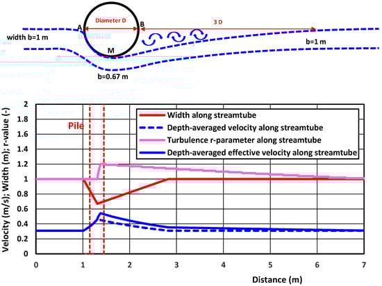
Figure 15.
Width, depth-averaged effective flow velocity, depth-averaged velocity, and turbulence r-parameter along stream tube.
Figure 16 shows the computed scour profiles after 24, 72, and 192 h. The time to reach equilibrium scour conditions is about 200 h. The scour extends over a relatively short distance of about 2 m (6 pile diameters), which is caused by the relatively low flow velocity of 0.31 m/s, just above the critical velocity (about 0.3 m/s).
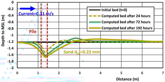
Figure 16.
Computed bed profiles after 24, 72, and 192 h; Sheppard test (2003) [33].
Figure 17 shows the measured and computed maximum scour depth as function of time. The computed maximum equilibrium scour depth is about 0.45 m, which is somewhat higher (20%) than the measured values of 0.37 m (≅1.2 Dpile). The time scale of the measured equilibrium scour depth is about 150 h, which is somewhat shorter than that of the computed value of 200 h. Most likely, the strong effect of the near-bed horseshoe-type vortices is not sufficiently well represented in the SEDTUBE model. More research is required on this matter to improve model performance.
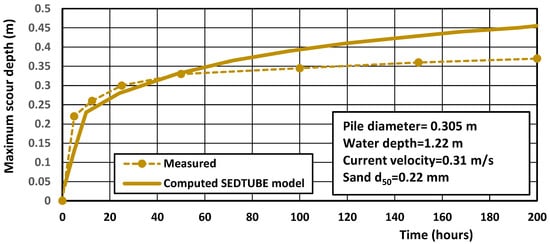
Figure 17.
Measured and computed scour depth as function of time; Sheppard test (2003) [33].
4.5. Field Case—Scour Around Pile in Tidal Flow—Scroby Sands, UK
The Barrow wind park, with 30 monopiles (Dpile = 4.2 m), was built at a site known as Scroby Sands, about 2 km off the east coast near Great Yarmouth (UK) in 2003–2004 [12,34]. The site is in relatively shallow water (7 to 15 m to MSL) and exposed to waves and strong currents in a dynamic sand bank environment (d50 = 0.26 mm). The tidal range is about 2 m. The time series of measured current speed profiles (based on ADCP data) shows values up to 1.4 m/s during the spring–neap cycle. Waves break on Scroby Sands during extreme storm events.
The scour depths were measured in March 2004, about 1 to 5 months after installation of all piles. The maximum scour depth is about 5.5 (±1.5) m in areas with a depth of 13 m to MSL. The side slopes of the scour are about 1 to 5.
The tidal cycle is represented as follows: (1) one single tide, with η1,max = 2 m, u1,max = 1.1 m/s, and T1 = 12 h, or (2) a neap–spring cycle, with η1,max = 2 m, ηw,max = 0.2 m, u1,max = 1.1 m/sm, u2,max = 0.2 m/s, and T2 = 12.4 h.
The velocity increase along the pile structure is assumed to be 1.5 [1]. The increase and decrease in the velocity along the pile at t = 3 h (maximum flood flow) are simulated by narrowing and widening the stream tube. The upstream width of the stream tube is set to b = 1 m. The depth-averaged velocity increases and decreases from 1.1 m/s to 1.65 m/s and back to 1.1 m/s (factor 1.5). The computed critical velocity is 0.43 m/s.
The turbulence coefficient is ro = 0.35. The fluid and sediment density are 1025 and 2650 kg/m3. The settling velocity is set to ws = 0.03 m/s. The bed porosity is set to 0.4. The bed roughness is set to 0.1 m. The grid size is 1 m. The time step is 60 s. The bed smoothing coefficient is 0.01. The sediment transport at the upstream boundary is set to equilibrium sand transport (default calibration coefficient = 1). The runtime for 90 days is 5 s.
Measured and computed scour depths for one single representative tide are shown in Figure 18. The measured maximum scour depth after 90 days is about the same (5.5 m) as the computed value. The time scale of maximum scour depth is about 2 months (60 days). Taking the neap–spring cycle into account, the computed maximum scour depth after 90 days is marginally smaller (<0.1 m).
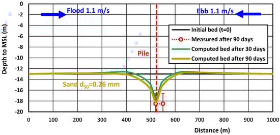
Figure 18.
Measured and computed free scour depth after 30 and 90 days; Scroby Sands (UK).
4.6. Scour Downstream of Culvert in Eastern Scheldt, The Netherlands
Üşenti (2019 [35]) described the scour downstream of a new culvert in the dike of the tidal Eastern Scheldt (The Netherlands) to allow water to flow into a natural reserve area. The structure was completed in December 2014.
A deep scour pit was generated in the bed of fine sand (d50 = 0.13 mm) within 12 days after the opening of the new structure; see Figure 19. The water depth is about 4 m. The outflow is a jet type of flow, which gradually spreads out in a lateral direction. The depth-averaged flow velocity in the center line is in the range of 1.25–1.5 m/s at the entrance, x = 0, decreasing to 0.8–1 m/s at x = 50 m and to 0.3 m/s a t x = 100 m due to lateral widening of the jet.
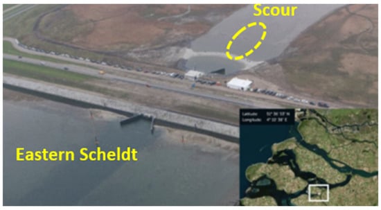
Figure 19.
Measured bathymetry downstream of culvert (see white box of inset) in dike of Eastern Scheldt (NL).
The 1D SEDTUBE model has been used to simulate the scour downstream of the culvert. The extra turbulence generated in the outflow is represented by a virtual structure on the bed with ro = 0.3. The outflow velocity is set to 1.25 and 1.5 m/s (two cases). The velocity distribution along the stream tube at t = 0 is shown in Figure 20. The computed and measured bed levels along the center line after 12 days are also shown in Figure 20. The computed maximum scour depth after 12 days is of the right order of magnitude (scour depth of about 5 m below the surrounding bed) for a mean current of 1.5 m/s in combination with ro = 0.3. The eroded sand is deposited after 60 m in the area where the current velocity decreases and the extra turbulence has decayed.
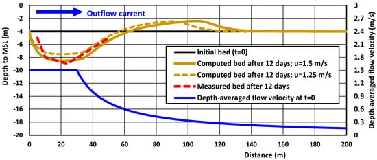
Figure 20.
Measured and computed scour pit downstream of culvert; Eastern Scheldt (NL).
4.7. Scour Downstream of Rock Berm Structure, Morecambe Bay, UK
Severe scour has been observed in recent surveys near the rock protection at the crossing of Cable A and Cable 1–2 (KP4.6 to 4.7), southwest of Heysham in Morecambe Bay, Northern Irish Sea, UK, Figure 21. Available data on seabed profiles and plan-view bathymetry at the cable crossings over the period 2006 to 2019 show the presence of a significant scour hole near the rocky cable crossing (GEO-4D, 2022 [36]).
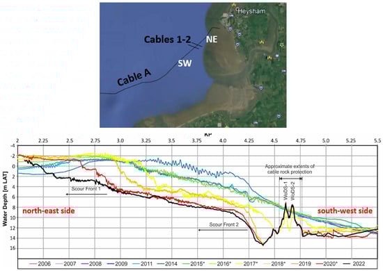
Figure 21.
Longitudinal section along Cable A; 2006–2022.
Morecambe Bay (MB) is a very dynamic and complex system, consisting of deeper channels and wide, shallow intertidal shoals and flats (sand–mud) with input from four rivers (Wyre, Lune, Kent, and Leven). More than half of the bed area of the Bay (300 km2) is exposed at LW spring tides. Morecambe Bay has the largest tidal range in the northern Irish Sea. The maximum spring tides have a range of about 10 m. Minimum neap tides have a range of about 3.5 m. Tidal currents at the mouth of the bay are typically 0.5 m/s on spring tides, increasing to 2 m/s on spring tides in the deeper channels (Lune Deep). In September–October 2022, detailed measurements of tidal currents were performed at two stations near the cable crossing. South of the cable crossing, depth-averaged tidal current velocities generally range between 1.1 m/s (flood flow to north-east) and 0.7 (ebb flow to south-west) on spring tides, reducing to between 0.4 m/s (flood) and 0.2 m/s (ebb) on neap tides. North of the cable crossing, depth-averaged tidal current velocities generally range between 1.4 m/s (flood flow) and 1.1 m/s (ebb flow) on spring tides, reducing to between 0.5 m/s (flood) and 0.3 m/s (ebb) on neap tides.
Bed samples show the presence of fine-to-medium sand in the deeper channels and silty/clayey sediments in the shallow parts. Two scour areas on the northeast and southwest side of the cable crossing were observed during surveys; see Figure 21. The scour depths on the northeast side are larger and extend over a longer area (1 to 2 km) than those on the southwest side, which can be attributed to the larger peak current velocities of the flood tide (on the order of 1.0 to 1.4 m/s during springtide) going in northeast direction.
The maximum scour depth on the northeast side (KP4.35) has developed as follows: (1) the bed was at −7 m below CD in 2014; (2) the deepest point of the bed was about −12.5 m below CD in 2017 (maximum scour depth = 5.5 m after 3 years); (3) the deepest point of the bed was about −15 m below CD in 2020 (maximum scour depth = 8 after 6 years), and (4) the deepest point of the bed was about −15 m below CD in 2022 (maximum scour depth = 8 m after 8 years). The maximum scour depth is about 8 m at about 200 m from the crossing; the scour stabilizes after 2020 due to the local equilibrium of erosion and deposition in the deepest region and/or due to the presence of more erosion-resistant layers (till or something similarly competent).
Figure 22 shows the observed and the computed maximum scour depth based on the SEDTUBE model. The computed scour depth values are of the right order of magnitude compared to the observed values after 8 years (period 2014–2022). The critical depth-averaged velocity is set to 0.6 m/s, given the presence of silty/clayey bed materials. A smaller value of the critical depth-averaged velocity of 0.3 m/s (instead of 0.6 m/s) gives a slightly deeper scour hole. The deepest scour hole is obtained for a higher value (γbh2 = 2; L2 ≅ 320 m) of the turbulence decay length. The runtime for a domain of 5 km and 8 years is only 10 s (grid size = 1 m; time step = 5 min).
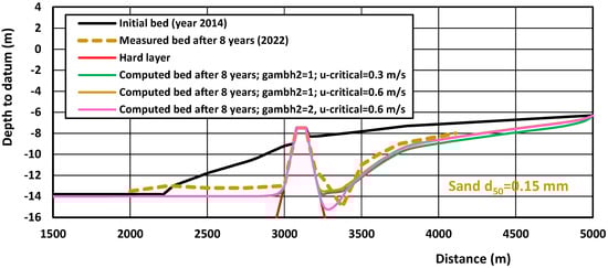
Figure 22.
Computed and observed scour depths on both sides of cable crossing.
4.8. Sedimentation in Trial Dredge Trench in Western Scheldt Estuary, The Netherlands
In 1965, a trial dredge trench was dredged perpendicular to the tidal flow in the Westerschelde (Western Scheldt estuary), a tidal estuary in the southwest part of The Netherlands [23,24,37,38,39,40,41,42]. The bed consisted of fine sand with d50 = 0.18 mm and settling velocity ws = 0.015 m/s. The peak flood and ebb velocities were 1.5 and 0.8 m/s. A typical cross-section is shown in Figure 23. Flow velocity and sand concentration measurements were carried out to estimate the suspended transport. The bed load transport was not measured. The calibration coefficient of the suspended load transport was set to 1.2 to represent the measured values. Figure 23 shows measured and computed bed levels after 22 and 80 days. The measured bed level profiles show a dominating effect of the ebb period. The computed sedimentation is in good agreement with observed values. The computed erosion near the left upper edge of the trench was not measured.
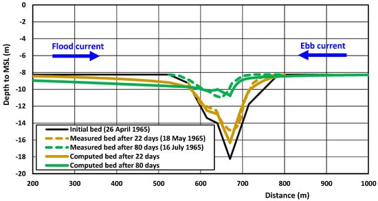
Figure 23.
Measured and computed bed levels after 22 and 80 days; trial dredge trench Western Scheldt (NL).
5. Summary, Applications, and Conclusions
A fairly simple 1D numerical model (SEDTUBE model) for the computation of sand transport rates and scour depths near structures on the seabed (berms, bed protections) is proposed, tested, and validated. Originally, this model was developed for unidirectional flow and sediment transport as an Excel tool. Recently the model was extended to tidal flow as a FORTRAN model. Furthermore, hard layers of (multiple) structures are included in the model domain. Hence, the model computes the sediment transport along the bed and over the structure.
The SEDTUBE model can predict the time evolution of the free scour depth around rock berms, bed protections, and pile-type structures, as well as the edge scour further away from the pile in unidirectional and bidirectional tidal flows (weak and strong currents) in combination with waves over a sandy sediment bed with d50 in the range between 0.2 and 2 mm. The model can represent the flow and sand transport along a stream tube with constant or variable width, including hard layers. The model is much more than a scour model; it is a universal model in the sense that it can also be used for the prediction of sedimentation in shipping channels (Section 4.8). The model is valid for sandy beds and for mud–sand beds with slight cohesive properties. A major advantage of the model is the very low computational run time (seconds for short-term predictions to minutes for long-term predictions up to 50 years), which allows the execution of many runs to assess the model sensitivity for key input parameters. A summary of the input parameter as used in the validation cases (six laboratory cases and four field cases) is presented in Table 5.
Table 5.
Summary of input parameters used in validation cases (L = laboratory; F = field; UDF = unidirectional flow; TF = tidal flow).
The laboratory cases concern scour downstream of a bed protection, a rock berm, and piles without bed protection (free scour). A bed protection or a rock berm is included in the flow domain as a hard layer. A pile is represented as a virtual structure generating turbulence (turbulence source). The increase and decrease in the flow velocity around the pile are represented by varying the width of the stream tube. The increase factor of the velocity is set to 1.5 in all cases [1,43].
The field cases refer to scour downstream of a culvert, scour around a pile, and sedimentation in a pipeline trench. In all cases, the adjustment coefficient of the suspended transport is set to 0.2 for fine-to-medium fine sand beds (porosity = 0.4; bulk density of 1600 kg/m3). The bed roughness varies in the range of 0.01 to 0.1 m, with smaller values for the laboratory cases and higher values for the field cases. When a structure is present in flow, turbulence parameters (ro, L1, L2) are specified to represent the generation and decay of extra turbulence downstream of the structure. The turbulence is represented in the model by increasing the depth-averaged flow velocity ue = (1 + r)u. The r-parameter grows to a maximum value ro over distance L1 and decays to 1 over distance L2. The values of L1 and L2 can be manipulated (calibrated) by the coefficients γbh1 and γbh2. The ro-parameter is found to be in the range of 0.2 to 0.7 for the laboratory cases as well as the field cases. The ro-value depends on the scale of the structure (berm height, pile diameter) and the strength of the flow. A value of ro = 0.7 was found in the laboratory test, with an extreme velocity of 1.64 m/s, while a value of ro = 0.5 was found for the field case with an exposed rock berm (initial height of 2.5 m; final height of 6 to 8 m) in Morecambe Bay (UK). If measured data are available, the turbulence parameters can be used as calibration parameters.
A typical application of the model is the scour near rock berms protecting offshore cables in tidal flow, with peak flow velocities of about 1 m/s in the North Sea. The bed material is medium fine sand with d50 = 0.25 mm and a settling velocity of 0.02 m/s. Figure 24 shows the computed bed profiles for a case with two rock berms at a spacing of 100 m after 3 months, 1 year, and 5 years. The hard layer (not erodible) is indicated by red lines. The depth-averaged flow velocity and the turbulence parameter (r) during the flood current (t = 3 h) of the first tide are also shown in Figure 24. The r-parameter at t = 3 h grows from 1 to 1.3 over a distance of about 100 m and then decays to 1 over a distance of 130 m.
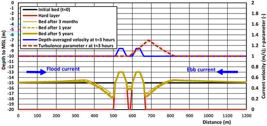
Figure 24.
Computed bed profiles after 5 years for 2 rock berms in tidal flow.
The scour depth after 3 months is about 2 m, which grows to about 2.5 m after 1 year and to 2.7 m after 5 years (runtime of 5 s). Most of the scour takes place in the first year. The scour between the rock berms grows to about 1.2 m. This example shows that the model can deal with quite complicated configurations. Given the negligible runtime (<5 s), many computations using different settings can be made to better understand the variation ranges involved.
The SEDTUBE model can also be used with confidence to predict the sedimentation of trenches and shipping channels based on the validation cases for pipeline tranches in the North Sea (NL) and in the Western Scheldt estuary (NL). In all validation cases, the calibration coefficients of the (unknown) upstream bed load and suspended load transport are in the range of 0.5 to 1.5, which is a good result given the complexity and inherent inaccuracy of sediment transport predictions.
Finally, a serious model limitation is mentioned. A key difficulty lies in estimating the coefficient of artificial turbulence. The computed scour strongly depends on the turbulence parameters involved, which are essentially empirical in nature and may vary from case to case (see Table 5), requiring calibration and sensitivity runs. More research on these turbulence-related parameters is required (future work) to improve overall model performance.
Author Contributions
Conceptualization, methodology, and writing, L.C.v.R.; Software development, K.L.M. All authors have read and agreed to the published version of the manuscript.
Funding
This research received no external funding.
Data Availability Statement
All experimental data are available on request.
Conflicts of Interest
Author L. C. van Rijn was employed by the company LVRS-Consultancy, author K. L. Meijer was employed by the company Technical Software Development. Authors declare that the research was conducted in the absence of any commercial or financial relationships that could be construed as a potential conflict of interest.
References
- Van Rijn, L.C.; Geleynse, N.; Perk, L.; Schoonhoven, D. Scour near Offshore Monopiles, Jacket-Type and Caisson-Type Structures. J. Mar. Sci. Eng. 2025, 13, 266. [Google Scholar] [CrossRef]
- Melville, B. The Physics of Local Scour at Bridge Piers. In Proceedings of the Fourth International Conference on Scour and Erosion, Tokyo, Japan, 4–8 November 2008. [Google Scholar]
- Liang, B.; Du, S.; Pan, X.; Zhang, L. Local Scour for Vertical Piles in Steady Currents: Review of Mechanisms, Influencing Factors and Empirical Equations. J. Mar. Sci. Eng. 2020, 8, 4. [Google Scholar] [CrossRef]
- Gong, E.; Chen, S.; Chen, X.; Guan, D.; Zhang, J. Large-scale experimental study on scour around both slender and large monopiles under irregular waves. Water Sci. Eng. 2025. [Google Scholar] [CrossRef]
- Garcia, K.; Jordan, C.; Melling, G.; Schendel, A.; Welzel, M.; Schlurmann, T. Scour variability across offshore wind farms (OWFs): Understanding site-specific scour drivers as a step towards assessing potential impacts on the marine environment. Wind. Energy Sci. 2025. [Google Scholar] [CrossRef]
- Cui, J.; Bao, T.; Ding, X.; Tang, C.; Li, T.; Zhou, W. Scour predictions, monitoring and protection measures for offshore wind turbines; recent advancements and insights. Ocean. Eng. 2025, 339, 122194. [Google Scholar] [CrossRef]
- Yu, H.; Zhang, Y.; Jia, J.; Zhang, J. Experimental and Numerical Study on Local Scour of Pile Group Foundations for Offshore Wind Turbines Under Wave-Current Interactions. China Ocean 2025, 39, 493–503. [Google Scholar] [CrossRef]
- Duan, B.; Wang, D.; Qin, C.; Duan, L. Local Scour Around Marine Structures: A comprehensive review of influencing factors, prediction methods, and future directions. Buildings 2025, 15, 2125. [Google Scholar] [CrossRef]
- Rudolph, D.; Raaijmakers, T.; Stam, C.J. Time-Dependent Scour Development Under Combined Current and Wave Conditions, Hindcast of Field Measurements. In Proceedings of the 4th International Conference on Scour and Erosion, Tokyo, Japan, 5–7 November 2008. [Google Scholar]
- Raaijmakers, T.C.; Van Velzen, G.; Riezebos, H.J. Dynamic Scour Prediction for Offshore Monopiles. In Proceedings of the 7th International Conference Scour and Erosion, Perth, Australia, 2–4 December 2014. [Google Scholar]
- Whitehouse, R.S.J. Marine Scour at Large Foundations. In Proceedings of the 2nd International Conference on Scour and Erosion, Singapore, 14–17 November 2004. [Google Scholar]
- Whitehouse, R.; Harris, J.; Sutherland, J.; Rees, J. An Assessment of Field Data for Scour at Offshore Wind Turbine Foundations. In Proceedings of the Fourth International Conference on Scour and Erosion, Tokyo, Japan, 5–7 November 2008. [Google Scholar]
- Whitehouse, R.; Harris, J.; Sutherland, J. Evaluating scour at marine gravity structures. HR Wallingford. ICE-Marit. Eng. 2012, 164, 143–157. [Google Scholar] [CrossRef]
- Liu, Q.; Wang, Z.; Zhang, N.; Zhao, H.; Liu, L.; Huang, K.; Chen, X. Local Scour Mechanism of Offshore Wind Power Pile Foundation Based on CFD-DEM. J. Mar. Sci. Eng. 2022, 10, 1724. [Google Scholar] [CrossRef]
- Hoffmans, G.J.C.M.; Verheij, H.J. Scour Manual; Balkema Publishing Company: Rotterdam, The Netherlands, 1997. [Google Scholar]
- Breusers, H.N.C.; Raudkivi, A.J. Scouring Hydraulic Structures Design Manual Series; CRC Press: Boca Raton, FL, USA, 2020; Volume 2, ISBN 978-1000108507. [Google Scholar] [CrossRef]
- Breusers, H.N.C. Two-Dimensional Scour in Loose Sediments; Delft Hydraulics: Delft, The Netherlands, 1967; Publ. 64. [Google Scholar]
- Breusers, H.N.C.; Nicollet, G.; Shen, H.W. Local scour around cylindrical piers. J. Hydr. Res. 1977, 15, 211–252. [Google Scholar] [CrossRef]
- Van der Meulen, T.; Vinjé, J.J. Three-Dimensional Local Scour in Non-Cohesive Sediments. In Proceedings of the 15th Congress IAHR, Sao Paulo, Brazil, 27 July–1 August 1975; Volume 2, p. B33. [Google Scholar]
- Dietz, J.W. Kolkbildung in Feinen oder Leichten Sohlmaterialien bei Strömendem Abfluss Mitteilungen Heft 155; TU: Hannover, Germany, 1969; pp. 1–121. [Google Scholar]
- Schoppman, B. Strömungs—Und Transportmechanismen Einer Fortschreitenden Auskolkung. Ph.D. Thesis, University of Karlsruhe, Karlsruhe, Germany, 1972. [Google Scholar]
- Van Rijn, L.C. Principles of Sedimentation and Erosion Engineering in Rivers, Estuaries and Coastal Seas; Aqua Publications: Amsterdam, The Netherlands, 2005. Available online: www.aquapublications.nl (accessed on 1 August 2025).
- Deltares. Sutrench-Model: Two-Dimensional Vertical Mathematical Model for Suspended Sediment Transport by Currents and Waves. In Report S488 Part IV; Deltares: Delft, The Netherlands, 1985. [Google Scholar]
- Van Rijn, L.C. Mathematical modelling of suspended sediment in nonuniform flows. J. Hydraul. Eng. ASCE 1986, 112, 433–455. [Google Scholar] [CrossRef]
- Van Rijn, L.C. Principles of Fluid Flow and Surface Waves in Rivers, Estuaries and Coastal Seas; Aqua Publications: Amsterdam, The Netherlands, 2011. Available online: www.aquapublications.nl (accessed on 1 August 2025).
- Eysink, W.; Vermaas, H. Computational Method to Estimate the Sedimentation in Dredged Channels And harbour Basins in Estuarine Environments. In Proceedings of the International Conference on Coastal and Port Engineering in Developing Countries, 1st International Association for Hydraulic Research, Colombo, Sri Lanka, 20–26 March 1983. [Google Scholar]
- Van Rijn, L.C. Unified view of sediment transport by currents and waves, I: Initiation of motion, bed roughness, and bed-load transport. J. Hydraul. Eng. 2007, 133, 649–667. [Google Scholar] [CrossRef]
- Van Rijn, L.C. Principles of Sediment Transport in Rivers, Estuaries and Coastal Seas; Aqua Publications: Amsterdam, The Netherlands, 1993. Available online: www.aquapublications.nl (accessed on 1 August 2025).
- Van Rijn, L.C. Unified view of sediment transport by currents and waves, II: Suspended transport. J. Hydraul. Eng. 2007, 133, 668–689. [Google Scholar] [CrossRef]
- Hoffmans, G.J.C.M. Concentration and Flow Velocity Measurements in a Local Scour Hole; Department of Civil Engineering, Delft University of Technology: Delft, The Netherlands, 1990; Report 4–90. [Google Scholar]
- Deltares. Systematic Study of 2D and 3D Scour Downstream of Structures (in Dutch); Deltares: Delft, The Netherlands, 1972; Report M648–863. [Google Scholar]
- Sheppard, D.M.; Miller, W. Live-Bed local pier scour experiments. J. Hydraul. Eng. ASCE 2006, 132, 635–642. [Google Scholar] [CrossRef]
- Sheppard, D.M. Large Scale and Live Bed Local Pier Scour Experiments (Phase 1); Florida Department of Transportation FDOT: Tallahassee, FL, USA, 2003; Final Report.
- Høgedal, M.; Hald, T. Scour assessment and design for scour for monopile foundations for offshore wind turbines. Cph. Offshore Wind 2005, 1–10. [Google Scholar]
- Üşenti, B. Scour Hole Formation for Lateral Non-Uniform Flow in Non-Cohesive Sediments. Master’s Thesis, Department of Civil Engineering, Delft University of Technology, Delft, The Netherlands, 2019. [Google Scholar]
- GEO-4D. Barrow Offshore Wind Farm Export cable WoDS Crossing. In Factual Survey Results Report No: P1063-DC-H015; Unit 5; RAC Estate: Faringdon, UK, 2022. [Google Scholar]
- Deltares. Numerical Model for Non-Steady Suspended Transport (in Dutch). In Report R975 Part II; Deltares: Delft, The Netherlands, 1977. [Google Scholar]
- Deltares. Computation of Siltation in Dredged Trenches. In Report R1267 Part V; Deltares: Delft, The Netherlands, 1980. [Google Scholar]
- Kerssens, P.J.M.; Prins, A.; Van Rijn, L.C. Model for suspended sediment transport. J. Hydraul. Div. ASCE 1979, 105, 461–476. [Google Scholar] [CrossRef]
- Van Rijn, L.C. Sedimentation of dredged channels by currents and waves. J. Waterw. Port Coast. Ocean. Eng. ASCE 1986, 112, 541–559. [Google Scholar] [CrossRef]
- Van Rijn, L.C.; Meijer, K.; Dumont, K.; Fordeyn, J. Practical 2DV modelling of deposition and erosion of sand and mud in dredged Channels due to currents and waves. J. Waterw. Port Coast. Ocean. Eng. 2024, 150, 04024002. [Google Scholar] [CrossRef]
- Van Rijn, L.C.; Meijer, K.; Dumont, K.; Fordeyn, J. Simulation of sand and mud transport processes in currents and waves by time-dependent 2DV model. Int. J. Sediment Res. 2024, 40, 1–14. [Google Scholar] [CrossRef]
- Wang, G. PIV-Experiment and CFD Simulation of Flow Around Cylinder. Master’s Thesis, Department of Civil Engineering, University of Texas, Austin, TX, USA, 2015. [Google Scholar]


Disclaimer/Publisher’s Note: The statements, opinions and data contained in all publications are solely those of the individual author(s) and contributor(s) and not of MDPI and/or the editor(s). MDPI and/or the editor(s) disclaim responsibility for any injury to people or property resulting from any ideas, methods, instructions or products referred to in the content. |
© 2025 by the authors. Licensee MDPI, Basel, Switzerland. This article is an open access article distributed under the terms and conditions of the Creative Commons Attribution (CC BY) license (https://creativecommons.org/licenses/by/4.0/).