Article

Radar Target Detection in Sea Clutter Based on Two-Stage Collaboration

1
Hainan Branch, Institute of Acoustics, Chinese Academy of Sciences, Haikou 570105, China
2
Lingshui, Marine Information, Hainan Observation and Research Station, Lingshui 572423, China
*
Author to whom correspondence should be addressed.
J. Mar. Sci. Eng. 2025, 13(8), 1556; https://doi.org/10.3390/jmse13081556
Submission received: 21 June 2025 / Revised: 7 August 2025 / Accepted: 12 August 2025 / Published: 13 August 2025
(This article belongs to the Section Physical Oceanography)

Abstract

Radar target detection in sea clutter aims to effectively discern the presence of maritime targets within the current radar echo. The latest detection methods predominantly rely on sophisticated deep neural networks as their underlying design framework. One major obstacle to applying these radar target-detection methods in practical scenarios is the false alarm rate. The existing methods are mostly one-stage, where after feature extraction from radar echoes, a single prediction is made to determine whether or not it contains a sea surface target, resulting in a binary classification result. In this paper, we propose a detection model with the intention of increasing the credibility of the prediction results through a two-stage confirmation process, thereby advancing the practical application of neural-based radar target-detection algorithms. Experimental findings provide compelling evidence supporting the superiority of the proposed method in terms of detection performance and robustness under different conditions, surpassing existing techniques. In light of practical deployment considerations, future efforts should be directed towards investigating the generalization capabilities of the radar detection model specifically under low sea conditions.

1. Introduction

Radar, as an active electronic detection device, has the functions of transmitting, receiving, and processing radio signals, and is commonly used for detecting and monitoring targets on the sea surface. Compared to other types of sensors, radar is widely applied due to its all-weather, all-time, and long-range working characteristics. Radar maritime target-detection technology has significant application value [1,2] in areas such as maritime safety, maritime surveillance and defense, search and rescue, and marine resource development, contributing to the protection of maritime security and effective utilization of marine resources. Therefore, radar maritime target-detection technology has become a research hotspot among scholars in the related field of radar.
Radar maritime target detection encounters a significant challenge, that is the issue of frequent false alarms. The primary cause of this challenge is the interference caused by sea clutter [3,4]. Sea clutter is characterized by non-Gaussian behavior and often exhibits sudden generation of intense echoes, known as sea spikes. Consequently, when radar attempts to process these abrupt and strong echo signals, it can result in a considerable number of false alarms. For X-band pulse compression radar, rain clutter [5] also affects the signal-to-noise ratio of received echoes. Additionally, factors like hardware aging can introduce sudden spikes of noise into radar echoes. These factors collectively impact the performance of radar target detection, resulting in an increased occurrence rate of false alarms. Hence, radar target-detection algorithms are unable to effectively serve as a sea surface warning system. In most cases, manual verification by personnel is still required to confirm the detections (as shown in Figure 1). Therefore, effectively reducing false alarms and minimizing false reports are crucial prerequisites for advancing the practical applicability of radar target-detection algorithms.
The common paradigm of existing radar target-detection algorithms is to first extract features and then perform binary classification prediction. In terms of feature extraction, many researchers have proposed a series of feature-extraction methods based on the time-frequency characteristics [6,7,8,9,10] of radar echoes. For instance, Shui et al. [6] developed a three-feature detection method for floating small targets in sea clutter based on time-frequency analysis. Xu et al. [7] obtained three polarization features from multiple polarization channel echoes. Yan et al. [8] introduced a data-driven approach using the average spectral radius. Additionally, some scholars have leveraged the powerful capabilities of deep neural networks [11,12,13,14,15,16,17], inputting either raw echoes or time-frequency features into neural networks. By utilizing their nonlinear fitting ability through supervised training, these networks automatically learn which features are most effective for classification. In Refs. [12,17], we separately explored the application prospects of CNN and LSTM, two standard structures, in radar target detection. Drawing upon the inherent characteristics of the task, we introduced adaptive modifications to the vanilla network architecture to effectively capture both global and local correlation features.
Most of the existing methods cannot reach controllable low false alarm. We believe that most existing methods belong to one-stage approaches, where the model provides results in a single prediction. In this paper, we explore a two-stage approach in order to potentially achieve better performance than one-stage methods. The contributions of this paper can be summarized as follows:
1.
This paper introduces a two-stage detection paradigm, providing a new direction for controllable false alarm in radar target detection. Experimental results also demonstrate the effectiveness of the proposed method.
2.
This paper presents a radar echo embedding module and a high-level reconstruction module. Combining these two network architectures can achieve high-level feature extraction of radar echoes.
3.
An open dataset for X-band pulse compression radar is established. We will open source these data in batches in the future.

2. Related Works

Considering the practical application, one of the main issues is the high false alarm rate of radar target-detection algorithms. Once deployed, radar surveillance systems operate continuously in all weather and conditions, making the severity of false alarms one of the critical indicators for assessing the robustness of the system. Frequent false alarms necessitate constant human verification of whether a target requires pre-warning, thus increasing labor costs. Therefore, a truly practical radar target-detection algorithm must achieve a low false alarm rate to minimize erroneous alerts as much as possible.
Early radar target-detection methods primarily revolved around Constant False Alarm Rate (CFAR) algorithms [18,19,20,21], which utilized adaptive calculations to determine detection thresholds based on the echo energy received. These algorithms were designed to maintain a consistent false alarm rate while identifying the presence of targets amidst background noise. However, despite their widespread use, CFAR algorithms often encounter significant difficulties in fulfilling predefined false alarm rate criteria, particularly in scenarios characterized by low signal-to-noise ratios, such as those influenced by sea clutter interference. This limitation hampers the overall detection performance of radar systems, revealing a critical need for more robust methodologies capable of overcoming these challenges.
In light of the limitations posed by traditional CFAR techniques, researchers have turned to statistical feature-based methods for target detection in cluttered maritime environments [6,7,8,9,10,22,23,24]. These approaches aim to harness the inherent statistical characteristics of radar echoes to improve detection accuracy and reduce false alarms. Nevertheless, the complexities of real marine environments—where diverse surface targets can manifest in varying conditions—make it challenging to manually design features that are universally applicable across different scenarios. As a result, there remains considerable scope for enhancing the effectiveness of detection algorithms through the development of more sophisticated techniques that can adapt to the idiosyncrasies of marine conditions. This gap has prompted a shift towards exploring automated approaches, particularly utilizing deep learning networks, to capture nuanced features within high-dimensional spaces effectively.
As researchers delve into the potential of deep learning for radar target detection [11,13,14,25,26,27], they recognize both its promise and its challenges. The paradigm of these methods is shown in Figure 2. Deep networks are capable of automatically learning and extracting meaningful features from complex datasets, allowing for improved differentiation between sea clutter and marine targets. However, a significant limitation of these approaches is their heavy reliance on the distribution of training samples. In practical applications, variations in the operational environment can lead to discrepancies in training data, potentially constraining the generalization performance of deep-learning models. Consequently, achieving reliable performance in real-world systems necessitates further investigation into strategies that enhance the robustness and adaptability of deep network-based detection methods, ensuring they can effectively navigate the unpredictability of maritime settings.
To address the challenges posed by distribution shifts in radar signal processing within related fields, some researchers have conducted studies on domain adaptation methods [28,29,30,31]. For example, Reference [29] proposes a domain adaptive generation-recognition network that integrates key features of measured data into the simulated data domain to improve data efficiency and quality in the scope of human activity recognition. Reference [31] employs a pre-trained model to obtain cluster centers of the source domain as prior knowledge using balanced clustering, achieving domain adaptation by fine-tuning the model through the integration of domain adaptation and self-supervised learning in the target domain. These methods also provide valuable references for the design of our model.

3. Methodology

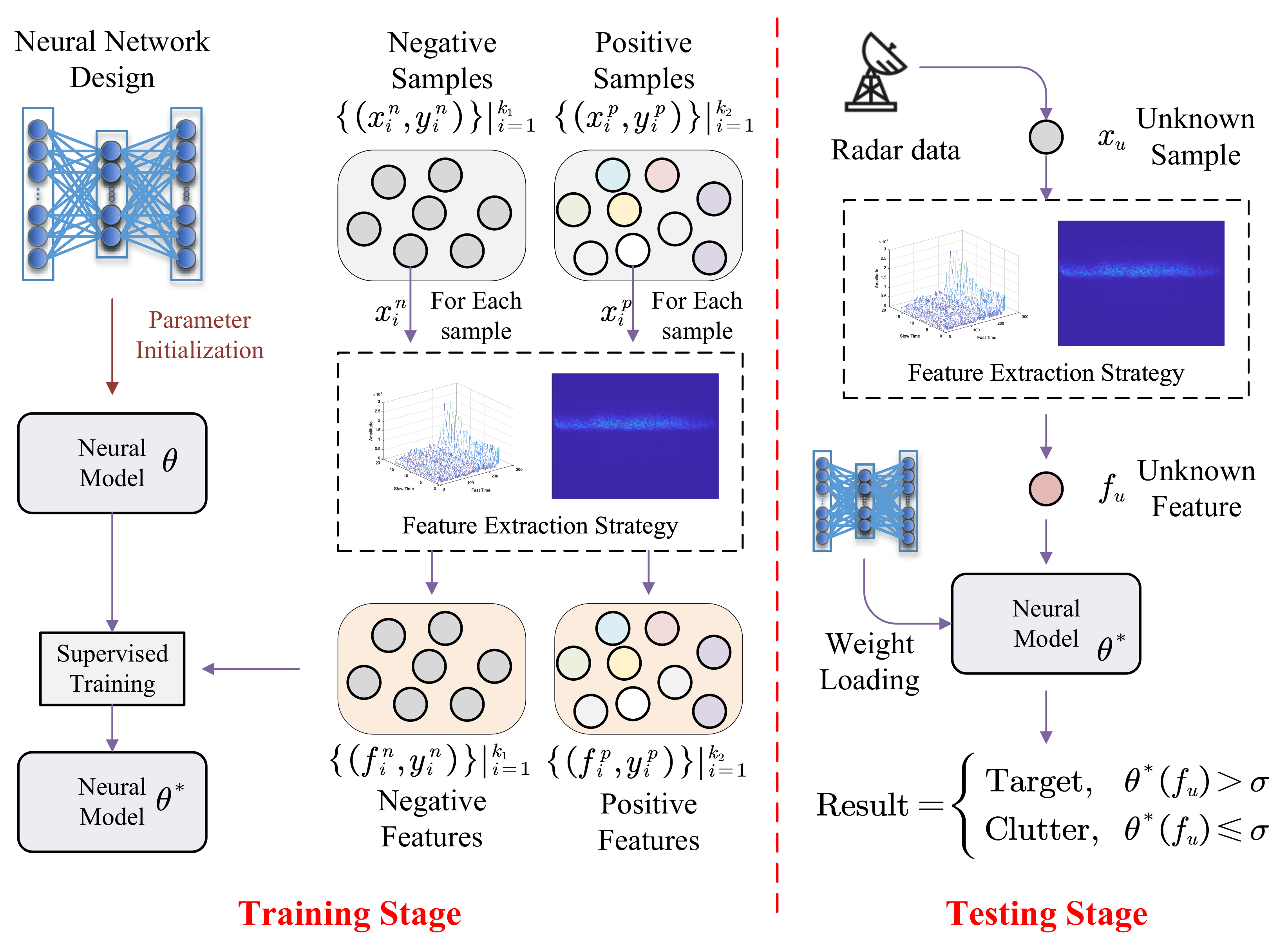
In this paper, we propose a radar target-detection method based on two-stage collaboration. The overall structure is shown in Figure 3. The following provides a detailed illustration of the proposed radar target-detection method.

3.1. Radar Target Signal Model

The model of the radar transmitted signal can generally be expressed as:
x ¯ ( t ) = a ( t ) s i n [ Ω t + θ ( t ) ]
where the variable Ω of the sine function represents the radio frequency (RF) carrier frequency, measured in rad/s; a ( t ) is the amplitude modulation of the RF carrier, which is typically a rectangular window function in pulse radar to control the signal’s on/off state; θ ( t ) denotes the phase or frequency modulation of the carrier; x ¯ ( t ) represents the signal x ( t ) , which is situated on the carrier and has not yet been demodulated. The complex baseband signal obtained after demodulation is referred to as the complex envelope of the signal waveform, given by
x ( t ) = a ( t ) e j θ ( t )
Modern pulse radars generally use digital formats to store and process radar echo data. Rather than transmitting a single pulse, the radar emits a periodic sequence of pulses. In surveillance radar applications, although a continuous sequence of pulses is transmitted, it is still processed in fixed groups of pulses. Therefore, each processing unit of the echo can be considered as a two-dimensional matrix containing two dimensions: fast time dimension (range dimension) and slow time dimension (pulse dimension).
In this echo dimensional representation, the slow time dimension represents different pulse reception periods. Combined with parameters such as antenna rotation speed, it allows for determining the angle at which the radar detects a target. The fast time dimension, on the other hand, can be used to calculate the distance to the target. The ultimate goal of radar target detection is to determine whether there is a valid maritime target present within a specific range cell of the echo.
To effectively enhance the observability of target signals, improving the signal-to-noise ratio (SNR) of the original echo signal is an important step. Common strategies include pulse integration and matched filtering. Pulse integration primarily improves the SNR by averaging multiple instances of the received signal through summation, which can be further divided into coherent integration and incoherent integration. In coherent integration, each pulse is considered a repeated pulse with the same phase as the previous ones. This method requires the accumulated signals to have stable phase information and is suitable for applications that demand high-precision measurements. In contrast, incoherent integration is a more flexible and straightforward approach, which mainly achieves pulse dimension summation by squaring the amplitude information of the received echo sequence. In the case of inputting n p pulses, the theoretical improvement in the signal-to-noise ratio for incoherent integration can be expressed by the following formula:
( S N R ) N = n p ( S N R ) O L N = n p ( S N R ) O × ( S N R ) O 1 + ( S N R ) O
where ( S N R ) O represents the SNR of a single pulse, L N is the accumulation loss in non-coherent accumulation, and the calculation here is a theoretical approximation.
Matched filtering is another means that can effectively enhance the signal-to-noise ratio, and its essence is based on the theory of maximizing the SNR of the output signal. We assume the signal at the input end of the matched filter is
x ( t ) = s ( t ) + n ( t )
where n ( t ) represents the noise component and s ( t ) represents the effective target signal.
s ( t ) = r e c t ( t T ) e x p ( j 2 π ( f 0 t + 1 2 μ t 2 ) )
By performing a Fourier transform on s ( t ) , we obtain the spectrum S ( ω ) . Assuming the transfer function of the matched filter is H ( ω ) , according to the principle of maximizing the signal-to-noise ratio, the transfer function of the filter is
H ( ω ) = K S * ( ω ) e j ω t 0
where K represents the amplitude information, and S * ( ω ) is the conjugate function of S ( ω ) . Based on the above definition, the output of the optimal matched filter can be expressed as follows:
S 0 ( ω ) = S ( ω ) H ( ω ) = K | S ( ω ) | 2 e j ω t 0
The result after transforming back to the time domain is as follows:
s 0 ( t ) = h ( t ) s ( t )

3.2. Anchor Box Extraction

The presented anchor box extraction module consists of pre-processing and candidate selection. In the pre-processing stage, the echo signals of our pulse-compression radar are processed sequentially through matched filtering and normalization operations. After this pre-processing stage, we perform candidate selection on the pre-processed radar echo data. Considering computational complexity, the specific implementation of candidate selection is the CFAR (Constant False Alarm Rate) strategy. In order to retain as many potential candidates as possible, we set the false alarm threshold parameter of CFAR to be relatively low.
In the candidate selection part, we first square the amplitude of the pre-processed radar echo data. Then, for each sampling point, a certain number of guard cells and reference cells are selected on both sides. The average value of the total number of reference cells is calculated to obtain an estimation of the background clutter power. Based on the relative magnitude between the power of the current sampling point and the average power of the reference unit, we determine whether the current point is a candidate target point. If it is determined as such, anchor box extraction is performed with the current point as the anchor point (Figure 3). The extracted anchor boxes are then passed to the next stage for fine-grained prediction to further determine whether they belong to clutter or targets.

3.3. Fine-Grained Prediction

After the preliminary extraction of anchor boxes in the previous stage, we employ a neural model to further predict whether the extracted anchor boxes contain sea surface targets. The neural network model in this paper consists of several steps: encoding the radar echo signals within the anchor boxes, reconstructing the encoded vectors using convolutional networks and attention mechanisms for high-level reconstruction, and finally obtaining prediction results by passing the reconstructed feature vectors through fully connected layers.

3.3.1. Echo Embedding

We pack all sampling points of a radar echo into a matrix X R p × r as
X = s 1 , 1 s 1 , j s 1 , d s i , 1 s i , j s i , d s p , 1 s p , j s p , d
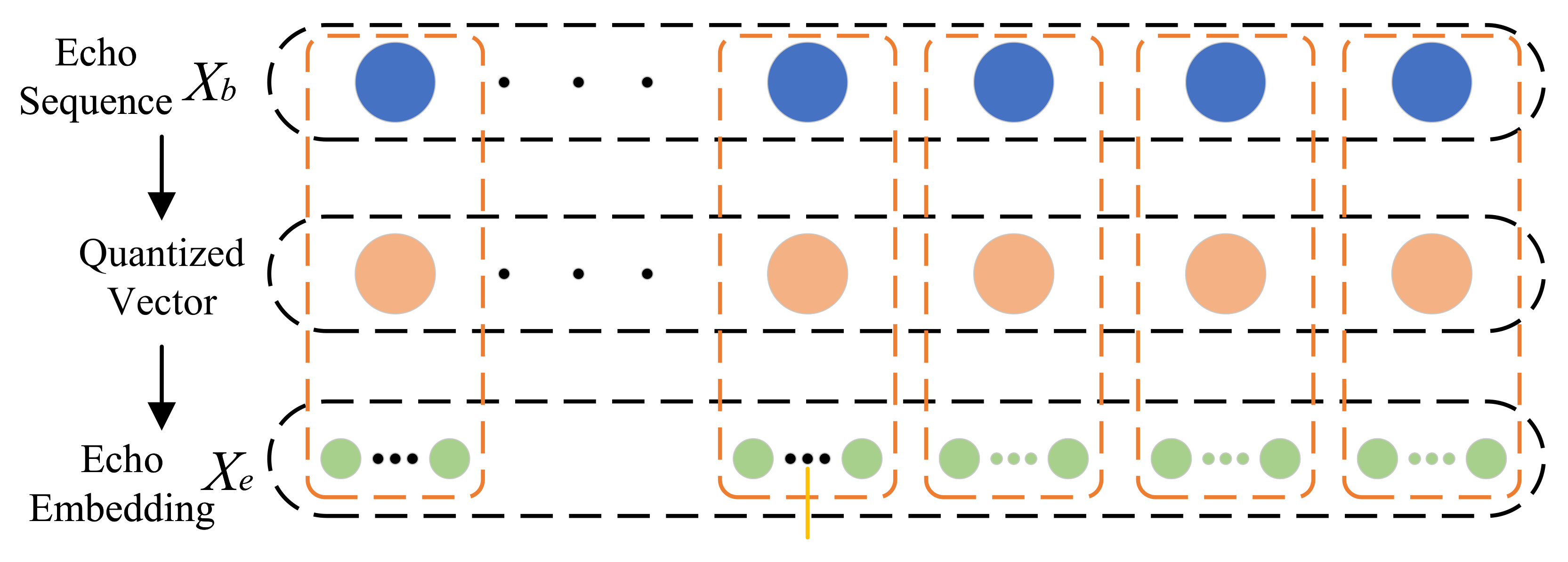
where p denotes pulse (slow time) dimension and r denotes range (fast time) dimension. We performed average pooling on X using a window size of b. This resulted in transforming X R p × r into X b R p b × r b . For each data point in X b , we quantized it using k bits, which means we fixed the value of each point to an integer in the range 1 , 2 k . In this step, we aim to reduce the data dimensionality for better computational efficiency and to simplify subsequent analysis. We constructed an embedding look-up matrix E R 2 k × d for the sampled points of the radar echoes. d is the embedding size and the value 2 k is consistent with the quantization range. Similar to the basic idea of word embedding [32], each sample point is encoded using the embedding matrix. Finally, we obtain the echo embedding X e R p b × r b × d . Taking a single pulse as an example, encoding is performed in the range dimension, and the encoding process is shown in Figure 4. After encoding, each sampled point can be represented by a d-dimensional vector.

3.3.2. High-Level Reconstruction

The high-level reconstruction module in this paper consists of two main parts: a convolutional neural network (CNN) and an attention mechanism. Its main purpose is to perform high-dimensional feature extraction on the embedded radar echoes using convolutional operations. Subsequently, an attention mechanism is employed to weight and reconstruct the extracted features. The detailed structure is illustrated in Figure 5.
As shown in the figure, our high-dimensional reconstruction module consists of two consecutive 2D convolutions with kernel sizes of 5 × 5 and a local attention mechanism. A batch normalization layer is applied after each convolution to accelerate the convergence of the network during training. The 2D convolution operation can be computed using the following formula:
x i , j ( k , l ) = c = 1 C i 1 m = 0 M i 1 n = 0 N i 1 W i , j ( m , n ) x i 1 , c ( k + m , l + n ) + b i , j
where x i , j ( k , l ) represents the output of the neuron at position ( k , l ) of the j-th feature map in the i-th convolutional layer. C i 1 is the number of feature map channels in the output of the ( i 1 ) -th convolutional layer. M i and N i are the dimensions of the 2D convolutional kernel in the i-th convolutional layer, i.e., the number of neurons in the row and column directions. W i , j ( m , n ) is the weight of the neuron at position ( m , n ) of the j-th convolutional kernel in the i-th convolutional layer. This weight is multiplied by the feature value at position ( k + m , l + n ) of the c-th feature map from the ( i 1 ) -th convolutional layer’s output. b i j is the bias value of the j-th feature map in the i-th convolutional layer. During the experimental process, we set the output channel of the first convolutional layer to 8 and the output channel of the second convolutional layer to 1. A batch normalization layer is applied after each convolution to accelerate the convergence of the network during training. The calculation process is as follows
F = N o r m ( C o n v 2 d ( N o r m ( C o n v 2 d ( X e ) ) ) )
where C o n v 2 d represents the aforementioned 2D convolution operation, N o r m denotes the batch normalization operation and F stands for the extracted features.
In the attention mechanism, we only utilize the neighboring feature points of the current feature point to generate attention weights, reflecting the concept of a local receptive field, allowing the model to focus more on the information surrounding the current position. We first perform an average pooling operation, calculated as follows:
T = A v g P o o l ( F )
A v g P o o l I j , k = 1 k m = 0 k 1 F I j , s × k + m
where A v g P o o l represents the average pooling operation, I j represents the feature index, k denotes the pooling window size, and s denotes the stripe size. Then, the input is passed through a 1D convolutional layer and a Sigmoid activation function layer to obtain the attention weight coefficients:
f w = σ ( C o n v 1 d ( T ) )
where σ represents the S i g m o i d activation function and C o n v 1 d represents the 1D convolution operation, with the following calculation formula:
x i , j k = c = 1 C i 1 m = 0 M i 1 W i , j m x i 1 , c ( k + m ) + b i , j
where x i , j k represents the feature value at position k in the j-th feature vector of the output from the i-th convolutional layer and W i , j m represents the weight of the neuron at position m in the j-th convolutional kernel of the i-th convolutional layer. This weight value is multiplied by the feature value at position ( k + m ) in the c-th feature vector of the output from the ( i 1 ) -th convolutional layer. b i , j is the bias value of the j-th feature vector in the i-th convolutional layer, M i is the size of the 1D convolutional kernel in the i-th convolutional layer, and ( c i 1 ) is the number of channels in the output feature vectors of the ( i 1 ) -th convolutional layer. Finally, the weight coefficients are multiplied pointwise with the high-dimensional features to obtain the feature information. The calculation process is as follows:
L = f w F

3.3.3. Linear Prediction

The linear prediction module consists of a fully connected layer and a sigmoid activation function, which performs the prediction on whether the input feature information L is a real target. In our training network, we use cross-entropy to compute the training loss. The calculation formula is as follows:
L o s s = i = 1 n y i l o g y i ^
where n is the total number of samples, y i ( 0 , 1 ) represents the ground truth of the i-th sample and y i ^ ( 0 , 1 ) denotes the prediction result. The network parameters are updated through backpropagation algorithm based on the obtained loss value.

4. Experiments and Discussions

4.1. Experimental Settings

4.1.1. Radar Deployment

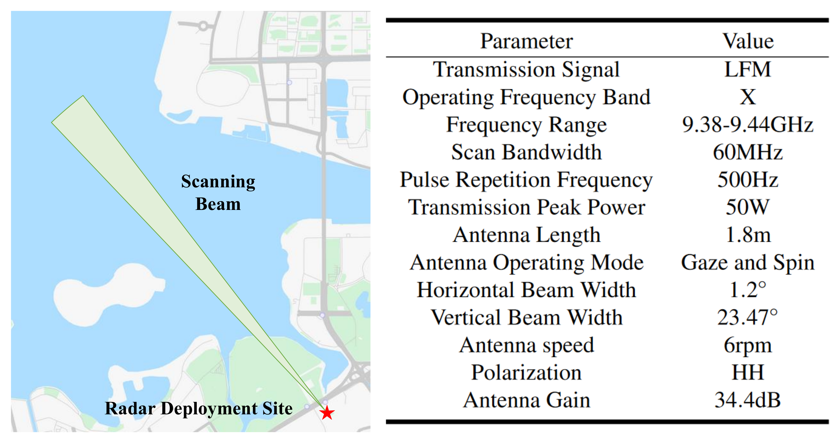
In 2023, we deployed an X-band pulse compression radar along the coast of Haikou in Hainan Province, China (Qiongzhou Strait), for maritime observation. We collected sea clutter and target-measured samples as our dataset for research on maritime target detection. The actual deployment location of our radar is shown in Figure 6.

4.1.2. Dataset Description

We have conducted long-term monitoring in the southern waters of China using X-band radar. The obtained echoes were manually annotated based on AIS (Automatic Identification System) and camera information. We collected data (as shown in Figure 7) in February, March, April, and July 2023, The ocean weather during the data collection is shown in Table 1. The data from February and March were used as the training set, while the data from April served as the validation set. As for the data from July, since it was more abundant, it was divided into three subsets based on different time periods, namely D1, D2, and D3. Our training set consists of 208,000 echo samples, while our validation set consists of 12,000 samples. As for the test set, each subset has approximately 100,000 samples in total.

4.1.3. Comparison Algorithms

To evaluate the performance of the proposed method in this paper, we selected three different detection methods as comparisons. These three methods are CA-CFAR, GO-CFAR, CA [12] and DBL [16]. Our network model is implemented in the PyTorch 1.8.1 framework and we trained and tested the model on a Geforce RTX 2080Ti GPU. During training, we used Adam as the optimizer with a learning rate of 1 × 10 3 . The chosen loss function is binary cross-entropy. We trained the network for 50 epochs with a batch size of 16.

4.2. Ablation Study

In this section, we conducted ablation experiments to discuss the contributions of different parts of the entire method to detection performance. Our approach in this paper is a two-stage method, where in the first stage we obtain candidate anchor boxes, and in the second stage, we perform further feature extraction and classification on these anchor boxes. In this section, we mainly performed ablation on the model structure involved in the second part. The experimental results are shown in Table 2. In the ablation experiments, we mainly considered the feature extraction and classification capabilities of the model. Therefore, we chose accuracy as the evaluation metric. Through experiments 1 , 2 , and 3 , we have verified the effectiveness of our overall network structure. And through experiments 4 , 5 , and 6 , we have validated the effectiveness of the parameter combination consisting of a block window size of 2 × 2 , a quantization interval of 2048, and an embedding dimension of 32 in the echo embedding stage.

4.3. Detection Performance Analysis

To validate the practical detection performance of our proposed two-stage detection algorithm, we conducted thorough testing using the dataset described in the previous section. The used evaluation metrics are detection probability (recall), false alarm rate, and precision. The experimental results are shown in Table 3. We calculated the corresponding metrics for each of the three different subsets separately, which are presented in the corresponding table.
From the table, it is evident that the method proposed in this paper exhibits significant superiority. Our approach has achieved optimality in both recall and precision metrics. Specifically, our method surpasses the 90% threshold in terms of precision across all three subsets. In the D2 subset, the DBL algorithm achieves only 76.45% precision, whereas the two CFAR-based algorithms achieve a precision rate below 40%. In contrast, our method achieves a precision rate of 90.17%, effectively reducing false positives. With respect to target-detection capability, our method attains a recall rate of 99.09% in the D2 subset, surpassing the DBL algorithm by 7.19% and the CA-CFAR algorithm by 18.00%. Across all three subsets, our method consistently exceeds a recall rate of 93%. Regarding false alarm rates, our method does not reach optimality across all subsets. For instance, in the D3 subset, the DBL algorithm has a false alarm rate of 0.08%, while ours stands at 0.57%. Nevertheless, overall, our method still falls within an acceptable range. Therefore, it can be concluded that, compared to the comparison algorithms, the proposed method exhibits optimal performance.
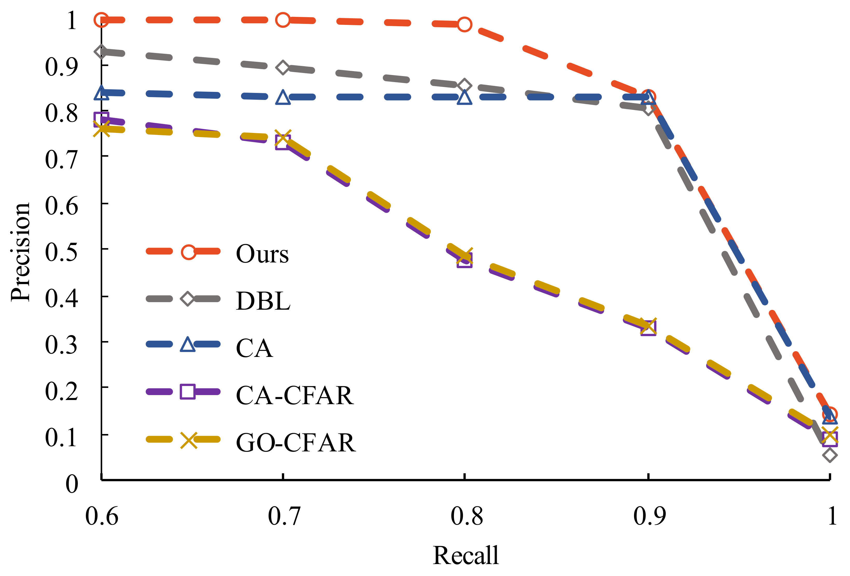
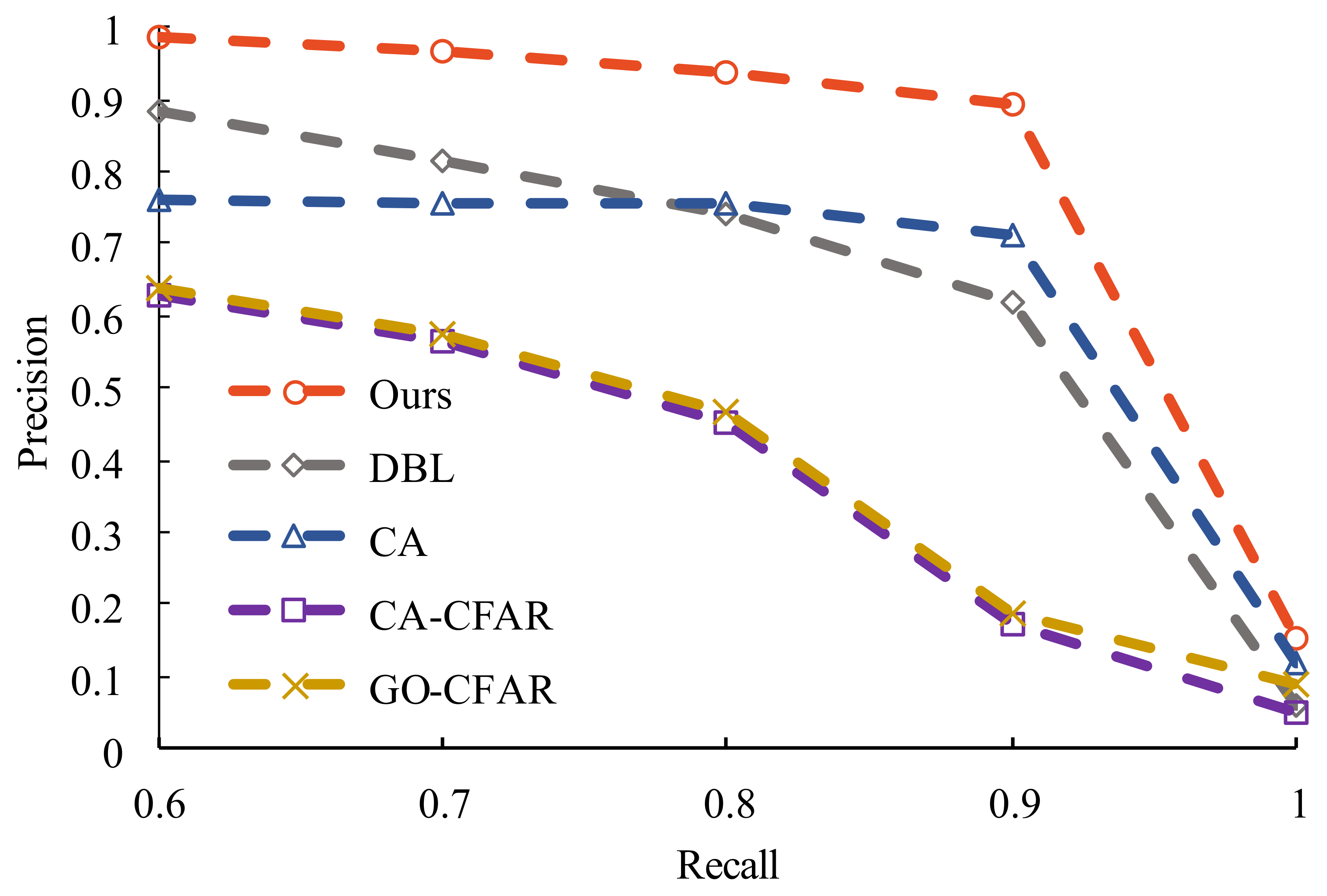
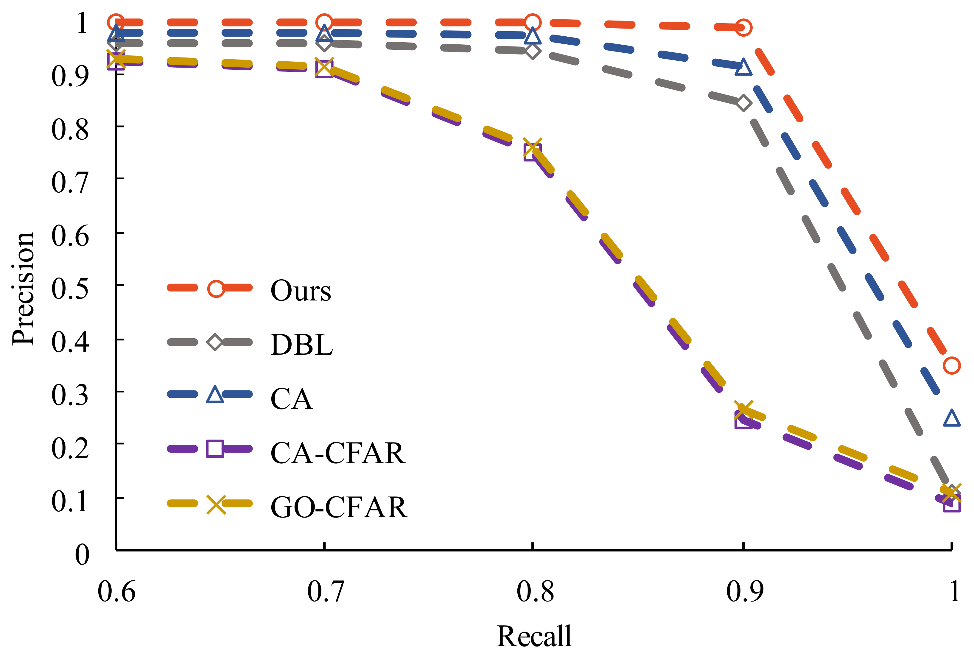
To further evaluate the detection performance of our method, we adjusted the classification threshold of the detection model and plotted the precision–recall curve as shown in Figure 8, Figure 9 and Figure 10. We believe that in practical application scenarios, it is challenging to calculate the false alarm rate because we have difficulty determining the exact number of “negative samples”. We can only know how many targets the detection algorithm currently detects and then confirm how many are true targets and how many are false targets. Therefore, we believe that compared to other methods, the precision–recall curve is a more suitable evaluation metric for assessing the performance of radar target-detection algorithms.
According to the curves in Figure 8, Figure 9 and Figure 10, our method demonstrates significant advantages. It achieves the best performance in all three subsets. In subset D2, when the recall reaches 90%, our method achieves a precision rate of 89.05%, compared to only 63.76% for DBL, which is 25.29% lower than our method. The precision rates of the two CFAR algorithms are only around 20%. Additionally, in subsets D1 and D3, our method also achieves satisfactory detection performance with precision rates of 83.14% and 99.13%, respectively, when a recall rate of 90% is required. These results indicate that our method excels in both recall and precision, outperforming other methods. It provides a reliable solution for target-detection tasks. At the same time, we plotted the ROC curves of detection accuracy for different algorithms under various false alarm rates, as shown in Figure 11. It is evident from the figure that while the DBL algorithm performs well, there is still a notable gap compared to our proposed method. The proposed algorithm consistently outperforms the comparison algorithms even under different false alarm rates.
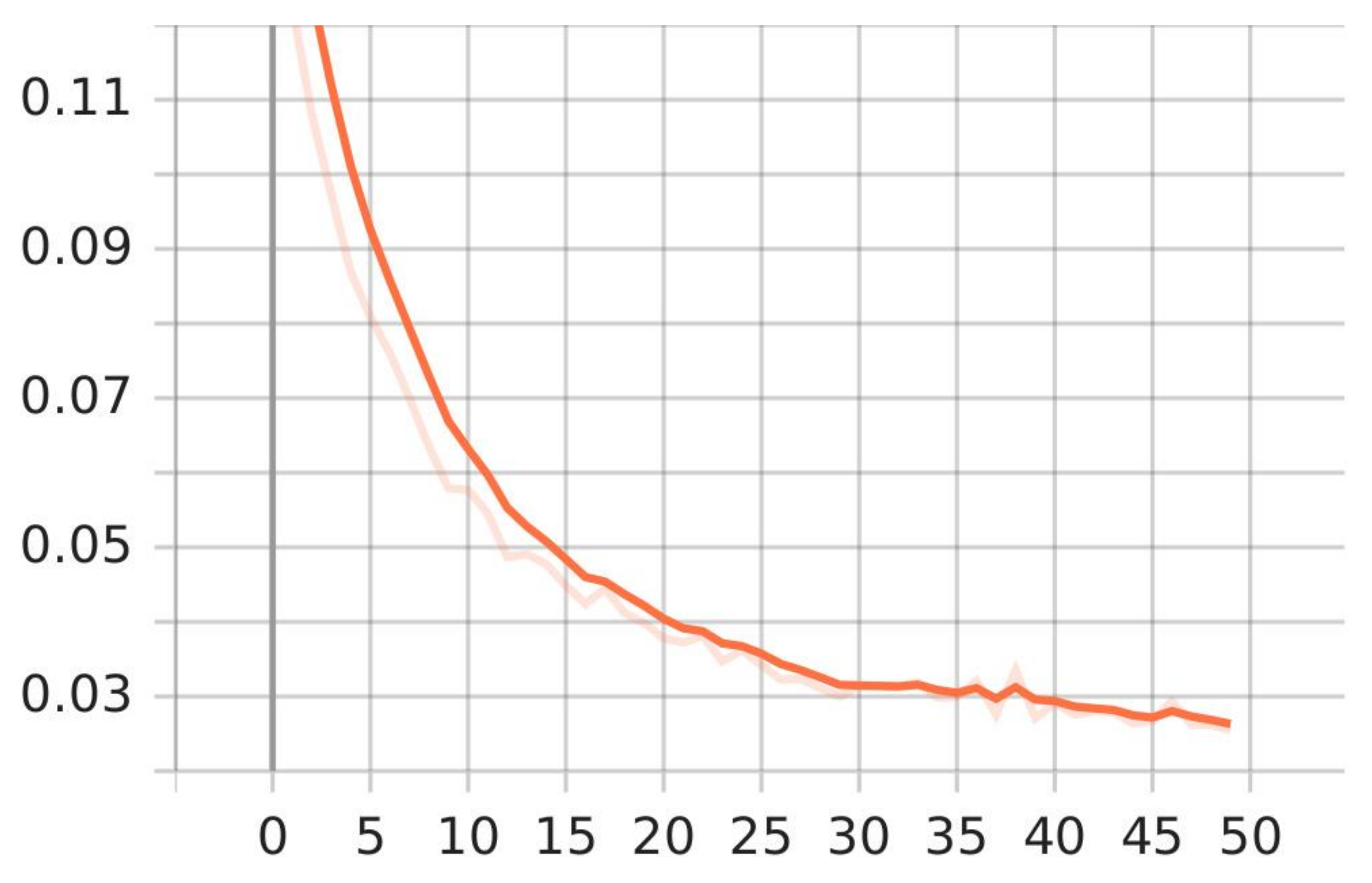
The loss curves of the training and validation procedure are presented in Figure 12. The result indicates that our model gradually converges on the training data and effectively learns appropriate feature representations and patterns from the training data. Besides, we employed the t-SNE algorithm [34] to visualize the output features generated by these methods. The results are presented in Figure 13.

5. Conclusions

This study introduces an innovative two-stage detection framework that integrates an echo embedding module and a high-level reconstruction mechanism, achieving comprehensive improvements in precision, detection probability, and false alarm rate under complex sea clutter conditions, particularly maintaining stable detection performance (0.28% false alarm rate and 99.08% detection probability) in low SNR environments. Future research will focus on constructing a multi-modal maritime target database using X-band pulse-compression radar, advancing key technologies including physics-constrained deep-learning architectures, optimized lightweight real-time processing models, and integrated multi-radar collaborative detection systems.

Author Contributions

Conceptualization, J.W.; methodology, J.W. and T.X.; software, T.X.; validation, J.W. and P.L.; investigation, J.W. and P.L.; resources, P.L.; data curation, T.X.; writing—original draft, J.W. and T.X. All authors have read and agreed to the published version of the manuscript.

Funding

This work was supported in part by Hainan Province Science and Technology Special Fund under Grant ZDYF2025SHFZ058, and in part by Youth Innovation Promotion Association, Chinese Academy of Sciences under Grant 2022022, and in part by South China Sea Nova project of Hainan Province under Grant NHXXRCXM202340, and in part by Haikou Key Science and Technology Project under Grant 2024020.

Data Availability Statement

The data that support the findings of this study are available on request from the corresponding author upon reasonable request.

Conflicts of Interest

The authors declare no conflicts of interest.

References

  1. Xu, S.; Zhu, J.; Jiang, J.; Shui, P. Sea-Surface Floating Small Target Detection by Multifeature Detector Based on Isolation Forest. IEEE J. Sel. Top. Appl. Earth Obs. Remote Sens. 2021, 14, 704–715. [Google Scholar] [CrossRef]
  2. Yan, K.; Bai, Y.; Wu, H.C.; Zhang, X. Robust Target Detection Within Sea Clutter Based on Graphs. IEEE Trans. Geosci. Remote Sens. 2019, 57, 7093–7103. [Google Scholar] [CrossRef]
  3. Liu, N.; Dong, Y.; Wang, G.; Ding, H.; Huang, Y.; Guan, J.; Chen, X.; He, Y. Sea-detecting X-band radar and data acquisition program. J. Radars 2019, 8, 656. [Google Scholar]
  4. Rosenberg, L. Sea-Spike Detection in High Grazing Angle X-Band Sea-Clutter. IEEE Trans. Geosci. Remote Sens. 2013, 51, 4556–4562. [Google Scholar] [CrossRef]
  5. Huang, W.; Liu, X.; Gill, E.W. Ocean Wind and Wave Measurements Using X-Band Marine Radar: A Comprehensive Review. Remote Sens. 2017, 9, 1261. [Google Scholar] [CrossRef]
  6. Shui, P.L.; Li, D.C.; Xu, S.W. Tri-feature-based detection of floating small targets in sea clutter. IEEE Trans. Aerosp. Electron. Syst. 2014, 50, 1416–1430. [Google Scholar] [CrossRef]
  7. Xu, S.; Zheng, J.; Pu, J.; Shui, P. Sea-Surface Floating Small Target Detection Based on Polarization Features. IEEE Geosci. Remote Sens. Lett. 2018, 15, 1505–1509. [Google Scholar] [CrossRef]
  8. Yan, Y.; Wu, G.; Dong, Y.; Bai, Y. Floating Small Target Detection in Sea Clutter Using Mean Spectral Radius. IEEE Geosci. Remote Sens. Lett. 2022, 19, 4023405. [Google Scholar] [CrossRef]
  9. Chen, X.; Guan, J.; Bao, Z.; He, Y. Detection and Extraction of Target With Micromotion in Spiky Sea Clutter Via Short-Time Fractional Fourier Transform. IEEE Trans. Geosci. Remote Sens. 2014, 52, 1002–1018. [Google Scholar] [CrossRef]
  10. Bi, X.; Guo, S.; Yang, Y.; Shu, Q. Adaptive Target Extraction Method in Sea Clutter Based on Fractional Fourier Filtering. IEEE Trans. Geosci. Remote Sens. 2022, 60, 5115609. [Google Scholar] [CrossRef]
  11. Chen, X.; Su, N.; Huang, Y.; Guan, J. False-Alarm-Controllable Radar Detection for Marine Target Based on Multi Features Fusion via CNNs. IEEE Sens. J. 2021, 21, 9099–9111. [Google Scholar] [CrossRef]
  12. Wang, J.; Li, S. Maritime Radar Target Detection in Sea Clutter Based on CNN with Dual-Perspective Attention. IEEE Geosci. Remote Sens. Lett. 2023, 20, 3500405. [Google Scholar] [CrossRef]
  13. Su, N.; Chen, X.; Guan, J.; Huang, Y. Maritime Target Detection Based on Radar Graph Data and Graph Convolutional Network. IEEE Geosci. Remote Sens. Lett. 2022, 19, 4019705. [Google Scholar] [CrossRef]
  14. Chen, S.; Feng, C.; Huang, Y.; Chen, X.; Li, F. Small Target Detection in X-Band Sea Clutter Using the Visibility Graph. IEEE Trans. Geosci. Remote Sens. 2022, 60, 5115011. [Google Scholar] [CrossRef]
  15. Qu, Q.; Wang, Y.L.; Liu, W.; Li, B. A False Alarm Controllable Detection Method Based on CNN for Sea-Surface Small Targets. IEEE Geosci. Remote Sens. Lett. 2022, 19, 4025705. [Google Scholar] [CrossRef]
  16. Wan, H.; Tian, X.; Liang, J.; Shen, X. Sequence-Feature Detection of Small Targets in Sea Clutter Based on Bi-LSTM. IEEE Trans. Geosci. Remote Sens. 2022, 60, 4208811. [Google Scholar] [CrossRef]
  17. Wang, J.; Li, S. SALA-LSTM: A novel high-precision maritime radar target detection method based on deep learning. Sci. Rep. 2023, 13, 12125. [Google Scholar] [CrossRef]
  18. Zhao, W.; Liu, W.; Jin, M. Spectral Norm Based Mean Matrix Estimation and Its Application to Radar Target CFAR Detection. IEEE Trans. Signal Process. 2019, 67, 5746–5760. [Google Scholar] [CrossRef]
  19. Maali, A.; Mesloub, A.; Djeddou, M.; Mimoun, H.; Baudoin, G.; Ouldali, A. Adaptive CA-CFAR threshold for non-coherent IR-UWB energy detector receivers. IEEE Commun. Lett. 2009, 13, 959–961. [Google Scholar] [CrossRef]
  20. Gao, G.; Liu, L.; Zhao, L.; Shi, G.; Kuang, G. An Adaptive and Fast CFAR Algorithm Based on Automatic Censoring for Target Detection in High-Resolution SAR Images. IEEE Trans. Geosci. Remote Sens. 2009, 47, 1685–1697. [Google Scholar] [CrossRef]
  21. Messali, Z.; Soltani, F.; Sahmoudi, M. Robust radar detection of CA, GO and SO CFAR in Pearson measurements based on a non linear compression procedure for clutter reduction. Signal Image Video Process. 2008, 2, 169–176. [Google Scholar] [CrossRef]
  22. Xiang, J.; Lv, X.; Fu, X.; Yun, Y. Detection and Estimation Algorithm for Marine Target With Micromotion Based on Adaptive Sparse Modified-LV’s Transform. IEEE Trans. Geosci. Remote Sens. 2022, 60, 5108617. [Google Scholar] [CrossRef]
  23. Gao, C.; Tao, R.; Kang, X. Weak Target Detection in the Presence of Sea Clutter Using Radon-Fractional Fourier Transform Canceller. IEEE J. Sel. Top. Appl. Earth Obs. Remote Sens. 2021, 14, 5818–5830. [Google Scholar] [CrossRef]
  24. Li, Y.; Xie, P.; Tang, Z.; Jiang, T.; Qi, P. SVM-Based Sea-Surface Small Target Detection: A False-Alarm-Rate-Controllable Approach. IEEE Geosci. Remote Sens. Lett. 2019, 16, 1225–1229. [Google Scholar] [CrossRef]
  25. Jing, H.; Cheng, Y.; Wu, H.; Wang, H. Radar Target Detection With Multi-Task Learning in Heterogeneous Environment. IEEE Geosci. Remote Sens. Lett. 2022, 19, 4021405. [Google Scholar] [CrossRef]
  26. Xi, C.; Liu, R. Detection of Small Floating Target on Sea Surface Based on Gramian Angular Field and Improved EfficientNet. Remote Sens. 2022, 14, 4364. [Google Scholar] [CrossRef]
  27. Su, N.; Chen, X.; Guan, J.; Li, Y. Deep CNN-Based Radar Detection for Real Maritime Target Under Different Sea States and Polarizations. In Proceedings of the Cognitive Systems and Signal Processing—4th International Conference, ICCSIP 2018, Beijing, China, 29 November–1 December 2018; Revised Selected Papers, Part II. Springer: Berlin/Heidelberg, Germany, 2018; Volume 1006, pp. 321–331. [Google Scholar]
  28. Si, X.; Zhang, C.; Li, S.; Liang, J. Source-free domain adaptation for unsupervised radar-based human activity recognition. Pattern Recognit. 2026, 169, 111866. [Google Scholar] [CrossRef]
  29. Hu, Y.; Yang, X.; Xia, Z.; Xu, F. Human Activity Recognition Trained on Simulated Millimeter-Wave Radar Data With Domain Adaptation. IEEE Trans. Instrum. Meas. 2025, 74, 2525513. [Google Scholar] [CrossRef]
  30. Hernangómez, R.; Bjelakovic, I.; Servadei, L.; Stanczak, S. Unsupervised Domain Adaptation across FMCW Radar Configurations Using Margin Disparity Discrepancy. In Proceedings of the 30th European Signal Processing Conference, EUSIPCO 2022, Belgrade, Serbia, 29 August–2 September 2022; IEEE: Piscataway, NJ, USA, 2022; pp. 1566–1570. [Google Scholar]
  31. Liu, J.; Zeng, D.; Li, L.; Lin, H.; Tian, X. Source-Free Domain Adaptation for Millimeter Wave Radar Based Human Activity Recognition. In Proceedings of the IEEE International Conference on Acoustics, Speech and Signal Processing, ICASSP 2024, Seoul, Republic of Korea, 14–19 April 2024; IEEE: Piscataway, NJ, USA, 2024; pp. 7120–7124. [Google Scholar] [CrossRef]
  32. Wang, S.; Zhou, W.; Jiang, C. A survey of word embeddings based on deep learning. Computing 2020, 102, 717–740. [Google Scholar] [CrossRef]
  33. OpenStreetMap. Available online: https://www.openstreetmap.org/ (accessed on 5 May 2024).
  34. Van der Maaten, L.; Hinton, G. Visualizing Data using t-SNE. J. Mach. Learn. Res. 2008, 9, 2579–2605. [Google Scholar]
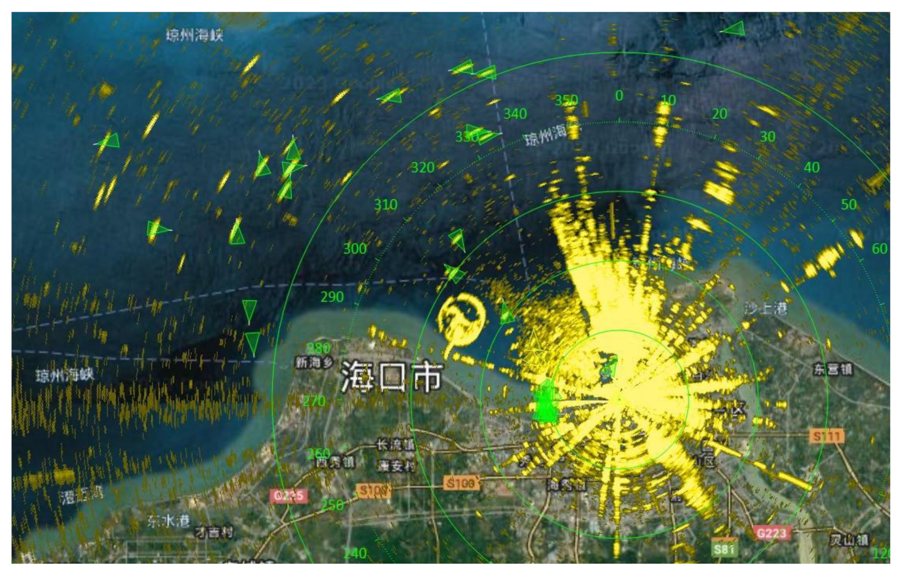
Figure 1. The maritime surveillance system deployed in the Qiongzhou Strait. The yellow part in the figure represents the detected targets. The green triangle represents the AIS information of the ship. There are many unverified targets in the figure.
Jmse 13 01556 g001
Figure 2. Paradigm of neural-based methods.
Jmse 13 01556 g002
Figure 3. The overall structure of our proposed detection method. It consists of two stage: anchor box extraction and fine-grained prediction.
Jmse 13 01556 g003
Figure 4. The encoding process diagram.
Jmse 13 01556 g004
Figure 5. The structure of high-level reconstruction module. 5 × 5 denotes the kernel size of 2D convolution. “(8)” and “(1)” means the number of convolution filters (output channel). “Norm” denotes the batch normalization layer.
Jmse 13 01556 g005
Figure 6. Sea observation scenario and the operation parameter of X-band pulse-compression radar. The map is obtained from OpenStreetMap [33]. The data of OpenStreetMap is available under the Open Database License.
Jmse 13 01556 g006
Figure 7. Typical samples for clutter (left) and target (right).
Jmse 13 01556 g007
Figure 8. The precision–recall curve for five different target-detection methods on subset D1.
Jmse 13 01556 g008
Figure 9. The precision–recall curve for five different target-detection methods on subset D2.
Jmse 13 01556 g009
Figure 10. The precision–recall curve for five different target-detection methods on subset D3.
Jmse 13 01556 g010
Figure 11. ROC curves of different algorithms.
Jmse 13 01556 g011
Figure 12. The loss curve of training set and validation set. In the two curves, the darker color represents the training set curve, while the lighter color represents the validation set curve. The x-axis represents the number of training epochs.
Jmse 13 01556 g012
Figure 13. Visualization results of features based on t-SNE [34]. This figure demonstrates the high-dimensional classification capability of our neural model for target samples and clutter samples.
Jmse 13 01556 g013
Table 1. Ocean weather conditions during data collection.
MonthMostly Cloudy/SunnyThunderstorm/RainWind Speed
February15 days13 days20–49 km/h
March23 days8 days29–38 km/h
April13 days17 days20–38 km/h
July15 days16 days20–49 km/h
Table 2. Experimental results of ablation study.
IndexModel VariantAccuracy
♯1Remove echo embedding module86.06%
♯2Remove high-level reconstruction module94.55%
♯3Only linear prediction module88.47%
♯4Change embedding size to 6495.18%
♯5Change the quantification interval to 409695.41%
♯6Change the block size to 3×394.79%
♯7The whole method95.42%
Table 3. FAR, DP, and precision of detection methods.
MetricDetection
Method
Dataset
D1D2D3
PrecisionCA-CFAR34.29%31.75%74.33%
GO-CFAR40.75%39.58%80.45%
CA [12]50.38%48.03%73.99%
DBL [16]87.06%76.45%96.48%
Ours92.65%90.17%96.78%
Recall
(DP)
CA-CFAR91.43%81.08%85.19%
GO-CFAR80.00%78.38%81.48%
CA [12]98.91%98.34%94.57%
DBL [16]91.43%91.89%88.89%
Ours97.14%99.08%93.83%
FARCA-CFAR2.99%3.46%2.65%
GO-CFAR2.92%3.37%2.58%
CA [12]1.02%1.25%0.71%
DBL [16]0.16%0.35%0.08%
Ours0.43%0.28%0.57%
Disclaimer/Publisher’s Note: The statements, opinions and data contained in all publications are solely those of the individual author(s) and contributor(s) and not of MDPI and/or the editor(s). MDPI and/or the editor(s) disclaim responsibility for any injury to people or property resulting from any ideas, methods, instructions or products referred to in the content.