Article

The Effect of Non-Breaking Wave Mixing on Ocean Modeling in the South China Sea

1
State Key Laboratory of Physical Oceanography, Ocean University of China, 238 Songling Road, Qingdao 266100, China
2
Department of Infrastructure Engineering, University of Melbourne, Parkville, VIC 3010, Australia
3
Institute of Atmospheric Physics, Chinese Academy of Sciences, 40 Huayanli, Beijing 100029, China
*
Author to whom correspondence should be addressed.
J. Mar. Sci. Eng. 2025, 13(8), 1548; https://doi.org/10.3390/jmse13081548
Submission received: 8 July 2025 / Revised: 6 August 2025 / Accepted: 7 August 2025 / Published: 12 August 2025
(This article belongs to the Section Physical Oceanography)

Abstract

This study investigates the wave-induced vertical mixing mechanism and systematically compares the application of two non-breaking wave parameterization schemes (Bv and Pw) in oceanic numerical simulations of the South China Sea, according to two key physical variables: sea surface temperature (SST) and the vertical mixing coefficient. The goal is to explore the effects of different parameterization methods on the upper-ocean temperature distribution in the South China Sea. The results indicate that although both schemes enhance vertical mixing in the upper ocean, they do so through different mechanisms. The Bv scheme directly increases the vertical mixing coefficient, demonstrating significantly stronger mixing intensity, while the Pw scheme impacts mixing indirectly by modulating turbulent kinetic energy generation, resulting in comparatively weaker mixing. SST simulation results show that the Bv scheme is more effective in reducing SST in both winter and summer, with broader spatial improvements. Further analysis of the mixing coefficient confirms that, compared to the Pw scheme, the Bv scheme not only strengthens surface mixing but also penetrates deeper into the water column.

1. Introduction

The mixed layer is typically located in the upper part of the oceanic boundary layer, with the thermocline—characterized by a pronounced vertical temperature gradient—beneath it. As the mixed layer connects the upper ocean to the atmospheric boundary layer at the base of the troposphere, it plays a critical intermediary role in the exchange of mass, momentum, and heat. This makes it a key component in the coupling between oceanic physical processes and atmospheric dynamics. Due to the influence of various physical mechanisms, the temporal and spatial variability of the mixed layer is highly complex, posing challenges for accurate characterization through observations and numerical modeling. From a dynamical perspective, the primary controlling factors of mixed layer depth can be categorized into two main types: (1) turbulent mixing processes in the upper ocean and (2) buoyancy fluxes at the air-sea interface [1,2,3,4,5]. These two factors critically influence the formation and evolution of the mixed layer structure by altering the stability and energy distribution of surface waters.
Although wave breaking is considered the primary cause of local wave energy dissipation, the turbulent kinetic energy it generates is confined to the surface layer, with its vertical scale proportional to wave height [6,7]. Surface ocean waves can also induce mixing through wave–turbulence interactions, referred to as non-breaking wave-induced mixing or wave-driven mixing [8,9,10,11]. In contrast to the mixing caused by wave breaking, the turbulence generated by non-breaking waves is linked to orbital motion within the waves and can produce eddies on spatial scales similar to the wavelength [12]. The concept of non-breaking wave mixing was originally based on a hypothesis proposed by Jeffreys [13], which suggested that waves primarily generate turbulence through velocity shear near the surface, which gradually weakens with depth. Buccini et al. [14] investigated the spatial distribution of arsenic contamination at the seabed of Bagnoli Bay in southern Italy using a particle tracking numerical modeling approach. The study explicitly considered the effects of wave-induced vertical mixing and applied seasonally varying vertical mixing coefficients, thereby enabling a more accurate reconstruction of arsenic transport pathways within both the upper and lower layers of the seabed sediments.
Recent studies have increasingly focused on how various wave mixing parameterizations affect the upper ocean. Standalone ocean circulation models often underestimate the thickness of the upper mixed layer when simulating the distribution of ocean temperature and salinity [15,16]. This deficiency has been primarily attributed to the lack of representation of non-breaking wave-induced mixing in the models. Incorporating non-breaking wave mixing has proven essential for improving upper ocean mixing and is therefore crucial in ocean model computations [8]. Qiao et al. [8] introduced the vertical viscosity term Bv into the Princeton Ocean Model (POM) to assess the impact of non-breaking wave-induced mixing. Their results showed that such mixing has a strong influence during winter in regions north of 30° N in the North Pacific and North Atlantic. Aijaz et al. [17] incorporated the non-breaking wave mixing parameter Pw into the POM model and the WAVEWATCH-III (WW3) model to conduct a series of numerical experiments examining its impact on the upper ocean during extreme typhoon events. The results indicated that non-breaking wave-induced mixing can lower sea surface temperatures and deepen the mixed layer. Their results demonstrated that non-breaking wave-induced mixing played an important role in restoring mixed-layer heat content, particularly in the peripheral and trailing stages of the typhoon, compensating for the underestimation of mixing when only breaking wave energy was considered.
Although there are notable differences among various non-breaking wave-induced mixing parameterization schemes, their implementation in circulation models consistently shows significant improvement in the simulation of upper ocean structure and processes. Based on the LICOM ocean general circulation model, this study compares the impacts of two mixing parameterization schemes, Bv and Pw, on model simulations.
The structure of this paper is as follows: Section 2 provides an overview of the WAVEWATCH III wave model and the LICOM ocean model and outlines the experimental setup. Section 3 evaluates the performance of the models. Section 4 presents the results along with a detailed discussion. Finally, Section 5 concludes the study.

2. Model Overview and Experimental Design

2.1. Introduction to the WAVEWATCH III Model

The WAVEWATCH III (WW3) developed by the Marine Modeling and Analysis Branch of the National Centers for Environmental Prediction (NCEP) is typically applied to large-scale spatial domains for numerical wave simulations, offering high computational accuracy and excellent stability [18].

2.1.1. Governing Equations

The governing equation of WW3 is the wave action conservation equation, which describes the evolution of wave action spectral density in space, frequency, and direction. Since wave action is more suitable as a conserved quantity than energy in slowly varying media, WW3 uses the wave action spectrum N ( k , θ , x , t ) as the primary variable [19,20]. The form of the governing equation is as follows:
N t + x X ˙ N + k k ˙ N + θ θ ˙ N = S σ
X ˙ = C g + U
k ˙ = σ d d s K U s
θ ˙ = 1 k σ d d s K U m
C g is the group velocity. When the wave propagation direction is expressed by the directional angle θ , and the spectral space direction s aligns with θ , while the direction m is perpendicular to s , this equation is equally applicable in Cartesian coordinates. At larger spatial scales, it can be transformed into spherical coordinates through longitude λ and latitude φ , yet its local applicability is retained.
N t + 1 cos ϕ ϕ N cos θ + λ λ ˙ N + k k ˙ N + θ θ g N = S σ
ϕ ˙ = c g cos θ + U ϕ R
λ ˙ = c g sin θ + U λ R cos ϕ
θ ˙ g = θ ˙ c g tan ϕ cos θ R
where R is the Earth’s radius, U ϕ is the velocity component in the φ direction, and U λ is the velocity component in the λ direction.

2.1.2. Source Function

In WW3, the source function is a crucial component governing the evolution of the wave spectrum, representing the processes of wave energy generation, dissipation, and nonlinear interactions within the frequency-direction spectrum. WW3 expresses the total source term as:
S = S ln + S i n + S n l + S d s + S b o t + S d b + S t r + S s c + S i c e + S r e f + S x x
In deep water regions, the source terms in the WW3 model mainly include three types: wind input term S i n , nonlinear wave-wave interaction term S n l , and dissipation term S d s . Among these, S i n represents the wind-induced exponential wave growth; to more accurately model the initial wave generation process, a linear input term S ln can also be introduced [19].
In shallow water environments, in addition to the above source terms, the bottom friction term S b o t needs to be considered. In the very shallow water region, terms accounting for wave breaking induced by water depth S d b and three-wave interaction term S t r are required [21]. Additionally, WW3 also provides terms for bottom scattering S s c , wave-ice interaction term S i c e , shoreline or structure reflection S r e f , and user-defined source term S x x . These source terms are generally quantified as numerical bases in models solved using dynamic methods.

2.1.3. WW3 Mode Configuration

This study employs the WAVEWATCH III (WW3) global wave model, with a simulation domain covering the globe (0°~360° E, 65° S~65° N) and without explicitly defined boundary conditions. The research focuses on the South China Sea region (96° E~126° E, 0°~25° N). Bathymetric data is interpolated from ETOPO5, and the model is forced using the CCMP data. The CCMP dataset (https://www.remss.com/measurements/ccmp/, accessed on 15 May 2023) is provided by NASA and combines wind data from satellites, buoys, ships, and reanalysis models. Through cross-calibration, high-resolution wind field datasets are generated [22]. This dataset is widely used in meteorology, oceanography, and environmental monitoring, providing accurate information on wind speed, wind direction, and other parameters. It is suitable for studying global wind field variations and ocean dynamics. The WW3 wave model provides key wave parameters such as significant wave height, wave direction, and period, which serve as a basis for the calculation of wave-induced mixing parameterization schemes, thereby enabling a more accurate representation of the impact of waves on upper ocean vertical mixing.

2.2. Introduction to the LICOM Model

LICOM (LASG/IAP Climate System Ocean Model) is a three-dimensional ocean circulation model independently developed by the State Key Laboratory of Numerical Modeling for Atmospheric Sciences and Geophysical Fluid Dynamics, Institute of Atmospheric Physics, Chinese Academy of Sciences (LASG/IAP). Based on the z-coordinate primitive equations, the model adopts the Boussinesq approximation and a rigid-lid assumption and simulates key processes such as heat and salt transport, large-scale circulation, and ENSO through a vertically layered structure [23]. The model supports both global and regional scales, is capable of coupling with atmospheric, sea ice, and ecosystem modules, and features good parallel performance and high computational efficiency [23]. This study focuses on the latest version of the LICOM model, LICOM3.0, which is an upgraded version of LICOM2.0 [23]. This study focuses on the latest version of the LICOM model, LICOM3.0, which is an upgraded version of LICOM2.0 with enhancements in computational approaches, physical processes, and dynamical core components [24].

2.2.1. Momentum Equation

The model employs a three-dimensional primitive equation system to describe large-scale, baroclinic ocean circulation. The momentum equations in spherical coordinates can be expressed as:
v t + v v a θ + u v a sin θ λ + w v t = 1 ρ 0 p a θ f * u + F θ
u t + v u a θ + u u a sin θ λ + w u z = 1 ρ 0 p a sin θ λ f * v + F λ
p z = ρ g
In which θ , λ , z and t represent the latitude, longitude, and time, respectively; v, u and w represent the velocities in the θ , λ , and z directions (note that the direction of v is defined as southward), and p represents the pressure; ρ is the seawater density; f * is the Coriolis parameter, expressed as: f * 2 ω cos θ + cot θ a u 2 ω cos θ where a , ω , g and ρ 0 represent the Earth’s radius, Earth’s angular velocity, gravitational acceleration, and the average seawater density, respectively. These values are: 6.371 × 10 6   m , 7.292 × 10 5   s 1 , 9.806   m / s 2 , and 1.029 × 10 3   kg / m 3 ; F θ and F λ represet the turbulent viscosity terms in the meridional and zonal directions.
The continuous process for velocity is expressed in three-dimensional form:
1 a sin θ v sin θ θ + u λ + w z = 0
The temperature and salinity equations are expressed in the form of conservation equations:
T t + v T a θ + u T a sin g θ λ + w T z = F T + Q p e n + C T
S t + v S a θ + u S a sin θ λ + w S z = F S + C S
T and S represent the potential temperature and salinity of seawater, respectively. F T and F S represent the turbulent diffusive terms of potential temperature and salinity, respectively. The counter-gradient terms caused by static instability in the equations are denoted as C T and C S , and the MOM2 scheme is adopted. Q p e n represents the penetrative heat flux term.

2.2.2. Turbulence Closure Model

The LICOM model adopts the second-order spectral turbulence closure scheme proposed by Canuto et al. [25,26]. This scheme derives expressions for turbulent viscosity and diffusivity coefficients based on spectral energy theory. It features strong physical consistency and avoids the reliance on empirical coefficients and fitted functions commonly found in traditional turbulence models. The model effectively characterizes the structure of the ocean mixed layer, especially suitable for simulating turbulence processes driven by velocity shear and thermohaline gradients in the upper ocean. In this scheme, the expressions for the vertical mixing coefficient KM and vertical diffusion coefficient KH are:
K M = q l S M
K H = q l S H
where q is the turbulent velocity scale, l is the mixing length, and SM and SH are dimensionless stability functions. The turbulent kinetic energy is expressed as q 2 2 and its evolution is governed by the following two control equations. The first equation controls the variation in TKE (turbulent kinetic energy):
t q 2 2 z q l S q z q 2 2 = P s + P b ε
The second equation controls the evolution of the turbulent length scale variable q2l:
t ( q 2 l ) z q l S q z ( q 2 l ) = l E 1 P s + E 3 P b 1 + E 2 l / L L ε
where P s is the turbulent kinetic energy shear production term, P b is the buoyancy term, ε represents the dissipation rate of TKE, E1, E2 and E3 are empirical constants. L is the non-local mixing length scale.
P s , P b and ε the expressions are:
P s = v t M 2 , M 2 = u z 2 + v z 2
P b = K H C N 2 , N 2 = g ρ 0 ρ z
ε = ( c μ 0 ) 3 k 3 / 2 l
where N is the buoyancy frequency, c μ 0 is stability coefficient.

2.2.3. Boundary Conditions

In the LICOM model, the sea surface boundary conditions are defined as:
P | η = 0 = P a s + ρ 0 g z 0
η ˙ | η = 0 = 0
1 H m K M η η = 0 ( v , u ) = 1 ρ ( τ θ , τ λ )
1 H m K H η η = 0 ( T , S ) = Q T ρ 0 C p , Q S
In this equation, C p the specific heat capacity of seawater at constant pressure, with a value of 3.901 × 10 3   Jkg 1 K 1 . τ θ and τ λ are wind stresses in the θ and λ directions, respectively. Q T denotes the heat flux, and Q S represents the salinity flux. z 0 represents the sea surface roughness; H m is the maximum bathymetric depth.
The bottom boundary conditions of the model are defined as:
η ˙ | η η s = 0
1 H m A m v η η = η s ( v , u ) = 1 ρ ( τ b θ , τ b λ )
( τ b θ , τ b λ ) = ρ 0 C 0 u b 2 + v b 2 ( u b sin α + v b cos α , u b cos α + v b sin α )
where τ b θ and τ b λ are the bottom friction stresses; C 0 = 2.6 × 10 3 . If the residual angle θ > 90 , then α = 10 , while for θ < 90 , α = 10 .
The lateral boundary conditions of the model are defined as:
u = v = 0
n ( T , S ) = 0
where n denotes the direction normal to the sidewall.

2.2.4. LICOM Model Configuration

The LICOM model is a global ocean circulation model that covers the entire global ocean (0°~360° E, 78.5° S~90° N). The LICOM model is forced by atmospheric datasets provided by the CORE-II (Common Ocean-Ice Reference Experiment II) forcing fields. CORE-II is a widely used atmospheric forcing dataset in global ocean modeling experiments, primarily designed for ocean and climate simulations. It provides the necessary atmospheric boundary conditions for global ocean models, such as wind speed, air temperature, air pressure, and radiation. The PHC3.0 (Polar Science Center Hydrographic Climatology 3.0) dataset is used as the initial condition for temperature and salinity. PHC3.0 is a widely used climatological dataset in ocean modeling and climate research, offering long-term averaged values of temperature, salinity, and other related oceanic properties across the global ocean.

2.3. Non-Breaking Wave Parameterization Scheme

In this study, two different non-breaking wave mixing schemes, Bv and Pw, are incorporated into the LICOM model for analysis. These two methods are the most commonly used wave mixing schemes in current simulations and enhance turbulence representation by either adjusting viscosity coefficients or introducing wave shear effects for different physical processes. The aim is to reveal their impacts on the upper ocean of the South China Sea and to evaluate the performance of the different mixing schemes.

2.3.1. Non-Breaking Wave Mixing Pw Scheme

Babanin, through experimental studies, found that the turbulent dissipation rate caused by wave-induced motion is related to the wave amplitude. Later, he introduced the wave-induced Reynolds number and proposed the turbulent production term Pw caused by wave-induced motion [12,27]. The Pw parameterization scheme is based on a set of experiments conducted by Babanin and Haus [28]. Assuming that the system is in a steady state, i.e., the dissipation rate of turbulent kinetic energy equals its production rate, and further assuming that all the energy dissipated by non-breaking waves is converted into turbulence production, the turbulent production term Pw is given by Ghantous and Babanin [29].
P w = b 1 k ω 3 H 3 8 exp 3 k z
where ω is the frequency, H is the significant wave height, k is the wave number, z is the water depth (positive upwards from the surface), and b1 is a dimensionless parameter, set to 0.0014 [30]. The wave-induced turbulent kinetic energy generation term Pw is added to the k-kl turbulence closure equation:
P s n e w = P s + P w

2.3.2. Non-Breaking Wave Mixing Bv Scheme

In this study, the vertical mixing coefficient Bv induced by non-breaking waves is based on the wave-induced mixing theory proposed by Qiao et al. [8,31]. The monochromatic waveform of the Bv scheme is expressed as follows:
B v = α A 3 k ω exp 3 k z
where α is a parameter, generally established based on observational data and simulation studies, and is commonly assigned a value of 1. ω denotes the wave frequency, A stands for the amplitude, k indicates the wave number, and z refers to the depth below the sea surface, with the upward direction considered positive. Bv is incorporated directly into the vertical diffusivity obtained from the turbulence closure scheme.
K M 0 = K M + B v
K H 0 = K H + B v

2.4. Experimental Design

This study focuses on the South China Sea region and adopts a unidirectional coupling approach. Based on the wave parameters provided by the WW3 model, the parameters Pw and Bv are calculated using Equations (23) and (25) and are then introduced as additional inputs into the turbulence closure scheme of the LICOM model. To this end, this study designs two sets of control experiments to analyze the differences between the two parameterization schemes. The WW3 wave model runs from 1 December 2002 to 31 December 2003, while the LICOM model runs from 1949 to 31 December 2003. The wave effects are introduced into the LICOM model starting in December 2002. The choice of 2003 as the study year is mainly because it is a neutral climate year, which helps avoid the interference of extreme climate events. Additionally, there is rich field observation data from 2003, providing a reliable basis for the validation of the numerical model.

3. Validation of Simulation Results

3.1. WW3 Model

The significant wave height (SWH) simulated by the WW3 model is validated using reanalysis data from the ERA5, as shown in Figure 1. The spatial distributions of the two datasets show a similar pattern, both exhibiting a high-wave-height region extending southwestward and gradually weakening. This consistency indicates that the WW3 model predictions in this study are credible and effective. Even without the implementation of lateral boundary conditions, the regional model still demonstrates good simulation capability, and the resulting significant wave height exhibits high credibility and accuracy.

3.2. LICOM Model

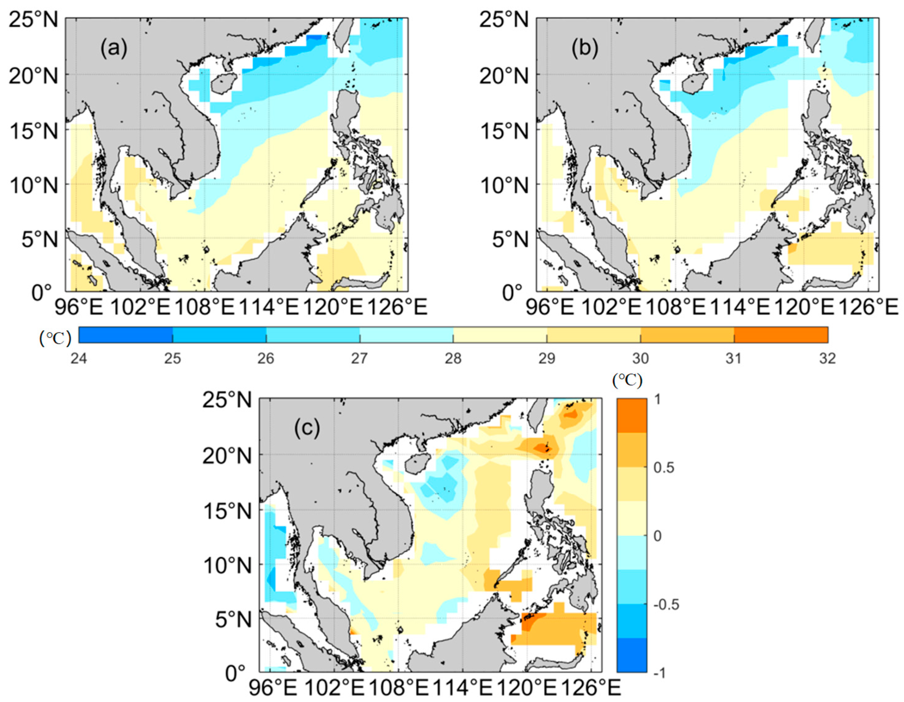
This research assesses the results of the LICOM simulation using the IAP Global Ocean Temperature Grid dataset. The IAP data are the global ocean temperature dataset provided by the Institute of Atmospheric Physics, Chinese Academy of Sciences. This dataset offers high spatial and temporal resolution subsurface temperature data and is widely used in climate and oceanographic research. It provides monthly records from 1940 to the present, with a spatial resolution of 1° × 1°, covering temperature and other physical variables from the sea surface to a depth of 2000 m. Figure 2a shows the annual average SST distribution from IAP. Comparing the difference between the two, it can be seen that although there are some discrepancies between the simulated SST and the IAP data in certain areas, the simulated SST is slightly higher near Borneo Island, while in the Strait of Malacca and nearby waters, the SST is somewhat elevated. However, the overall deviation is small, and the distribution pattern of the LICOM simulated SST is in agreement with the IAP data. This shows that the SST results simulated by the LICOM model are reliable.

4. Results Analysis

4.1. Effect of Wave Mixing on Temperature

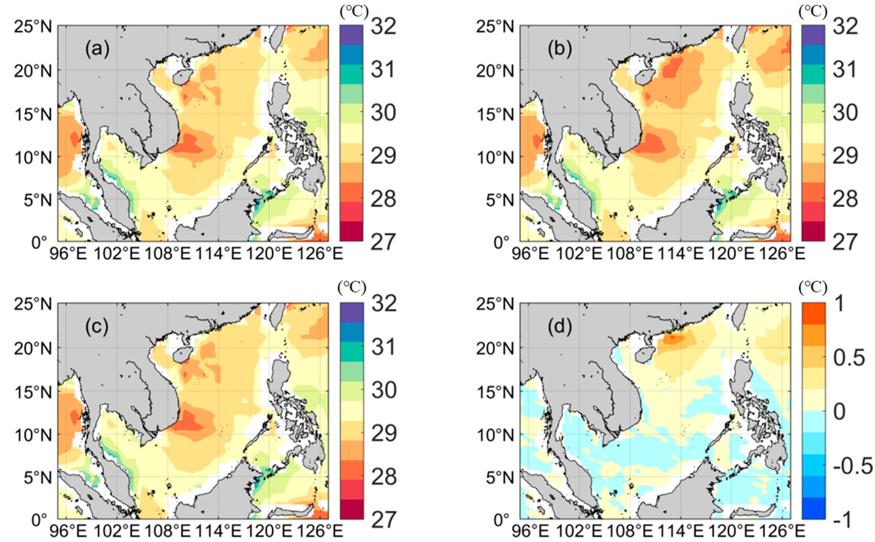
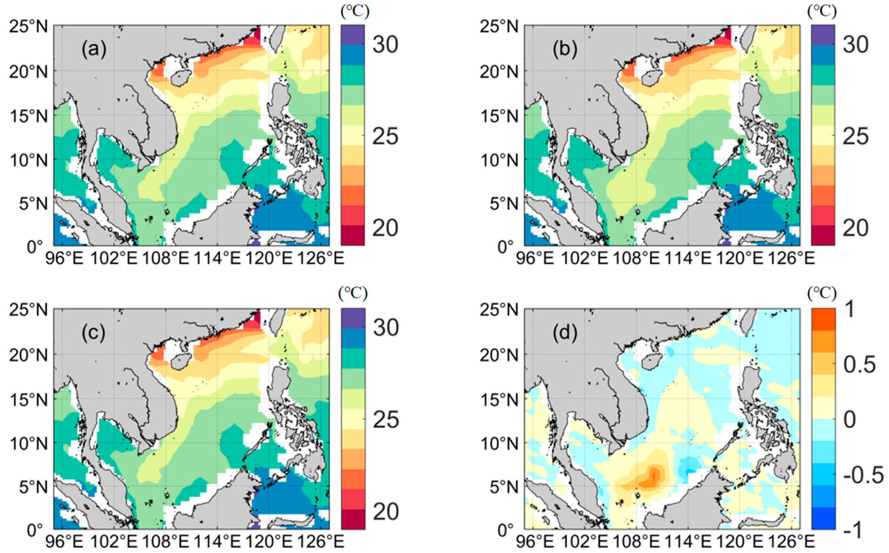
To study the impact of the two parameterization schemes on the model simulation, this study compares and analyzes the simulation results under no-wave conditions, the Bv scheme, and the Pw scheme. The results are shown in Figure 3 and Figure 4. Under no-wave conditions, the SST shows an increasing distribution from south to north. After introducing the Bv parameterization scheme, the SST significantly decreases, with the most noticeable cooling occurring in the southern and central parts of the South China Sea. This indicates that the Bv scheme effectively enhances surface ocean mixing, promoting heat transfer downward. When the Pw scheme is applied, the SST distribution shows minimal changes compared to the no-wave scenario, indicating that the vertical mixing caused by the Pw scheme is relatively weak.
To better analyze the impact of the two parameterization schemes on the SST, a difference analysis was performed. From Figure 3 and Figure 4, it can be seen that in the summer, most areas show a positive difference, primarily focused on the northern and eastern areas and some areas west of Taiwan Island. In these regions, the SST simulated by the Pw scheme is higher, indicating that the cooling effect generated by the mixing process in the Pw scheme is not as significant as that in the Bv scheme. In other words, in the summer, the Bv scheme more effectively enhances vertical mixing through wave-induced mixing, leading to the upwelling of cold water and a significant decrease in SST. Compared to summer, in winter, the area where the SST simulated by the Pw scheme is lower than that of the Bv scheme significantly increases, especially in the central and northeastern areas. This indicates that, compared to summer, the cooling effect of the Pw scheme is more pronounced in winter. Overall, the cooling effect of the Pw scheme on SST is less than that of the Bv scheme, further suggesting that the Bv scheme better strengthens vertical mixing, thereby enhancing the mixing between the surface and deep waters.
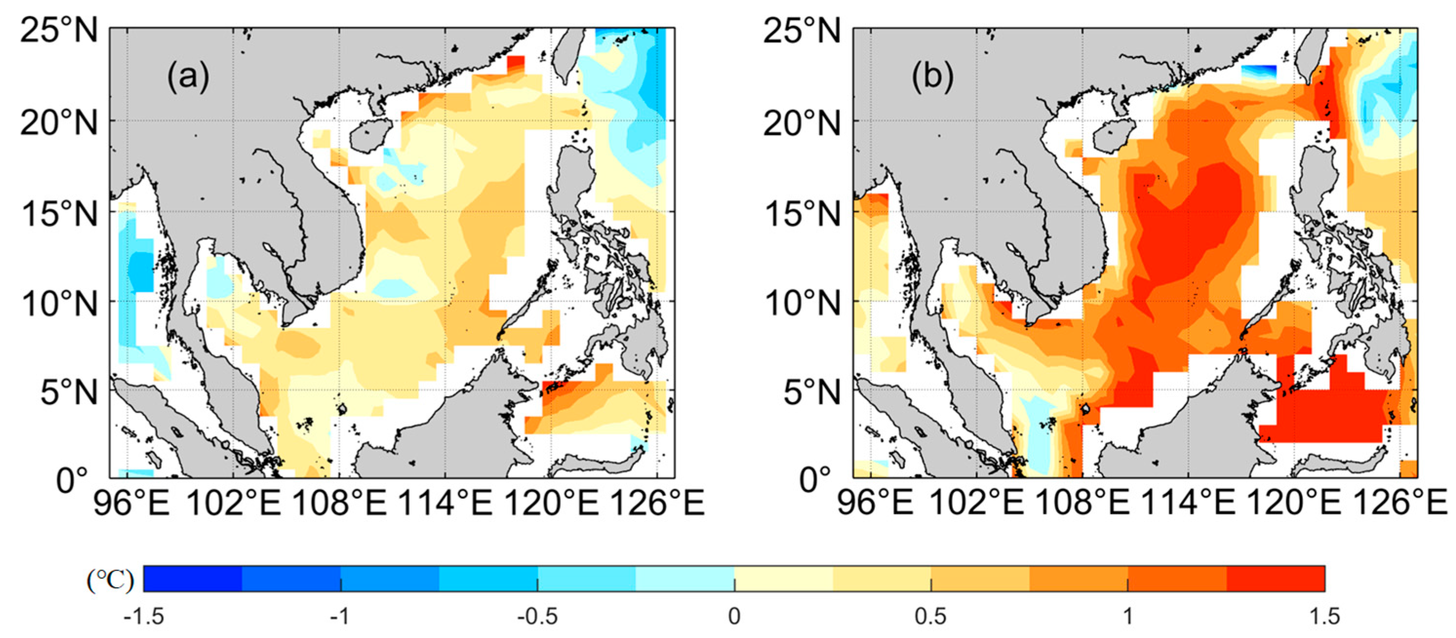
Figure 5a shows the sea surface temperature (SST) differences in summer. Overall, the difference between the two is positive in most sea areas, indicating that the SST simulated by LICOM has a positive bias, with deviations in some regions exceeding 1.5 °C. Figure 5b shows the SST differences in winter. In comparison to summer, the SST difference distribution is more concentrated, mainly showing positive differences over a larger area.
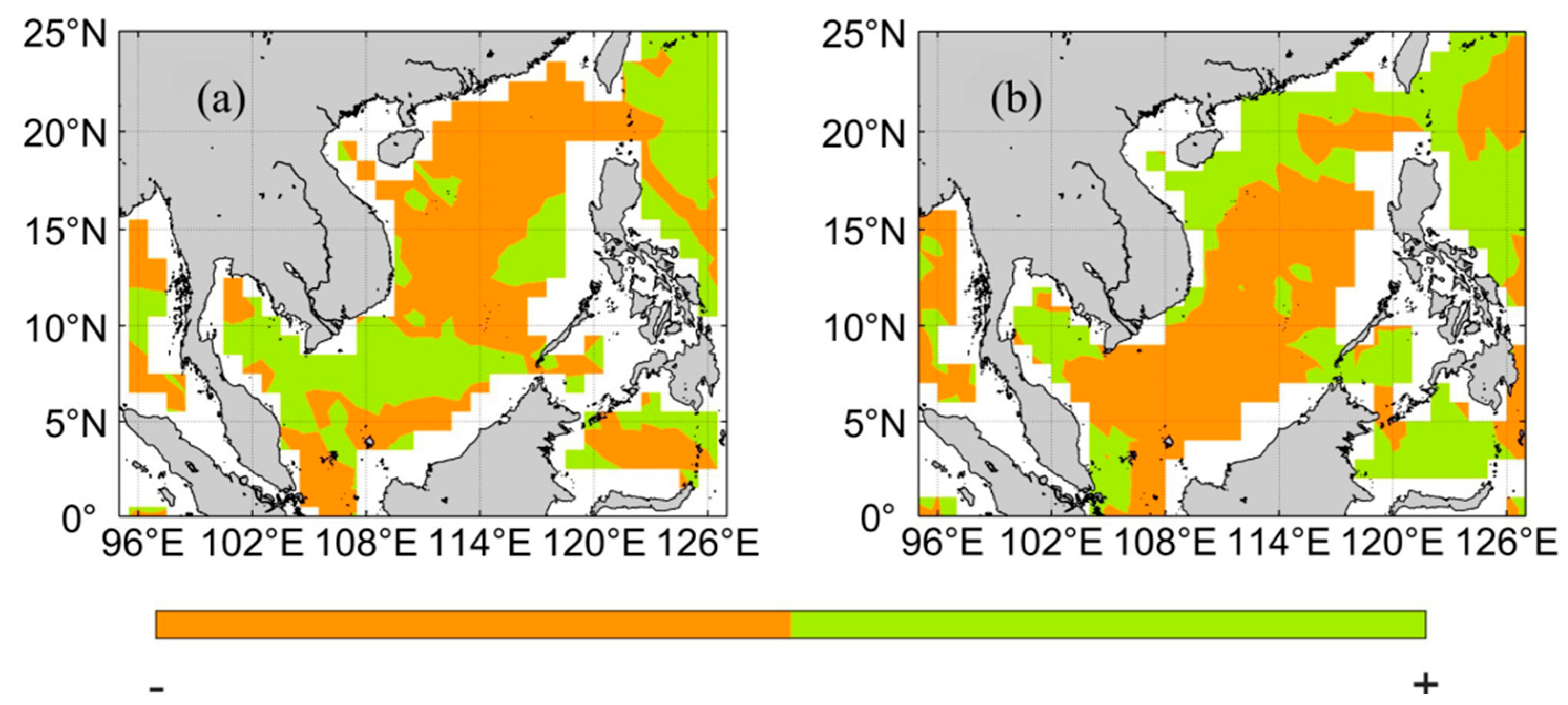
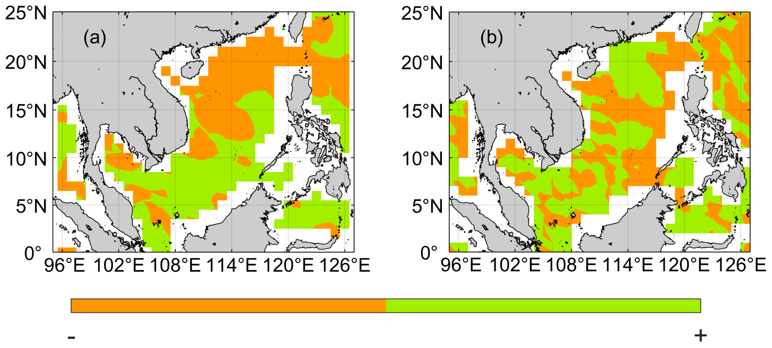
By combining Figure 5 with the changes brought about by waves in Figure 3c and Figure 4c, we can obtain Figure 6 and Figure 7. From these, we can clearly observe how wave mixing alters the simulation biases of the LICOM model. Overall, compared to the Pw scheme, the Bv scheme covers a larger area of improvement in both summer and winter. In the summer, the areas of improvement are primarily focused in the northern region and the waters east of the Philippines. These areas show improvements in the simulation results through the Pw scheme, but the overall improvement is more limited, with significant improvements only in certain local areas. In winter, the areas of improvement for the Pw scheme are relatively scattered, mainly concentrated in regions south of the Indochina Peninsula, around Sumatra, and near the equator. However, the coverage of these improved areas is still quite limited. Particularly near the equator, although some improvement is observed, the overall trend does not cover most areas, and thus the effect is not significant.
In contrast, the Bv scheme performs more prominently in both seasons. In the summer, the areas of improvement for the Bv scheme are more extensive, extending to other parts of the sea, including the Bashi Channel and the central waters. In winter, the improvement effect of the Bv scheme on SST is also superior to that of the Pw scheme, especially in the areas around Sumatra and the southern part of the Indochina Peninsula. Therefore, the overall improvement effect of the Bv scheme is clearly better than that of the Pw scheme.

4.2. Effect of Waves on Vertical Mixing Coefficient

According to the analysis in Section 4.1, there are significant differences between the Bv and Pw parameterization schemes in SST simulations. Specifically, the SST simulated by the Bv scheme is lower than that simulated by the Pw scheme. Although both parameterization schemes can affect the vertical mixing mechanism, they introduce wave mixing in different ways, which leads to differences in their impact on the simulation results. Previous studies have shown that when considering the mixing effects caused by waves, the vertical mixing coefficient in the ocean surface layer increases significantly [8,16]. Therefore, when different parameterization schemes are applied to simulate sea surface temperature, changes in the mixing coefficient become an important factor influencing the simulation results. To further analyze the reasons for the differences in SST simulations between the Bv and Pw schemes, we primarily examine the differences in their vertical mixing coefficients.
When the surface vertical mixing coefficient increases, it leads to increased heat exchange between the surface and subsurface layers, thus affecting the sst. Figure 8 and Figure 9 show the distribution characteristics of the surface mixing coefficient for both parameterization schemes in summer and winter. From the figures, it can be seen that the surface mixing coefficient in the Bv parameterization scheme is generally higher than that in the Pw scheme. This result indicates that the vertical mixing intensity generated by the Bv scheme is significantly stronger than that of the Pw scheme, which explains why the SST is typically lower when the Bv scheme is considered. In contrast, the mixing coefficient in the Pw scheme is lower, and vertical mixing is weaker, leading to relatively higher simulated sea surface temperatures.
To more intuitively reveal the different performances of the Pw and Bv schemes in the mixing mechanism and to analyze the potential impacts on sea surface temperature and the mixed layer structure, we plotted the zonal-averaged vertical mixing rate difference distributions for both schemes in different seasons. Figure 10 shows the zonal-averaged vertical mixing coefficient differences between the Pw and Bv schemes in the upper layer of the South China Sea in summer (a) and winter (b) By analyzing the spatial distribution of the mixing rate differences in the figures, we can more clearly reveal the differences in the mixing mechanisms of the two parameterization schemes and the potential impacts of these differences on sea surface temperature.
In summer, the mixing rate difference in most areas is negative, particularly in the range of 0°~25° N, where there is a significant negative difference between the surface and 50 m. This indicates that the Bv scheme has a higher vertical mixing rate compared to the Pw scheme. Especially in the mid-latitude region of 10° N~20° N, the difference is particularly noticeable. This phenomenon reflects that the Bv parameterization scheme is more effective in enhancing turbulent mixing in the upper ocean during the summer, promoting momentum and heat exchange between the surface and subsurface layers, which leads to relatively lower sea surface temperatures. This is consistent with the previous analysis and further validates the stronger mixing ability of the Bv scheme under summer conditions. In winter, the range of the difference distribution expands further, and the negative value region deepens significantly. Between the latitudes of 10° N and 25° N, the mixing rate difference extends to below 200 m, indicating that the Bv scheme has a more significant impact on mixing deeper water bodies during this season. Compared to the Pw scheme, the Bv scheme not only enhances mixing in the surface layer but also has a deeper impact on deeper waters. Overall, the difference distribution in Figure 10 clearly reveals the systematic differences in mixing rate simulation between the two parameterization schemes. The Bv scheme, by enhancing vertical mixing, effectively extends the vertical influence range of the mixed layer, especially under winter conditions, with a deeper influence and stronger mixing effect, thereby improving the accuracy of the model in simulating upper ocean heat content.
Considering the effect of wave-induced mixing, the enhancement of vertical mixing results in more thorough mixing, which can better transfer heat from the surface layer to the subsurface layer. This inevitably affects the temperature and salinity structure of the entire upper ocean. To further explore the specific impact of mixing intensity differences on the upper ocean thermal structure, this study analyzes the temperature difference distribution between the Pw and Bv schemes in different seasons. Figure 11 shows the impact of wave-induced mixing on the upper ocean temperature in summer (a) and winter (b), with the temperature difference between the Pw scheme and the Bv scheme. By combining the mixing coefficient differences shown in Figure 10, this provides a more comprehensive view of the impact mechanism of the mixing parameterization schemes on the upper thermal structure.
From the summer results, there is a noticeable positive temperature difference near 20° N, primarily within the surface layer to 50 m, indicating that the temperature simulated by the Pw scheme is generally higher than that of the Bv scheme in this region. Combining this with Figure 11a, it can be seen that the mixing rate in the Bv scheme is significantly higher than that in the Pw scheme in this area, which means that stronger vertical mixing transfers heat downward, leading to a reduction in surface temperature. On the other hand, the weaker mixing in the Pw scheme leads to heat accumulation in the upper layer, causing higher temperatures. Additionally, there is also a local temperature difference around 5° N, but the range is smaller.
In winter, the positive temperature difference area is more widespread, mainly located between 5° N and 15° N, from the surface to a depth of 100 m, showing the same trend where the temperature in the Pw scheme is generally higher than in the Bv scheme. This is highly consistent with the winter mixing rate difference distribution shown in Figure 10b. In this latitude range, the Bv scheme generates stronger and deeper vertical mixing, which leads to the upward transport of cold water and downward heat diffusion, thereby lowering the average temperature of the sea surface and upper layers. In contrast, the Pw scheme, due to a smaller mixing rate and a shallower mixing layer, causes heat retention in the upper layers, resulting in relatively higher temperatures. From the vertical structure of the temperature changes, it can be seen that the Bv scheme’s regulation of ocean temperature is not limited to the surface layer. In winter, it even affects the subsurface layer below 200 m, indicating that while enhancing mixing, the Bv scheme also alters the entire upper thermal structure. This reflects that the Bv scheme has a deeper impact and provides a more thorough simulation of the heat transport process.
In conclusion, the temperature differences between the Pw and Bv schemes in Figure 11 reflect the thermodynamic effects of the mixing coefficient differences, further confirming that the Bv parameterization scheme enhances vertical mixing, strengthens the thermal exchange between the surface and subsurface layers, and ultimately lowers the surface temperature, demonstrating a more reasonable thermal structure simulation ability. In contrast, the Pw scheme is relatively insufficient in mixing intensity, leading to heat accumulation in the upper layers. This can be attributed to the fundamental difference in how the two schemes introduce wave-induced mixing. The Pw scheme enhances vertical mixing in an indirect manner by introducing a wave-induced TKE source term into the turbulence closure model. However, this source term primarily acts in the near-surface layer and decays rapidly with depth, resulting in limited energy transfer to deeper waters and thus relatively weak overall mixing intensity. In contrast, the Bv scheme directly increases the vertical diffusion coefficient throughout the upper ocean, effectively strengthening the vertical mixing process and exhibiting a stronger mixing capability with a more direct physical mechanism.

5. Conclusions

This study focuses on the vertical mixing mechanisms induced by waves, with particular emphasis on SST and mixing coefficient as the two key physical quantities. A systematic comparison and evaluation were conducted on the application effects of two non-breaking wave parameterization schemes, Bv and Pw, in numerical simulations of the South China Sea region, aiming to explore the impact of different parameterization schemes on the temperature distribution in the South China Sea.
Although both parameterization schemes enhance vertical mixing in the upper ocean, their mechanisms of action are inconsistent. The Bv scheme directly affects the vertical mixing coefficient, while the Pw scheme alters the vertical mixing coefficient by changing the generation of turbulent kinetic energy [29,32]. As a result, the vertical mixing intensities are different. From the SST simulation results, it is evident that the SST simulated by the Bv scheme is generally lower than that of the Pw scheme in both winter and summer, indicating that the Bv scheme is more effective in transferring surface heat downward, thereby regulating and cooling the sea surface temperature. In contrast, the weaker mixing mechanism of the Pw scheme makes it difficult for heat to be transferred downward, resulting in higher surface temperatures. Regarding improvements in SST simulation, the Bv scheme shows a broader area of improvement in the South China Sea SST.
Further analysis from the perspective of mixing coefficients quantitatively verifies the differences in physical mechanisms between the two schemes. The Bv scheme consistently exhibits higher vertical mixing coefficients in both summer and winter, especially in the typical wind-wave-affected zone between 10° N and 25° N. Compared to the Pw scheme, the Bv scheme demonstrates stronger vertical mixing ability, with the vertical mixing rate maintaining a high level up to a depth of 200 m, reflecting continuous and strong mixing effects. From the vertical structure of temperature changes, it can be observed that the Bv scheme’s regulation of ocean temperature is not limited to the surface layer. In winter, it even affects the subsurface layer below 200 m, indicating that the Bv scheme not only enhances mixing but also alters the entire upper thermal structure. This study only conducted a case analysis, and further expansion of the research scope and time frame is needed in the future.

Author Contributions

Methodology, K.W. and Z.Y.; Resources, Z.Y.; Writing—original draft, Y.J.; Writing—review & editing, R.L.; Supervision, R.L. All authors have read and agreed to the published version of the manuscript.

Funding

We appreciate the funding support from the National Key Research and Development Program of China (Grant No. 2022YFC3105002).

Data Availability Statement

In this study, the IAP datasets available at (http://www.ocean.iap.ac.cn/, accessed on 15 May 2023) were used.

Acknowledgments

We gratefully acknowledge the support of the National Key Scientific and Technological Infrastructure Project, Earth System Numerical Simulation Facility (EarthLab).

Conflicts of Interest

The authors declare no conflict of interest.

References

  1. Rintoul, S.R.; England, M.H. Ekman transport dominates local air-sea fluxes in driving variability of Subantarctic Mode Water. J. Phys. Oceanogr. 2002, 32, 1308–1321. [Google Scholar] [CrossRef]
  2. Sallée, J.B.; Wienders, N.; Speer, K.; Morrow, R. Formation of subantarctic mode water in the southeastern Indian Ocean. Ocean Dyn. 2006, 56, 525–542. [Google Scholar] [CrossRef]
  3. Dong, S.; Sprintall, J.; Gille, S.T.; Talley, L. Southern Ocean mixed-layer depth from Argo float profiles. J. Geophys. Res. Ocean. 2008, 113, C06013. [Google Scholar] [CrossRef]
  4. Sallée, J.B.; Shuckburgh, E.; Bruneau, N.; Meijers, A.J.S.; Bracegirdle, T.J.; Wang, Z. Assessment of Southern Ocean water mass circulation and characteristics in CMIP5 models: Historical bias and forcing response. J. Geophys. Res. Ocean. 2013, 118, 1845–1862. [Google Scholar] [CrossRef]
  5. Stoney, L.; Walsh, K.J.E.; Thomas, S.; Spence, P.; Babanin, A.V. Changes in ocean heat content caused by wave-induced mixing in a high-resolution ocean model. J. Phys. Oceanogr. 2018, 48, 1139–1150. [Google Scholar] [CrossRef]
  6. Eldeberky, Y.; Battjes, J.A. Spectral modeling of wave breaking: Application to Boussinesq equations. J. Geophys. Res. Ocean. 1996, 101, 1253–1264. [Google Scholar] [CrossRef]
  7. Kumar, N.; Voulgaris, G.; Warner, J.C.; Olabarrieta, M. Implementation of the vortex force formalism in the coupled ocean–atmosphere–wave–sediment transport (COAWST) modeling system for inner shelf and surf zone application. Ocean. Model. 2012, 47, 65–95. [Google Scholar] [CrossRef]
  8. Qiao, F.; Yuan, Y.; Yang, Y.; Zheng, Q.; Xia, C.; Ma, J. Wave-induced mixing in the upper ocean: Distribution and application to a global ocean circulation model. Geophys. Res. Lett. 2004, 31, L11303. [Google Scholar] [CrossRef]
  9. Sulisz, W.; Paprota, M. On modeling of wave-induced vertical mixing. Ocean Eng. 2019, 194, 106622. [Google Scholar] [CrossRef]
  10. Thomas, S.; Babanin, A.V.; Walsh, K.J.E.; Stoney, L.; Heil, P. Effect of wave-induced mixing on Antarctic sea ice in a high-resolution ocean model. Ocean Dyn. 2019, 69, 737–746. [Google Scholar] [CrossRef]
  11. Walsh, K.; Govekar, P.; Babanin, A.V.; Ghantous, M.; Spence, P.; Scoccimarro, E. The effect on simulated ocean climate of a parameterization of unbroken wave-induced mixing incorporated into the k-epsilon mixing scheme. J. Adv. Model. Earth Syst. 2017, 9, 735–758. [Google Scholar] [CrossRef]
  12. Babanin, A. On wave-induced turbulence and a wave-mixed upper ocean layer. Geophys. Res. Lett. 2006, 33, L20605. [Google Scholar] [CrossRef]
  13. Jeffreys, H. On turbulence in the ocean. Lond. Edinb. Dublin Philos. Mag. J. Sci. 1920, 39, 578–586. [Google Scholar] [CrossRef]
  14. Buccino, M.; Daliri, M.; Buttarazzi, N.; Del Giudice, G.; Calabrese, M.; Somma, R. Arsenic contamination at the Bagnoli Bay seabed (South Italy) via particle tracking numerical modeling: Pollution patterns from stationary climatic forcings. Chemosphere 2022, 303 Pt 1, 134955. [Google Scholar] [CrossRef] [PubMed]
  15. Martin, P.J. Simulation of the mixed layer at OWS November and Papa with several models. J. Geophys. Res. Ocean. 1985, 90, 903–916. [Google Scholar] [CrossRef]
  16. Hu, H.; Wang, J. Modeling effects of tidal and wave mixing on circulation and thermohaline structures in the Bering Sea: Process studies. J. Geophys. Res. Ocean. 2010, 115, C01006. [Google Scholar] [CrossRef]
  17. Aijaz, S.; Ghantous, M.; Babanin, A.; Ginis, I.; Thomas, B.; Wake, G. Nonbreaking wave-induced mixing in upper ocean during tropical cyclones using coupled hurricane-ocean-wave modeling. J. Geophys. Res. Ocean. 2017, 122, 3939–3963. [Google Scholar] [CrossRef]
  18. He, H.-L.; Song, J.-B.; Bai, Y.-F.; Xu, Y.; Wang, J.-J.; Bi, F. Climate and extrema of ocean waves in the East China Sea. Sci. China Earth Sci. 2018, 61, 980–994. [Google Scholar] [CrossRef]
  19. Tolman, H.L. User Manual and System Documentation of WAVEWATCH III Version 3.14; NOAA/NWS/NCEP/MMAB Technical Note 276; National Oceanic and Atmospheric Administration: Silver Spring, MD, USA, 2009.
  20. Komen, G.J.; Cavaleri, L.; Donelan, M.; Hasselmann, K.; Hasselmann, S.; Janssen, P.A.E.M. Dynamics and Modelling of Ocean Waves; Cambridge University Press: Cambridge, UK, 1994. [Google Scholar] [CrossRef]
  21. Ardhuin, F.; Rogers, E.; Babanin, A.V.; Filipot, J.-F.; Magne, R.; Roland, A.; van der Westhuysen, A.; Queffeulou, P.; Lefevre, J.-M.; Aouf, L.; et al. Semi-empirical dissipation source functions for ocean waves. Part I: Definition, calibration and validation. J. Phys. Oceanogr. 2010, 40, 1917–1941. [Google Scholar] [CrossRef]
  22. Atlas, R.; Hoffman, R.N.; Ardizzone, J.; Leidner, S.M.; Jusem, J.C.; Smith, D.K.; Gombos, D. A cross-calibrated, multi-platform (CCMP) ocean surface wind product for meteorological and oceanographic applications. Bull. Am. Meteorol. Soc. 2011, 92, 157–174. [Google Scholar] [CrossRef]
  23. Liu, H.; Lin, P.; Yu, Y.; Zhang, X. The baseline evaluation of LASG/IAP climate system ocean model (LICOM) version 2. Acta Meteorol. Sin. 2012, 26, 318–329. [Google Scholar] [CrossRef]
  24. Liu, H.; Lin, P.; Zheng, W.; Luan, Y.; Ma, J.; Ding, M.; Mo, H.; Wan, L.; Ling, T. A global eddy-resolving ocean forecast system in China—LICOM Forecast System (LFS). J. Oper. Oceanogr. 2021, 16, 15–27. [Google Scholar] [CrossRef]
  25. Canuto, V.M.; Howard, A.; Cheng, Y.; Dubovikov, M.S. Ocean turbulence. Part I: One-point closure model-momentum and heat vertical diffusivities. J. Phys. Oceanogr. 2001, 31, 1413–1426. [Google Scholar] [CrossRef]
  26. Canuto, V.M.; Dubovikov, M.S.; Howard, A.M.; Cheng, Y. Ocean turbulence. Part II: Vertical diffusivities of momentum, heat, salt, mass, and passive scalars. J. Phys. Oceanogr. 2002, 32, 240–264. [Google Scholar] [CrossRef]
  27. Babanin, A. Breaking and Dissipation of Ocean Surface Waves; Cambridge University Press: Cambridge, UK, 2011. [Google Scholar]
  28. Babanin, A.V.; Haus, B.K. On the existence of water turbulence induced by nonbreaking surface waves. J. Phys. Oceanogr. 2009, 39, 2675–2679. [Google Scholar] [CrossRef]
  29. Ghantous, M.; Babanin, A.V. One-dimensional modelling of upper ocean mixing by turbulence due to wave orbital motion. Nonlinear Process. Geophys. 2014, 21, 325–338. [Google Scholar] [CrossRef]
  30. Young, I.; Babanin, A.V.; Zieger, S. The decay rate of ocean swell observed by altimeter. J. Phys. Oceanogr. 2013, 43, 2322–2333. [Google Scholar] [CrossRef]
  31. Qiao, F.L.; Yuan, Y.L.; Ezer, T.; Xia, C.S.; Ma, J. A three-dimensional surface wave–ocean circulation coupled model and its initial testing. Ocean. Dyn. 2010, 60, 1339–1355. [Google Scholar] [CrossRef]
  32. Li, Y.; Qiao, F.; Yin, X.; Shu, Q.; Ma, H. The improvement of the one-dimensional Mellor–Yamada and K-profile parameterization turbulence schemes with the non-breaking surface wave-induced vertical mixing. Acta Oceanol. Sin. 2013, 32, 62–73. [Google Scholar] [CrossRef]
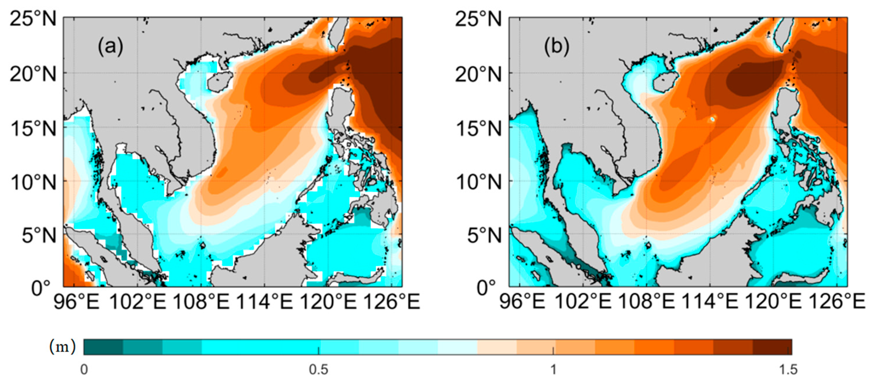
Figure 1. Annual SWH (m): (a) ERA5 (b) WW3.
Jmse 13 01548 g001
Figure 2. Simulated annual mean SST distribution characteristics: (a) IAP (b) LICOM (c) Distribution of interpolated values (LICOM—IAP).
Jmse 13 01548 g002
Figure 3. Summer simulated SST (°C) difference distribution: (a) No-wave prediction result (b) Bv scheme prediction result (c) Pw scheme prediction result (d) Difference between Pw and Bv schemes (Pw-Bv).
Jmse 13 01548 g003
Figure 4. Winter simulated SST (°C) difference distribution: (a) No-wave prediction result (b) Bv scheme prediction result (c) Pw scheme prediction result (d) Difference between Pw and Bv schemes (Pw-Bv).
Jmse 13 01548 g004
Figure 5. SST Difference Distribution (LICOM-IAP) (a) Summer (b) Winter.
Jmse 13 01548 g005
Figure 6. SST Simulation Improvement Caused by Bv: (a) Summer (b) Winter (Red represents improvement, while green signifies deterioration.).
Jmse 13 01548 g006
Figure 7. SST Simulation Improvement Caused by Pw: (a) Summer (b) Winter (Red represents improvement, while green signifies deterioration).
Jmse 13 01548 g007
Figure 8. Summer surface mixing coefficient (cm2/s): (a) Pw (b) Bv.
Jmse 13 01548 g008
Figure 9. Winter surface mixing coefficient (cm2/s): (a) Pw (b) Bv.
Jmse 13 01548 g009
Figure 10. Zonal-averaged vertical mixing coefficient (Pw-Bv) (cm2/s): (a) Summer (b) Winter.
Jmse 13 01548 g010
Figure 11. The difference in Zonal-averaged upper ocean temperature (Pw-Bv) (°C): (a) Summer (b) Winter.
Jmse 13 01548 g011
Disclaimer/Publisher’s Note: The statements, opinions and data contained in all publications are solely those of the individual author(s) and contributor(s) and not of MDPI and/or the editor(s). MDPI and/or the editor(s) disclaim responsibility for any injury to people or property resulting from any ideas, methods, instructions or products referred to in the content.