A Systematic Evaluation of the New European Wind Atlas and the Copernicus European Regional Reanalysis Wind Datasets in the Mediterranean Sea

Abstract

The Copernicus European Regional Reanalysis (CERRA) was released in August 2022, providing a continental atmospheric reanalysis, and, in addition, the New European Wind Atlas (NEWA) is a recently released hindcast product that can be used to create a high temporal and spatial resolution wind resource atlas of Europe. In order to demonstrate the suitability of the NEWA and CERRA wind datasets for offshore wind energy applications, the accuracy of these datasets was assessed for the Mediterranean Sea, a basin with a high potential for the development of offshore wind projects. Long-term in situ measurements from 13 offshore locations along the basin were used in order to assess the performance of the CERRA and NEWA wind speed datasets in the hourly and seasonal time scales by using a variety of different evaluation tools. The results revealed that the CERRA dataset outperforms NEWA and is a reliable source for offshore wind energy assessment studies in the examined areas, although special attention should be paid to extreme value analysis of the wind speed.

1. Introduction

Accurate and high-resolution wind speed data are essential for a variety of applications that depend on the reliable estimation of the atmospheric state. Taking into consideration the scarcity of wind speed data over sea areas, where the deployment of site-specific instruments (e.g., fixed or floating mast, buoy, LiDAR) is more difficult and cost-intensive than onshore, the use of reanalysis products has gained a lot of attention in regional wind energy studies as e.g., in [1], where the authors used the SKIRON hindcast product, in [2,3] where ERA5 reanalysis product has been used, and relevant analyses even at the global scale as e.g., in [4], using ERA-Interim reanalysis product, and [5] using the Cross-Calibrated Multi-Platform (CCMP) wind field data. Other related methods aiming at the same outcomes are based on satellite data as e.g., in [6,7,8,9], and gridded products constructed by interpolating observational data [10,11]. Some of the advantages of the reanalysis data include the long-term time series that allow the estimation of interannual variability, the spatial coverage that extends to remote and offshore locations and their availability and accessibility; however, their coarse spatial resolution poorly captures complicated topographical features, leading to inadequate representation of local climatic conditions [12].

Wind reanalysis datasets are a combination of atmospheric model and wind observational data spanning back some decades using an assimilation scheme. Specifically, over a long-time span, these reanalysis datasets can provide wind speed estimates for every grid point of the model domain at each assimilation time and level. The provision of wind information in extended areas at multiple vertical atmospheric levels [13,14] is a preliminary tool for the better understanding of the wind climate evolution and the prevailing wind speed regional patterns.

In order to verify the suitability of hindcast data for a particular region, the most credible method is to compare them with long-term in situ wind measurements (of several years length), a data source of high accuracy [15], in order to assess intraday, seasonal, mean annual and interannual variability. It should be emphasized that when reanalysis datasets are compared with other model products, this may lead to less robust and safe conclusions regarding the performance of the dataset under evaluation. Several studies that deal with the comparison of reanalysis datasets with measured data have used evaluation and correlation metrics as well as probability distributions, e.g., [16,17].

The Copernicus European Regional Reanalysis (CERRA) was released in August 2022, providing a continental reanalysis with very high spatial resolution [18]. The main predecessor of CERRA is Uncertainties in Ensembles of Regional Reanalysis (UERRA), available for download until 2019. ERA-lnterim [19] is the global reanalysis used as the lateral boundary of the UERRA regional reanalysis, while ERA5 [20], produced by the European Centre for Medium-Range Weather Forecasts (ECMWF) with global coverage, is used as the lateral boundary for CERRA (https://confluence.ecmwf.int/display/CKB/Copernicus+European+Regional+ReAnalysis+%28CERRA%29%3A+product+user+guide (accessed on 25 March 2025)).

The CERRA dataset has been validated in terms of on-shore air temperature, relative humidity, 10 m wind speed and global solar radiation in Greece by using up to 11-year-long ground-based observations and has been also compared to the ERA5-Land dataset [21]. The results of that study revealed that the CERRA dataset significantly outperformed the ERA5-Land reanalysis data with respect to the measured meteorological variables in the North (NA) and South Aegean (SA). Specifically, the seasonal root mean squared ($RMSE$) values of CERRA and ERA5 wind speed at 10 m are summarized in

Table 1. RMSE values (in m/s) of CERRA and NEWA wind speed data at 10 m compared to wind measurements (according to [21]).

Season	North Aegean		South Aegean
	CERRA	ERA5	CERRA	ERA5
Winter	1.65	2.88	1.21	1.01
Spring	1.34	2.42	1.69	2.29
Summer	1.13	2.79	1.65	2.25
Autumn	1.37	2.62	1.70	2.43

.

Hadjipetrou and Kyriakidis [22], reported that CERRA exhibited the strongest agreement with in situ onshore wind speed measurements in the eastern Mediterranean basin. Rouholahnejad et al. [23] comparatively assessed ERA5, CERRA and WRF based on measured wind data in the North Sea. They concluded that CERRA demonstrated great accuracy in wind speed distribution with low errors in both extreme values (95th percentile) and mean bias. Pelosi [24] evaluated different meteorological variables from CERRA (including wind speed at 10 m), with interpolated ground-based data and found that CERRA wind speed performance showed the least accuracy in complex terrain areas of Sicily Isl. Jourdier et al. [25] comparatively evaluated the performance of CERRA wind speed at 100 m with ERA5 and COSMO-REA6. CERRA exhibited larger differences in relation to ERA5, with higher wind speeds over most of Europe, while in relation to COSMO-REA6, the differences were smaller. Finally, Spangehl et al. [26] evaluated the performance of CERRA near-surface wind speed based on satellite observations in the North Sea and concluded that it exhibits a systematic overestimation.

The New European Wind Atlas (NEWA) [27] is a recent initiative to create a high resolution wind resource atlas of Europe 1. One of the most important components of the initiative was conducting extensive sensitivity studies and production runs using the Weather Research and Forecasting (WRF) mesoscale model [28]. The objective was to establish a well-informed model setup, based on scientific evaluation, for the production of a mesoscale wind atlas. The NEWA wind atlas has been evaluated in various publications. For example, Murcia et al. [29], based on onshore wind measurements from 32 tall meteorological masts in Europe, examined three different mesoscale reanalysis models including NEWA and ERA5 and concluded that NEWA performs better than ERA5, although it overestimates wind speed. Kalverla et al. [30] compared the performance of ERA-5, Dutch Offshore Wind Atlas (DOWA), and NEWA wind reanalyses using measurements from the Met Mast IJmuiden in the North Sea. The results showed that NEWA accurately predicted near surface wind speeds, but underestimated wind shear. As mentioned before, Hadjipetrou and Kyriakidis [22] evaluated five high resolution wind speed reanalyses, CERRA and NEWA included, with coastal (on shore) in situ measurements from five meteorological stations in the eastern Mediterranean during the 2009–2018 period. Among the examined five datasets, CERRA and NEWA exhibited the highest alignment with measured wind speeds; although NEWA overestimated mean values, it captured extremes effectively. Meyer et al. [31] compared ERA5 and NEWA datasets for offshore wind resource assessment across multiple North and Central European offshore areas, including the Irish Sea, Baltic Sea, North Sea and English Channel. In their analysis, NEWA exhibited increased accuracy regarding mean wind speed values and better overall wind speed variability assessment due to its higher temporal resolution, but both datasets underestimated extreme wind speeds. That study also examined the effectiveness of the spectral correction method in 50-year return wind speed predictions, finding it adequate for certain sites, yet inadequate for others, something that highlights the need for more localised validation approaches. Araveti et al. [32] examined four different reanalysis products, including ERA5 and NEWA, at four onshore locations in Ireland. The authors concluded that ERA5 outperforms the other products, while they also emphasized that NEWA exhibited the poorest performance combined with an anomaly at 100 m and 110 m levels above ground wind speed. Jourdier [33] compared five different wind datasets (ERA5 and NEWA included) using wind measurements from seven onshore meteorological masts and one LIDAR in France. The author concluded that ERA5 performed very well, although underestimating wind speeds in mountainous areas, while NEWA presented large biases and overestimated wind speeds, especially at night.

The objective of the present study is to assess and compare the accuracy and performance of CERRA and NEWA wind datasets for the Mediterranean Sea in order to confirm that they can used for preliminary offshore wind energy applications. The economic viability of a wind energy project and other important factors during the design of an offshore wind farm (e.g., wake effects) are highly dependent on the wind regime, especially wind speed, of the location of interest. Thus, the CERRA and NEWA datasets were evaluated for various aspects encountered in wind energy studies. Specifically, in situ measurements from 13 buoy locations were used along the Mediterranean Sea in order to assess the performance of the CERRA and NEWA wind speed data at the annual and seasonal time scales through a variety of evaluation metrics, namely the root mean squared error, bias, Pearson correlation coefficient, mean absolute error, scatter index, and the Hanna–Heinhold indicator. The CERRA and NEWA datasets have been collocated at the spatial and temporal scale with the buoys, using an inverse distance weighting interpolation.

The wind data sources and the methodology, including the collocation procedure for reanalysis and the in situ data and the evaluation metrics used in this work are described in Section 2. The numerical results of the evaluation of the CERRA and NEWA wind datasets at two different temporal scales in order to assess their performance quality are presented in Section 3. Finally, in Section 4, the main findings and remarks of this study are summarized.

2. Data and Methodology

2.1. Copernicus European Regional Reanalysis (CERRA)

CERRA was initially developed through a project led by the Swedish Meteorological and Hydrological Institute (SMHI) in collaboration with Météo-France and the Norwegian Meteorological Institute (MET Norway). The CERRA reanalysis system is based on the “Hirlam Aladin Research Mesoscale Operational NWP In Europe” (HARMONIE) numerical weather prediction (NWP) system with ALADIN (Aire Limitée Adaptation dynamique Développement InterNational) physics and dynamics [18,34]. It improves upon previous European reanalysis databases by adding new advances in modelling and data assimilation techniques. CERRA incorporates a broad range of observational data derived from surface stations, ships, aircraft, drifting buoys and radiosonde/balloon reports to constrain the model state.

For the surface and upper-air analyses, it uses an optimal interpolation assimilation scheme and a three-dimensional variational (3D-VAR) data assimilation scheme, respectively, with a horizontal resolution of 5.5 km and a vertical one of 106 levels. The ERA5 reanalysis is used as input for the lateral boundary conditions of CERRA. Apart from the high spatial resolution, additional improvements of the CERRA system include:

• The assimilation of additional observations, available from the observing system, throughout the reanalysis period in order to represent more accurately the atmospheric conditions. These observations are obtained from ECMWF’s Meteorological Archival and Retrieval System (MARS) and the European Centre File Storage system (ECFS), and include conventional (e.g., synoptic surface observations, drifting buoys, ships) and other observations, such as scatterometer and radiance observations [35].
• The Ensemble Data Assimilation (EDA) system coupled with the deterministic CERRA system to regularly estimate the background error covariance matrix (B-Matrix) with flow-dependency updates [36] to sufficiently represent errors when changes in the weather regime are detected.

The model domain spans in terms of the north-to-south axis from northern Africa beyond the northern tip of Scandinavia and in terms of the west-to-east axis from the Atlantic Ocean up to the Ural Mountains. The model grid is Lambert conformal conic comprising 1069 × 1069 grid points. CERRA covers a period of 38 years (1984–2021), which will be constantly updated, and assimilates eight times per day (i.e., 3 h temporal resolution). The dataset can be obtained through the Copernicus Climate Data Store (https://cds.climate.copernicus.eu/#!/home (accessed on 10 January 2025)).

2.2. New European Wind Atlas (NEWA)

The New European Wind Atlas (NEWA) [37,38], aims to provide thorough, accurate, and sound information on the European wind resource, necessary for commercial evaluations of wind farms. The ERA-Interim reanalysis data (with 0.75° × 0.75° spatial resolution) were used by the NEWA project to provide the dynamic forcing, initial and boundary conditions for the WRF model simulations [38], while observational data from meteorological masts across Europe were used to validate the numerical simulations.

Regarding the properties of NEWA model data, sensitivity tests [39] were initially conducted using WRF version 3.6.1, while later tests employed version 3.8.1. The initial sensitivity experiments were performed in five distinguished 3 km × 3 km domains in Europe, as this resolution seems to be the standard [40], and used three nested grids with horizontal resolutions of 27 km, 9 km, and 3 km, with 61 grid points in each direction for the outer nest. In addition, the model configuration used 61 vertical levels and 30 min time resolution, therefore making it an adequate source of data for this particular study. See also [27], where a detailed sensitivity analysis and extended evaluation procedures are described in order to select the optimal setup of the WRF simulations. An innovative aspect of NEWA was the use of multi-parameter ensemble simulations in order to address uncertainties in wind resource estimation. The ensembles consisted of WRF runs with different configurations, physical parameterization schemes, initialization, and boundary conditions. The extensive sensitivity studies conducted within the NEWA project helped to identify a well-founded WRF model configuration for the mesoscale wind atlas production runs. The final setup was used to offer a complete wind resource dataset of Europe’s wind resource, supplied with insights from the ensemble simulations associated with uncertainty in wind resource assessment. The production and evaluation of the NEWA wind atlas is analytically described in [41]. The time series length of NEWA is 30 years (extending from 1989 to 2018). However, only the last 10 years (2009–2018) are currently available. NEWA wind data can be accessed and downloaded from https://map.neweuropeanwindatlas.eu/ (accessed on 10 January 2025).

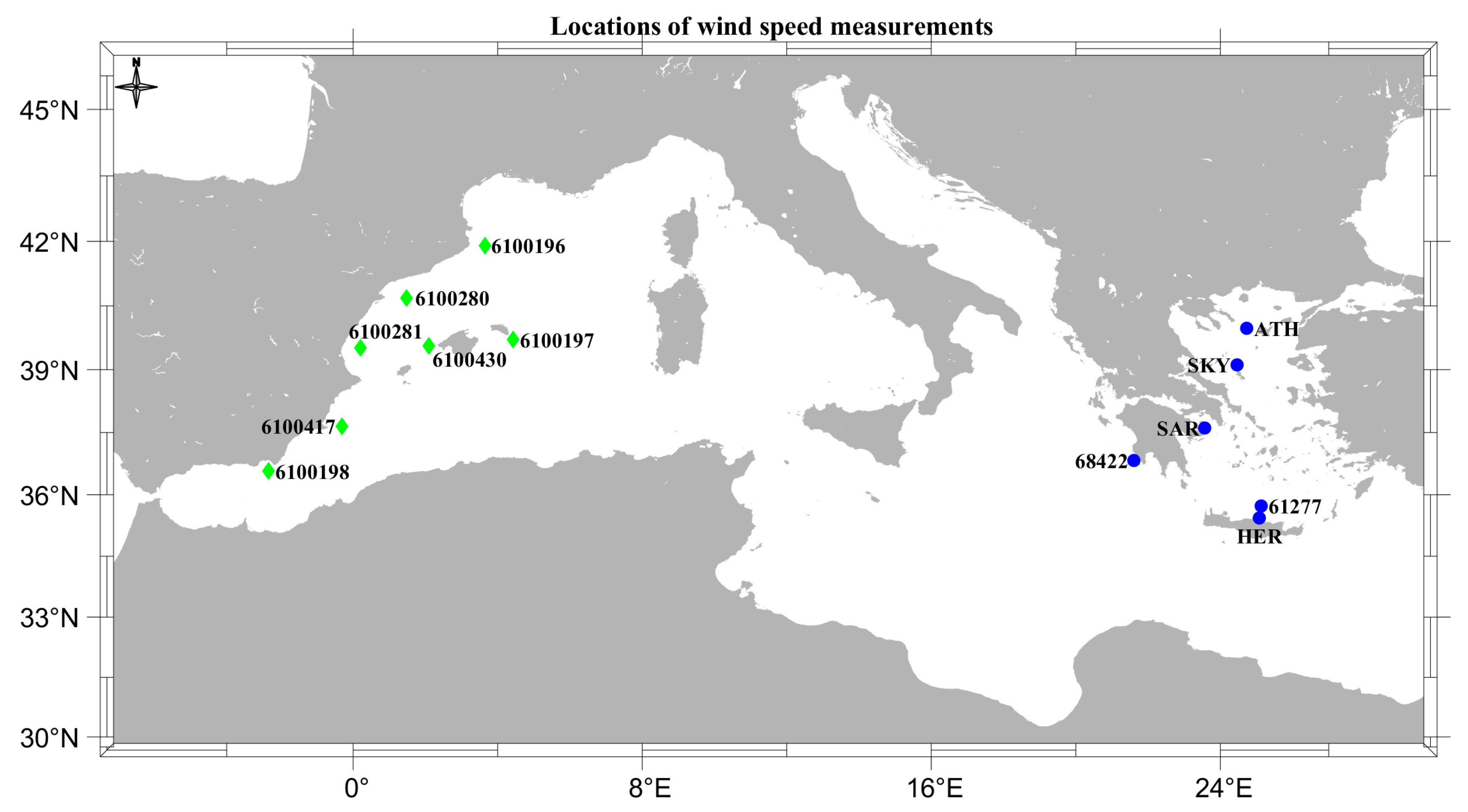
2.3. In Situ Wind Measurements

Long-term measured wind speed data were obtained from the Copernicus Marine Service-ocean in situ data (https://marineinsitu.eu/dashboard/ (accessed on 10 January 2025)). The In Situ Thematic Assembly Centre (TAC) is a component of the Copernicus Marine Service that provides access to a range of in situ met-ocean and environmental measured data (e.g., wind, waves, currents, etc.) derived from a variety of measuring platforms (e.g., radars, moorings, profilers, gliders, drifters, etc.). For wind data, the main source of information is moorings, i.e., oceanographic buoys equipped with wind measurement devices. Most of the available buoys are located in the western and central–eastern Mediterranean, while for the central and western Mediterranean, no buoys are available. The Greek buoys are part of the POSEIDON network [42] that started operating in 1999 under the responsibility of the Hellenic Centre for Marine Research (HCMR). The western Mediterranean buoys operate under the responsibility of the Spanish Operational Marine Climate Monitoring and Forecasting System-Spanish Port Authority (Puertos del Estado) and Météo-France / Ifremer. In order to enrich the available information, four additional buoys were considered for the Greek Seas, bringing the total number of buoys to 13 2.

The buoy data consist of wind speed time series, which cover large time periods. The wind measurements have different recording intervals ranging from 1 to 3 h. The locations of the 13 examined buoys along with their code numbers that were used in this work, with the corresponding measurement periods and the overlapping time periods with CERRA and NEWA wind data, are listed below in

Table 2. Buoy locations, corresponding measurement period and overlapping time periods with CERRA and NEWA wind speed data.

Buoy Code	Latitude (o)	Longitude (o)	Measurement Period	Overlapping Time Periods
				CERRA	NEWA
6100196	41.9000	3.6500	27 March 2001–18 November 2024	2001–2020	2009–2018
6100197	39.7100	4.4200	29 April 1993–30 November 2024	1993–2020	2009–2018
6100198	36.5700	–2.3400	27 March 1998–30 November 2024	1998–2020	2009–2018
6100280	40.6900	1.4700	20 August 2004–30 November 2024	2004–2020	2009–2018
6100281	39.5100	0.2000	15 September 2005–13 November 2024	2005–2020	2009–2018
6100417	37.6500	–0.3100	18 July 2006–30 November 2024	2006–2020	2009–2018
6100430	39.5600	2.0900	29 November 2006–30 November 2024	2006–2020	2009–2018
61277	35.7263	25.1307	28 May 2007–21 November 2024	2007–2020	2009–2018
68422	36.8288	21.6068	9 November 2007–1 April 2023	2007–2020	2009–2018
ATH	39.9750	24.7294	25 May 2000–26 November 2022	2000–2020	2009–2018
HER	35.4342	25.0792	15 July 2016–29 October 2024	2016–2020	2016–2018
SAR	37.6099	23.5669	27 August 2007–1 August 2019	2007–2019	2009–2018
SKY	39.1130	24.4640	28 August 2007–18 July 2012	2000–2012	2009–2012

; see also Figure 1. All the wind measurements have been performed at the reference height of 3 m above sea level (asl). The corresponding sample sizes of the collocated buoy-model data are shown in

Table 3. Statistical parameters of collocated in situ measurements and CERRA.

#	$\mathit{N}$	${\mathit{m}}_{{\mathit{U}}_{\mathit{B}}}$ (m/s)	${\mathit{m}}_{{\mathit{U}}_{\mathit{C}}}$ (m/s)	${\mathit{m}\mathit{e}\mathit{d}}_{{\mathit{U}}_{\mathit{B}}}$ (m/s)	${\mathit{m}\mathit{e}\mathit{d}}_{{\mathit{U}}_{\mathit{C}}}$ (m/s)	${\mathit{C}\mathit{V}}_{{\mathit{U}}_{\mathit{B}}}$ (%)	${\mathit{C}\mathit{V}}_{{\mathit{U}}_{\mathit{C}}}$ (%)	${\mathit{m}\mathit{a}\mathit{x}}_{{\mathit{U}}_{\mathit{B}}}$ (m/s)	${\mathit{m}\mathit{a}\mathit{x}}_{{\mathit{U}}_{\mathit{C}}}$ (m/s)	${\mathit{U}}_{\mathit{B},95}$ (m/s)	${\mathit{U}}_{\mathit{C},95}$ (m/s)	${\mathit{U}}_{\mathit{B},99}$ (m/s)	${\mathit{U}}_{\mathit{C},99}$ (m/s)
6100196	33782	6.91	7.69	5.70	6.46	70.0	62.7	27.9	28.8	16.5	17.0	19.9	20.4
6100197	50912	6.04	6.05	5.47	5.44	59.8	56.0	24.5	22.7	13.1	12.6	16.3	15.8
6100198	48341	6.03	6.56	5.47	6.14	62.1	59.2	22.2	24.3	12.8	13.4	15.9	16.7
6100280	43592	5.04	5.40	4.36	4.62	67.0	62.7	21.4	22.5	11.7	12.1	14.9	15.2
6100281	38111	5.02	5.09	4.36	4.36	64.2	61.7	21.1	20.6	11.2	11.3	14.1	13.8
6100417	37063	5.41	5.73	4.97	5.31	57.4	53.6	19.9	19.7	11.2	11.5	13.8	14.0
6100430	36647	5.30	5.33	4.70	4.69	61.7	60.1	23.0	22.1	11.7	11.6	14.7	14.9
61277	24523	6.14	5.99	5.89	5.72	50.9	47.9	20.9	19.1	11.8	11.2	14.6	13.8
68422	24375	5.36	5.49	4.97	5.12	58.1	55.6	20.7	20.6	11.2	11.1	14.1	14.3
ATH	44736	5.30	5.94	4.54	5.18	69.5	61.7	24.5	21.9	12.4	13.0	16.2	16.1
HER	8734	6.12	5.33	6.09	5.39	49.3	50.4	20.1	18.2	10.9	9.5	14.1	12.9
SAR	21407	5.15	4.90	4.81	4.62	60.1	56.5	19.3	19.0	10.7	9.7	13.1	12.5
SKY	10676	5.63	6.26	5.10	5.87	62.3	55.5	20.9	21.3	12.1	12.6	15.2	15.6

and

Table 4. Statistical parameters of collocated in situ measurements and NEWA.

#	$\mathit{N}$	${\mathit{m}}_{{\mathit{U}}_{\mathit{B}}}$ (m/s)	${\mathit{m}}_{{\mathit{U}}_{\mathit{N}}}$ (m/s)	${\mathit{m}\mathit{e}\mathit{d}}_{{\mathit{U}}_{\mathit{B}}}$ (m/s)	${\mathit{m}\mathit{e}\mathit{d}}_{{\mathit{U}}_{\mathit{N}}}$ (m/s)	${\mathit{C}\mathit{V}}_{{\mathit{U}}_{\mathit{B}}}$ (%)	${\mathit{C}\mathit{V}}_{{\mathit{U}}_{\mathit{N}}}$ (%)	${\mathit{m}\mathit{a}\mathit{x}}_{{\mathit{U}}_{\mathit{B}}}$ (m/s)	${\mathit{m}\mathit{a}\mathit{x}}_{{\mathit{U}}_{\mathit{N}}}$ (m/s)	${\mathit{U}}_{\mathit{B},95}$ (m/s)	${\mathit{U}}_{\mathit{N},95}$ (m/s)	${\mathit{U}}_{\mathit{B},99}$ (m/s)	${\mathit{U}}_{\mathit{N},99}$ (m/s)
6100196	76427	6.94	7.65	5.70	6.43	69.6	64.6	26.7	27.4	16.4	17.7	19.9	21.8
6100197	98096	6.08	6.51	5.47	6.03	59.8	55.1	24.8	25.3	13.1	13.3	16.4	16.9
6100198	89363	6.11	7.36	5.70	7.22	61.6	54.5	23.0	25.1	12.8	14.2	15.9	17.6
6100280	113775	5.02	5.53	4.36	4.73	66.9	63.5	21.9	24.7	11.7	12.8	14.7	16.6
6100281	99809	5.02	5.26	4.36	4.53	63.8	62.4	21.1	24.3	11.2	11.7	13.9	15.1
6100417	92900	5.40	6.15	4.97	5.86	57.9	52.1	19.9	22.4	11.2	11.9	13.8	14.8
6100430	94425	5.32	5.81	4.91	5.28	61.4	58.5	24.8	22.4	11.7	12.3	14.7	15.8
1277	20009	6.05	6.62	5.84	6.50	51.4	47.4	20.9	21.6	11.8	12.3	14.4	15.2
8422	22851	5.37	6.22	4.97	6.02	58.4	53.3	20.7	25.6	11.2	12.1	14.1	15.4
ATH	31509	5.50	5.92	4.71	5.31	65.7	60.6	22.5	23.7	12.6	12.7	16.0	16.0
HER	6102	6.07	6.69	5.96	6.86	51.1	49.7	20.1	24.0	11.2	12.1	14.4	15.3
SAR	21048	5.15	5.34	4.79	4.94	60.3	59.5	19.3	21.4	10.7	11.2	13.1	14.4
SKY	10455	5.62	6.35	5.09	6.01	62.4	55.9	20.9	22.4	12.1	12.8	15.2	16.4

.

The in situ data provided in https://marineinsitu.eu/dashboard/ (accessed on 10 January 2025) have undergone quality control (QC) by the providing organizations and quality flags have been assigned to each value of the examined parameters. For example, the quality flags and their interpretation for wind speed are 0 (no QC was performed), 1 (good data), 2 (probably good data), 3 (bad data that are potentially correctable), 4 (bad data), 5 (value changed), 6 (value below detection /quantification), 7 (nominal value), 8 (interpolated value), and 9 (missing value); see [43], Annex A, Table 1. In order to avoid unnecessary uncertainties, only data with quality flag 1 have been considered in this work.

2.4. Methodology

Wind speed modelling is fundamental to atmospheric and oceanographic studies, since high-quality wind data are crucial for applications such as weather forecasting, climate research, and offshore wind energy planning. Τhe Mediterranean Sea presents a demanding landscape for wind resource assessment due to its complex wind regimes and varied topography. In situ buoy measurements represent an ideal data source to consider in these applications, as they record real time wind speed and direction along with other met-ocean parameters. Although surface buoy observations provide reliable data, their spatial coverage is restricted; hence, numerical models are required for comprehensive wind resource mapping. Reanalysis models provide gridded wind speed data, but their accuracy must be validated against field observations to determine their credibility. This study will assess the ability of two contemporary models―CERRA and NEWA―to simulate wind speeds over the Mediterranean Sea region, using buoy measurements as a reference. The methodology involves collocating model data to buoy locations, adjusting buoy measurements to the model observation height level, i.e., at 10 m asl, and performing a comprehensive statistical comparison to quantify each model’s accuracy.

The first part of the methodology refers to the collection and preprocessing of buoy and model data. Then, model data are extracted from the NEWA and CERRA datasets that provide gridded values of wind speed at 10 m height above sea level (asl). In order to compare model data and buoy observations, the four nearest model grid points to each buoy location are identified. This is accomplished by calculating the Euclidean distance between the buoy coordinates and all available model grid points. The four nearest grid points to each buoy are selected and the model wind speed at the buoy location is estimated as a weighted average of the wind speeds from these grid points, i.e.,

$$\overline{U_M}={\displaystyle \frac{{\sum }_{i=1}^4\left(\frac{U_{M_i}}{d_{M_i}^2}\right)}{{\sum }_{i=1}^4\left(\frac{1}{d_{M_i}^2}\right)}},$$

(1)

where $\overline{U_M}$ is the weighted average wind speed, $U_{M_i}$is the model wind speed at the $i$-th nearest grid point, and $d_{M_i}^2$ is the squared distance between the buoy and the $i$-th grid point of the model. Note also that none of the four nearest models’ points lie over land at any of the examined buoy locations. In order to also examine the case where a single point of the four nearest points may provide better results than the interpolated point as regards the evaluation of the CERRA and NEWA datasets, this check has been also made (see Section 3.1).

Temporal alignment is another important aspect of this methodology, as it ensures that the model and buoy data being compared correspond to the same time instants. For this, buoy and each model’s data are filtered to retain only those timesteps present in both datasets. Additionally, missing or invalid values of buoy data are discarded.

As buoy wind speeds are generally recorded at heights different from the 10 m height above sea level (asl) of the models’ datasets, the buoy wind speeds should be adjusted to 10 m asl. In this respect, the equation for wind speed adjustment is provided as follows:

$$U_z=U_S+{\displaystyle \frac{U_{*}}{\kappa }}\left[ln\left(z/z_0\right)+\phi \left(z,z_0,L\right)\right],$$

(2)

where $U_z$ is the wind speed at height $z$, $z_0$ is the roughness length, $U_S$ is the surface speed, $U_{*}$ is the surface friction velocity, $\kappa$ is the von Kármán constant (equal to 0.4) and $\phi$ is the atmospheric stability term, which is dependent on $z_0$ and the Monin–Obukhov scale length $L$. Based on Monin–Obukhov similarity theory, the logarithmic wind profile equation can be easily obtained, i.e.,

$$U_z=U_h{\displaystyle \frac{ln\left(z/z_0\right)}{ln\left(h/z_0\right)}},$$

(3)

where $U_h$ is the wind speed at height $h$ and $z_0$ is the roughness length. The simplified Equation (3) assumes a homogeneous atmosphere and does not take into account changes in atmospheric stability and thus may lead to errors. On the other hand, Mears et al. [44] have shown that the bias between the wind speeds corrected with Equations (2) and (3) is independent of the buoy wind speed and estimated at around 0.12 m s⁻¹, with the standard deviation around 0.17 m s⁻¹. See also [45]. Moreover, the above Equation (3) has been compared with LIDAR measurements and exhibited a very good performance [46]. In order to adjust the buoy wind speeds (measured at 3 m above sea level) at the reference height of 10 m asl, it should be kept in mind that the buoy does not measure wind speed at a constant height asl due to buoy responses under the presence of propagating waves. The roughness length $z_0$ 3 for open sea water varies between 0.0001 m and 0.001 m and, in this work, $z_0$ is assumed to be 0.0001 m [47]. The commonly used WAsP software (Version 2), for wind speed estimation uses $z_0=0.0002 \mathrm{m}$ [48], while Kim and Lim [49] claim that an inaccurate surface roughness length does not play a significant role in wind speed prediction. A recent review on the estimation methods for $z_0$ can be found in [50]. Let it be noted that the relative difference between the wind speeds adjusted from 3 m asl to 10 m asl using Equation (3) with $z_0=0.0001 \mathrm{m}$ and $z_0=0.001 \mathrm{m}$ is only 3%.

The final step in the methodology is to compare the adjusted buoy wind speeds with the models’ weighted average wind speeds by using statistical metrics. The particular metrics used are the root mean squared error ($RMSE$), bias ($b$), Pearson correlation coefficient ($r$), mean absolute error ($MAE$), scatter index ($SI$), and the Hanna–Heinhold indicator ($HH$).

$RMSE$ is defined as:

$$RMSE=\sqrt{{\displaystyle \frac{1}{n}}\sum _{i=1}^n{(U_{B_i}-U_{M_i})}^2},$$

(4)

where $U_{B_i}$ is the measured wind speed obtained from the buoy and $U_{M_i}$ is the corresponding wind speed obtained from the model dataset. The $RMSE$ provides a measure of the spread of the errors between the observed and modeled values.

Bias is calculated as follows:

$$b={\displaystyle \frac{1}{n}}\sum _{i=1}^n(U_{B_i}-U_{M_i}),$$

(5)

and represents the mean error between the observed and modelled values. A positive value of $b$ indicates that the model tends to overestimate the mean of the observed values, while a negative value indicates underestimation.

The Pearson correlation coefficient ($r$) is given by:

$$r={\displaystyle \frac{{\sum }_{i=1}^n(U_{B_i}-\overline{U_B})({U_M}_i-\overline{U_M})}{\sqrt{{\sum }_{i=1}^n{(U_{B_i}-\overline{U_B})}^2{\sum }_{i=1}^n{({U_M}_i-\overline{U_M})}^2}}},$$

(6)

where $\overline{U_B}$ and $\overline{U_M}$ are the mean values of the observed and modelled data, respectively. The correlation coefficient ranges from –1 to 1, with values close to 1 indicating a strong positive correlation.

$MAE$ is defined as follows:

$$MAE={\displaystyle \frac{1}{n}}\sum _{i=1}^n\left|U_{B_i}-U_{M_i}\right|,$$

(7)

and provides the average absolute difference between the observed and model data.

The scatter index ($SI$) is given by the following equation:

$$SI={\displaystyle \frac{\sqrt{\frac{1}{n}{\sum }_{i=1}^n{(U_{B_i}-U_{M_i}-b)}^2}}{\overline{U_B} }}.$$

(8)

$SI$ provides a normalized measure of the variability of the errors relative to the mean observed value.

According to [51], it is not always true that lower values of $RMSE$ and $SI$ imply a better performance. As is also noted by the same authors, these “indicators are not always reliable estimators of simulations accuracy”. Therefore, an additional indicator introduced by Hanna and Heinhold [52] will be used, which is defined as follows:

$$HH={\displaystyle \frac{\sqrt{{\sum }_{i=1}^n{(U_{B_i}-U_{M_i})}^2}}{{\sum }_{i=1}^n{U}_{B_i}{U}_{M_i}}}.$$

(9)

$HH$ is an indicator that combines normalized bias and variance information; values closer to zero indicate better model agreement.

3. Numerical Results

3.1. Overall Evaluation

In this section, we present the numerical results obtained from the analysis of the CERRA and NEWA wind datasets and the in situ measurements derived from 13 buoys across the Mediterranean Sea.

The buoy spatial distribution (see Figure 1) indicates a lack of in situ measurements in the area surrounding Italy. Most of the buoys used in this study are positioned in the geographic locations of the above-mentioned Greek and Spanish offshore areas, ensuring that the recorded measurements provide a comprehensive representation of wind conditions across a wide range of locations in the Mediterranean. However, note that wind validation data for the central Mediterranean are necessary in order to generalize the current results across the entire basin.

In Table 3 and Table 4, the main statistical parameters of the collocated data from the buoys and CERRA and NEWA are respectively shown. Specifically, the following parameters are shown: common sample size of buoy and model measurements $N$, mean value $m_U$, median ${med}_U$, coefficient of variation ${CV}_U$, maximum value ${max}_U$, and the 95th and 99th percentiles $U_{95}$ and $U_{99}$, respectively. The subscript $“B”$ denotes data from buoy, the subscript $“C”$ denotes data from CERRA and the subscript $“N”$ denotes data from NEWA. The buoy statistics reflect the observed reality, while the model statistics represent their simulated counterparts, enabling a general understanding of how well the model performs for different wind regimes.

The model with the highest data availability is NEWA since it has temporal resolution of 30 min, but it has a shorter timeframe ranging from 2005 to 2018. In contrast, CERRA has reduced data availability with observations at 3 h intervals, but with a larger timeframe from 1993 to 2020. Despite these differences in temporal coverage and resolution, the total number of eligible data points across all models is high enough to ensure the statistical robustness and validity of the results.

As can be seen from Table 3 and Table 4, NEWA systematically overestimates the mean wind speed, while CERRA overestimates it for the majority of the examined locations (10 out of 13). As regards the median values, NEWA systematically overestimates, while CERRA overestimates the median at seven locations. CERRA overestimates the maximum wind speed for four locations, while NEWA overestimates it for all locations (except for 6100430). In addition, NEWA overestimates the extreme percentiles $U_{95}$ and $U_{99}$ at 13 and 11 locations respectively, while CERRA overestimates the extreme percentiles at 7 locations for both percentiles.

In

Table 5. Statistical metrics for CERRA (C) and NEWA (N) model performance on the interpolated point.

Buoy	$\mathit{R}\mathit{M}\mathit{S}\mathit{E}$ (m/s)		$\mathit{b}$ (m/s)		$\mathit{r}$		$\mathit{M}\mathit{A}\mathit{E}$ (m/s)		$\mathit{S}\mathit{I}$		$\mathit{H}\mathit{H}$
	C	N	C	N	C	N	C	N	C	N	C	N
6100196	2.172	2.827	–0.780	–0.713	0.912	0.844	1.604	2.120	0.293	0.394	0.252	0.330
6100197	1.781	2.391	–0.009	–0.435	0.872	0.788	1.292	1.779	0.295	0.387	0.259	0.339
6100198	1.971	2.856	–0.534	–1.250	0.877	0.784	1.461	2.203	0.315	0.420	0.273	0.379
6100280	1.895	2.534	–0.360	–0.515	0.849	0.740	1.410	1.920	0.369	0.495	0.312	0.420
6100281	1.794	2.462	–0.072	–0.241	0.841	0.714	1.315	1.850	0.357	0.489	0.307	0.423
6100417	1.618	2.354	–0.324	–0.755	0.868	0.752	1.197	1.789	0.293	0.413	0.258	0.369
6100430	1.840	2.533	–0.024	–0.486	0.839	0.723	1.361	1.901	0.347	0.467	0.302	0.406
61277	1.791	2.334	0.151	–0.575	0.826	0.738	1.303	1.688	0.291	0.374	0.270	0.339
68422	1.829	2.461	–0.129	–0.847	0.826	0.744	1.362	1.868	0.340	0.430	0.299	0.384
ATH	2.245	2.451	–0.643	–0.423	0.829	0.775	1.592	1.830	0.406	0.439	0.344	0.375
HER	1.855	2.477	0.796	–0.623	0.834	0.723	1.450	1.792	0.274	0.395	0.296	0.357
SAR	2.001	2.517	0.254	–0.192	0.777	0.681	1.524	1.921	0.385	0.488	0.354	0.430
SKY	2.536	2.828	–0.636	–0.721	0.753	0.700	1.623	1.926	0.436	0.486	0.380	0.424

, the statistical metrics for both wind datasets are summarized. The model data at the buoy location have been obtained using the interpolation method described in Section 2.4.

$RMSE$ values for CERRA are smaller than the corresponding values for NEWA for all locations. The CERRA values of $RMSE$ range between 1.618 m/s (for 6100417) and 2.536 m/s (for SKY), while the corresponding values for NEWA range between 2.334 m/s (for 61277) and 2.856 m/s (for 6100198). The differences between the $RMSE$ values of NEWA and CERRA are of the order of 0.206 m/s (for ATH) up to 0.885 m/s (for 6100198). The values of $r$ for CERRA are uniformly higher (0.753–0.912) than the corresponding values for NEWA (0.681–0.844), and the values of $MAE$ for CERRA (1.292 m/s–1.623 m/s) are always smaller than the corresponding values for NEWA (1.688 m/s–2.203 m/s). In order to validate the conclusions as regards the significance of the differences between the correlation coefficients, the Fisher $z$-test at a significance level of 0.05 has also been applied. For all examined cases, the differences between the correlation coefficients have been found significant.

The values of $SI$ for CERRA (0.274–0.436) are always smaller than the corresponding values for NEWA (0.374–0.495). Moreover, CERRA also outperforms NEWA with regards to $b$, since the corresponding values are smaller in the absolute sense than the values for NEWA for 9 out of 13 locations. NEWA exhibits consistent negative biases across all buoys with values between –1.250 m/s and –0.192 m/s, while CERRA’s biases range between –0.780 m/s and 0.796 m/s. The differences between the bias of NEWA and CERRA $\mathsf{\Delta }b$ are of the order of 0.067 m/s (for 6100196) up to −1.419 m/s (for HER) 4. Clearly, for buoys 6100197 ($\mathsf{\Delta }b=-0.426 \mathrm{m}/\mathrm{s})$, 6100198 ($\mathsf{\Delta }b=-0.716 \mathrm{m}/\mathrm{s})$, 6100417 ($\mathsf{\Delta }b=-0.431 \mathrm{m}/\mathrm{s})$, 6100430 ($\mathsf{\Delta }b=-0.462 \mathrm{m}/\mathrm{s})$, 61277 ($\mathsf{\Delta }b=-0.726 \mathrm{m}/\mathrm{s})$, 68422 ($\mathsf{\Delta }b=-0.718 \mathrm{m}/\mathrm{s})$, HER ($\mathsf{\Delta }b=-1.419 \mathrm{m}/\mathrm{s})$and SAR ($\mathsf{\Delta }b=-0.446 \mathrm{m}/\mathrm{s})$, these bias reductions are important for energy yield calculations. The values of $HH$ for CERRA (0.252–0.380) are always smaller than the corresponding values for NEWA (0.330–0.430), suggesting again a better agreement of CERRA with the in situ measurements. Note that smaller $HH$ values indicate that the model’s simulations fall within observational error bounds more often.

As mentioned before, the evaluation procedure has also been performed by considering only one model grid point among the four grid points that have used in the interpolation. Since the results for each of the four points were similar, in

Table 6. Statistical metrics for CERRA (C) and NEWA (N) model performance for the closest to the buoy location model grid point.

Buoy	$\mathit{R}\mathit{M}\mathit{S}\mathit{E}$ (m/s)		$\mathit{b}$ (m/s)		$\mathit{r}$		$\mathit{M}\mathit{A}\mathit{E}$ (m/s)		$\mathit{S}\mathit{I}$		$\mathit{H}\mathit{H}$
	C	N	C	N	C	N	C	N	C	N	C	N
6100196	2.200	2.828	−0.804	−0.709	0.910	0.843	1.622	2.121	0.296	0.395	0.255	0.331
6100197	1.784	2.396	0.004	−0.434	0.872	0.787	1.294	1.782	0.295	0.388	0.260	0.339
6100198	1.981	2.869	−0.534	−1.266	0.876	0.784	1.468	2.213	0.317	0.422	0.274	0.380
6100280	1.918	2.544	−0.371	−0.525	0.846	0.739	1.426	1.927	0.373	0.496	0.315	0.421
6100281	1.829	2.461	−0.111	−0.215	0.837	0.714	1.338	1.847	0.364	0.489	0.312	0.424
6100417	1.622	2.355	−0.320	−0.752	0.868	0.752	1.198	1.789	0.294	0.413	0.259	0.037
6100430	1.887	2.534	−0.154	−0.475	0.831	0.723	1.392	1.902	0.356	0.047	0.310	0.406
61277	1.808	2.338	0.122	−0.577	0.823	0.737	1.312	1.691	0.294	0.375	0.272	0.340
68422	1.874	2.468	−0.231	−0.853	0.823	0.744	1.394	1.874	0.347	0.431	0.304	0.385
ATH	2.259	2.452	−0.640	−0.401	0.827	0.775	1.602	1.830	0.409	0.440	0.346	0.376
HER	2.051	2.507	1.151	−0.673	0.828	0.728	1.623	1.810	0.277	0.398	0.338	0.360
SAR	2.002	2.540	0.254	−0.212	0.777	0.679	1.525	1.935	0.385	0.492	0.354	0.433
SKY	2.543	2.832	−0.636	−0.720	0.752	0.699	1.633	1.930	0.438	0.487	0.382	0.043

, the results obtained from the closest (to the buoy) grid point are summarized.

Comparing the results of Table 5 and Table 6, the following conclusions can be drawn:

• The performance of CERRA remains better than the performance of NEWA. Specifically, the $RMSE$ values for CERRA are smaller than the corresponding values for NEWA for all locations. CERRA also outperforms NEWA with regards to $b$ for all locations except for 6100196, ATH, HER and SAR. The values of $r$ for CERRA are higher and the values of $MAE$ are smaller than the corresponding values for NEWA for all locations. The values of $SI$ and $HH$ for CERRA are smaller than the corresponding values for NEWA (except for 6100430 for $SI$ and 6100417 and SKY for $HH$).
• The results for the interpolated point (see Equation (1)) show overall better agreement with the buoy measurements for both datasets. Specifically, the $RMSE$ and $MAE$ values are smaller for all locations and both datasets (except for 6100281/NEWA). $r$ values are always greater (or equal) for all locations and both datasets except for HER/NEWA). The values of $SI$ and $HH$ are always smaller (or equal) for all locations and both datasets (except for 6100430/NEWA as regards $SI$ and 6100417-SKY/NEWA as regards $HH$). The only case where the results of the closest point have been slightly improved refers to $b$ for NEWA: the bias has been improved for seven locations (6100196, 6100197, 6100281, 6100417, 6100430, ATH, and SKY).

The above results justify the use of the proposed collocation procedure.

An additional statistical test has been performed in order to secure our inference as regards the better CERRA performance compared to NEWA. Specifically, the paired $t$-test has been applied to the time series of the models’ errors for each buoy, i.e., the test has been applied to the time series $e\left(i\right)=e_C\left(i\right)-e_N\left(i\right)$, where $e_C\left(i\right)=U_B\left(i\right)-U_C\left(i\right)$ and $e_N\left(i\right)=U_B\left(i\right)-U_N\left(i\right)$, $i=\mathrm{1,2},\dots ,n$. The test revealed that the improvements of CERRA are significant at the 95% confidence level for all buoys except for ATH and 6100196.

In order to reveal the effects of the above-mentioned results on the design of offshore wind energy projects,

Table 7. Mean annual wind power density as obtained from the buoy, CERRA and NEWA models and relative differences.

Buoy	$\mathit{W}\mathit{P}\mathit{D}$ (W/m2)				Relative Difference %
	${WPD}_{BC}$	${WPD}_C$	${WPD}_{BN}$	${WPD}_N$	${RE}_{BC}$	${RE}_{BN}$
6100196	559.701	662.476	559.580	689.487	−18.362	−23.215
6100197	303.229	283.048	308.756	346.157	6.655	−12.113
6100198	309.574	374.687	317.960	477.538	−21.033	−50.188
6100280	206.834	233.209	203.087	259.759	−12.752	−27.905
6100281	190.242	190.123	188.398	215.610	0.063	−14.444
6100417	204.459	226.621	205.257	270.951	−10.839	−32.006
6100430	213.590	213.585	214.737	264.035	0.002	−22.957
61277	261.397	230.168	253.010	308.039	11.947	−21.750
68422	203.865	208.952	205.399	286.709	−2.495	−39.586
ATH	251.887	300.366	260.548	290.285	−19.246	−11.413
HER	248.682	168.855	251.954	326.835	32.100	−29.720
SAR	185.093	148.965	184.987	207.414	19.519	−12.124
SKY	254.582	305.446	254.598	321.297	−19.979	−26.198

summarizes the results for the mean annual wind power density based on the following:

• buoy measurements collocated with CERRA, (${WPD}_{BC}$),
• CERRA wind dataset (${WPD}_C$),
• buoy measurements collocated with NEWA (${WPD}_{BN}$), and
• NEWA wind dataset (${WPD}_N$).

The relative differences (errors) of these parameters are ${RE}_{BC}=1-{WPD}_B/{WPD}_C$ and ${RE}_{BN}=1-{WPD}_B/{WPD}_N$, respectively. As can be seen from Table 7, the relative difference between the CERRA and NEWA estimates of the mean annual wind power density are substantial for most of the examined locations, and therefore their effects on the design of offshore wind energy projects are expected to be critical.

In an attempt to derive statistical metrics for the entire basin (for all examined locations), the weighted averages of the $RMSE$, $b$, $MAE$, and $SI$ values are calculated (with weights for the available sample sizes). For CERRA, it was found that $\overline{{RMSE}_{W,C}}=1.922 \mathrm{m}/\mathrm{s}$, $\overline{b_{W,C}}=-0.252$ m/s, $\overline{{MAE}_{W,C}}=1.408 \mathrm{m}/\mathrm{s}$, $\overline{{SI}_{W,C}}=0.336$, and $\overline{r_{W,C}}=0.849$, while for NEWA, the corresponding values are $\overline{{RMSE}_{W,N}}=2.543 \mathrm{m}/\mathrm{s}$, $\overline{b_{W,N}}=-0.601$ m/s, $\overline{{MAE}_{W,N}}=1.915 \mathrm{m}/\mathrm{s}$, $\overline{{SI}_{W,N}}=0.440$, and $\overline{r_{W,N}}=0.757$. The overall superiority of CERRA across all examined locations is evident. Specifically, $\overline{{RMSE}_W}$, $\overline{b_W}$, $\overline{{MAE}_W}$ and $\overline{{SI}_W}$ for CERRA are about 24%, 58%, 26.5% and 23.6% lower and $\overline{r_W}$ is 12.1% higher than the corresponding values for NEWA.

The assessment of the CERRA and NEWA datasets has been also performed with respect to the 90th and 95th percentiles of the buoys’ wind speed. Specifically, the collocated datasets with $U_B\ge U_{B,0.90}$ and $U_B\ge U_{B,0.95}$ have been examined and the corresponding results are summarized in

Table 8. Statistical metrics for CERRA (C) and NEWA (N) model performance for $U_B\ge U_{B,0.90}$.

Buoy	$\mathit{R}\mathit{M}\mathit{S}\mathit{E}$ (m/s)		$\mathit{b}$ (m/s)		$\mathit{r}$		$\mathit{M}\mathit{A}\mathit{E}$ (m/s)		$\mathit{S}\mathit{I}$		$\mathit{H}\mathit{H}$
	C	N	C	N	C	N	C	N	C	N	C	N
6100196	1.880	2.748	−0.049	−0.332	0.707	0.619	1.420	2.067	0.209	0.441	0.012	0.026
6100197	2.333	2.640	1.102	0.812	0.642	0.587	1.715	1.931	0.315	0.467	0.032	0.040
6100198	1.819	2.533	−0.026	−0.270	0.695	0.570	1.327	1.851	0.249	0.473	0.018	0.034
6100280	2.162	3.144	0.450	0.432	0.635	0.543	1.604	2.417	0.369	0.802	0.032	0.068
6100281	2.080	3.155	0.802	1.004	0.608	0.458	1.524	2.420	0.316	0.776	0.033	0.080
6100417	1.778	2.590	0.381	0.442	0.643	0.487	1.319	1.931	0.261	0.562	0.024	0.051
6100430	2.238	2.923	0.705	0.667	0.634	0.496	1.625	2.146	0.374	0.672	0.036	0.061
61277	2.227	2.456	1.368	0.646	0.613	0.545	1.697	1.770	0.252	0.464	0.037	0.043
68422	2.066	2.368	0.698	0.140	0.650	0.586	1.483	1.727	0.328	0.484	0.033	0.042
ATH	1.974	2.806	0.377	1.004	0.692	0.546	1.437	2.036	0.290	0.527	0.023	0.049
HER	2.667	2.494	1.995	0.448	0.656	0.576	2.166	1.771	0.272	0.509	0.063	0.045
SAR	2.810	2.995	1.936	1.061	0.511	0.463	2.292	2.347	0.374	0.707	0.076	0.079
SKY	1.949	2.520	0.611	0.741	0.663	0.570	1.355	1.848	0.274	0.463	0.025	0.042

and

Table 9. Statistical metrics for CERRA (C) and NEWA (N) model performance for $U_B\ge U_{B,0.95}$.

Buoy	$\mathit{R}\mathit{M}\mathit{S}\mathit{E}$ (m/s)		$\mathit{b}$ (m/s)		$\mathit{r}$		$\mathit{M}\mathit{A}\mathit{E}$ (m/s)		$\mathit{S}\mathit{I}$		$\mathit{H}\mathit{H}$
	C	N	C	N	C	N	C	N	C	N	C	N
6100196	1.892	2.617	0.174	−0.443	0.613	0.524	1.436	1.987	0.190	0.360	0.010	0.019
6100197	2.501	2.712	1.301	0.907	0.533	0.502	1.845	1.985	0.303	0.437	0.030	0.035
6100198	1.923	2.615	−0.038	−0.238	0.618	0.520	1.426	1.890	0.252	0.459	0.017	0.031
6100280	2.180	3.099	0.557	0.282	0.568	0.457	1.586	2.328	0.328	0.704	0.027	0.053
6100281	2.110	3.298	0.946	1.119	0.564	0.405	1.537	2.505	0.275	0.752	0.028	0.072
6100417	1.812	2.738	0.468	0.530	0.582	0.415	1.335	2.023	0.241	0.568	0.021	0.048
6100430	2.390	3.080	0.828	0.852	0.558	0.407	1.715	2.233	0.372	0.647	0.033	0.055
61277	2.429	2.580	1.577	0.777	0.563	0.510	1.874	1.880	0.255	0.453	0.037	0.039
68422	2.141	2.371	0.737	0.168	0.605	0.561	1.534	1.749	0.314	0.434	0.029	0.034
ATH	1.974	3.011	0.612	1.255	0.648	0.479	1.428	2.165	0.240	0.515	0.019	0.046
HER	2.964	2.772	2.135	0.436	0.620	0.492	2.344	2.046	0.333	0.570	0.064	0.045
SAR	3.085	3.056	2.180	1.028	0.461	0.396	2.516	2.374	0.390	0.679	0.077	0.068
SKY	2.082	2.683	0.820	0.959	0.616	0.543	1.416	1.961	0.261	0.447	0.023	0.039

, respectively. Evidently, the quality of the CERRA and NEWA extreme wind speeds is poorer than in the case of the entire samples.

Specifically, for CERRA and for $U_{B,0.90}\ge U_{B,0.90}$, $r$ reduces significantly for all locations ranging between 0.511 (for SAR) and 0.707 (for 6100196), while for NEWA, $r$ is ranging between 0.458 (for 6100281) and 0.619 (for 6100196). The values of $r$ for CERRA still remain greater than the corresponding values for NEWA for all locations. Regarding the $RMSE$ values of CERRA, they are increasing for the majority of the examined locations (except for 6100196, 6100198, ATH and SKY), while for NEWA they are also increasing (except for 6100196, 6100198, 68422 and SKY). In any case, the $RMSE$ values of CERRA are still lower than the corresponding values of NEWA for all locations except for HER. Regarding $b$ for CERRA, it increases in the absolute sense except for 6100196, 6100198, ATH and SKY, while for NEWA, it increases for 6100197, 6100281, 6100430, 61277, ATH, SAR and SKY.

For wind speeds above $U_{B,0.95}$, $r$ reduces significantly for both models and for all locations. Specifically, $r$ for CERRA ranges between 0.461 (for SAR) and 0.620 (for HER), and for NEWA, it ranges between 0.396 (for SAR) and 0.561 (for 68422). The values of $r$ for CERRA still remain greater than the corresponding values for NEWA for all locations. Regarding the $RMSE$ values of CERRA, they are increasing for the majority of the examined locations (except for 6100196, 6100198, ATH and SKY), while for NEWA they are also increasing (except for 6100196, 6100198, 68422 and SKY). In any case, the $RMSE$ values of CERRA are still lower than the corresponding values of NEWA for all locations except for HER. Regarding $b$ for CERRA, it increases in the absolute sense for all locations (except for 6100196, 6100198, and ATH), while for NEWA it also increases (except for 6100196, 6100198, 6100280, 6100417, 68422 and HER).

As a last assessment, the Kolmogorov–Smirnov two sample test has been applied in the measured wind speed time series from the buoys and the corresponding time series from the CERRA and NEWA models. The null hypothesis of the test was that the wind speed time series come from the same continuous distribution. However, the null hypothesis has been rejected at the 5% significance level for all locations for both models.

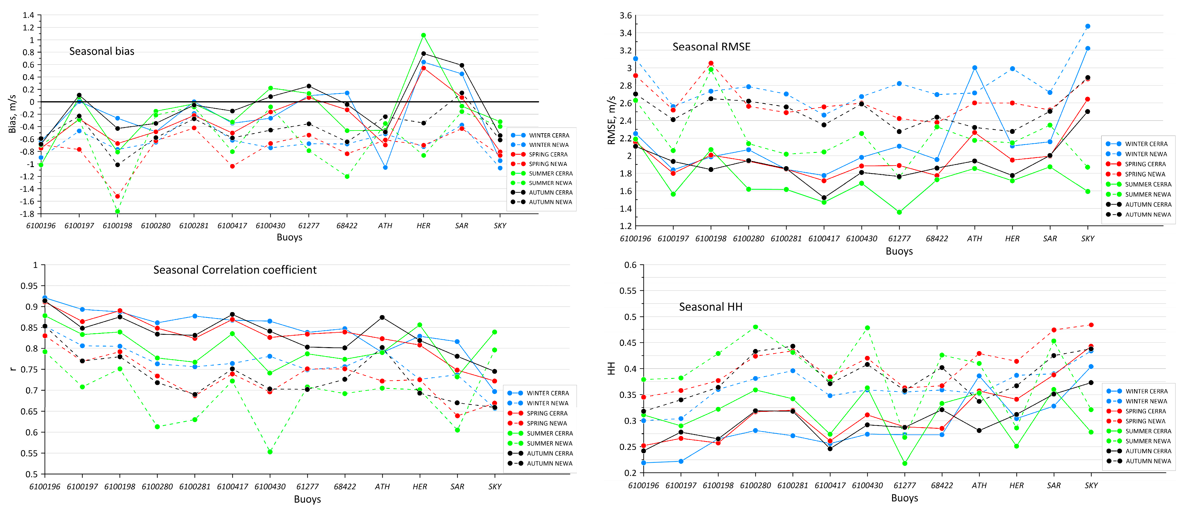
3.2. Seasonal Evaluation

In this section, the seasonal evaluation results of the CERRA and NEWA wind datasets are presented for winter (DJF), spring (MAM), summer (JJA) and autumn (SON) in

Table 10. Seasonal statistical results between collocated CERRA (C) and NEWA (N) models for winter.

Buoy	$\mathit{R}\mathit{M}\mathit{S}\mathit{E}$ (m/s)		$\mathit{b}$ (m/s)		$\mathit{r}$		$\mathit{M}\mathit{A}\mathit{E}$ (m/s)		$\mathit{S}\mathit{I}$		$\mathit{H}\mathit{H}$
	C	N	C	N	C	N	C	N	C	N	C	N
6100196	2.252	3.104	−0.639	−0.898	0.921	0.853	1.630	2.314	0.252	0.346	0.219	0.300
6100197	1.838	2.560	0.005	−0.469	0.893	0.806	1.363	1.881	0.249	0.341	0.222	0.304
6100198	1.987	2.734	−0.265	−0.768	0.887	0.805	1.439	2.060	0.313	0.420	0.265	0.360
6100280	2.068	2.786	−0.482	−0.652	0.861	0.763	1.564	2.141	0.323	0.441	0.281	0.381
6100281	1.844	2.702	0.001	−0.188	0.877	0.756	1.370	2.047	0.315	0.459	0.271	0.396
6100417	1.774	2.463	−0.345	−0.619	0.867	0.764	1.321	1.865	0.290	0.391	0.256	0.348
6100430	1.981	2.673	−0.264	−0.741	0.865	0.781	1.459	1.987	0.317	0.411	0.274	0.359
61277	2.108	2.822	0.099	−0.674	0.838	0.749	1.542	2.069	0.301	0.398	0.273	0.355
68422	1.956	2.696	0.142	−0.680	0.847	0.756	1.475	2.020	0.302	0.404	0.273	0.359
ATH	3.002	2.714	−1.058	−0.517	0.790	0.796	2.004	2.039	0.450	0.409	0.386	0.352
HER	2.111	2.991	0.639	−0.723	0.829	0.726	1.593	2.236	0.308	0.438	0.304	0.387
SAR	2.158	2.720	0.449	−0.375	0.816	0.737	1.644	2.087	0.350	0.447	0.328	0.390
SKY	3.223	3.475	−0.949	−1.066	0.697	0.657	2.105	2.368	0.452	0.486	0.404	0.434

,

Table 11. Seasonal statistical results between collocated CERRA (C) and NEWA (N) models for spring.

Buoy	$\mathit{R}\mathit{M}\mathit{S}\mathit{E}$ (m/s)		$\mathit{b}$ (m/s)		$\mathit{r}$		$\mathit{M}\mathit{A}\mathit{E}$ (m/s)		$\mathit{S}\mathit{I}$		$\mathit{H}\mathit{H}$
	C	N	C	N	C	N	C	N	C	N	C	N
6100196	2.155	2.912	−0.748	−0.694	0.911	0.830	1.583	2.181	0.295	0.412	0.252	0.345
6100197	1.799	2.520	−0.278	−0.768	0.864	0.769	1.330	1.927	0.304	0.404	0.266	0.358
6100198	2.006	3.053	−0.672	−1.521	0.890	0.792	1.471	2.370	0.290	0.406	0.257	0.377
6100280	1.937	2.562	−0.482	−0.628	0.848	0.734	1.438	1.942	0.375	0.498	0.317	0.424
6100281	1.846	2.491	−0.220	−0.421	0.824	0.687	1.364	1.892	0.371	0.499	0.320	0.434
6100417	1.715	2.556	−0.503	−1.038	0.869	0.739	1.278	1.956	0.292	0.420	0.261	0.384
6100430	1.883	2.599	−0.164	−0.671	0.826	0.696	1.400	1.982	0.358	0.478	0.311	0.420
61277	1.888	2.422	0.068	−0.536	0.834	0.751	1.380	1.795	0.321	0.411	0.288	0.363
68422	1.773	2.378	−0.129	−0.837	0.839	0.751	1.304	1.798	0.323	0.407	0.285	0.367
ATH	2.264	2.601	−0.696	−0.615	0.823	0.722	1.657	1.969	0.424	0.502	0.357	0.429
HER	1.950	2.600	0.544	−0.699	0.808	0.725	1.501	1.980	0.352	0.475	0.341	0.414
SAR	1.994	2.520	0.071	−0.432	0.748	0.639	1.512	1.917	0.436	0.543	0.388	0.474
SKY	2.644	2.875	−0.806	−0.864	0.722	0.669	1.793	2.088	0.520	0.566	0.443	0.484

,

Table 12. Seasonal statistical results between collocated CERRA (C) and NEWA (N) models for summer.

Buoy	$\mathit{R}\mathit{M}\mathit{S}\mathit{E}$ (m/s)		$\mathit{b}$ (m/s)		$\mathit{r}$		$\mathit{M}\mathit{A}\mathit{E}$ (m/s)		$\mathit{S}\mathit{I}$		$\mathit{H}\mathit{H}$
	C	N	C	N	C	N	C	N	C	N	C	N
6100196	2.189	2.630	−1.017	−0.697	0.878	0.792	1.633	1.999	0.351	0.448	0.311	0.379
6100197	1.562	2.058	0.078	−0.288	0.833	0.708	1.152	1.558	0.321	0.429	0.290	0.382
6100198	2.069	2.982	−0.809	−1.763	0.839	0.751	1.578	2.347	0.361	0.439	0.322	0.429
6100280	1.618	2.137	−0.152	−0.214	0.777	0.613	1.197	1.614	0.412	0.542	0.359	0.480
6100281	1.616	2.017	−0.033	−0.082	0.767	0.630	1.182	1.519	0.382	0.474	0.342	0.431
6100417	1.470	2.043	−0.326	−0.803	0.835	0.722	1.094	1.585	0.306	0.407	0.274	0.375
6100430	1.686	2.253	0.222	−0.083	0.741	0.553	1.261	1.709	0.387	0.520	0.363	0.478
61277	1.358	1.754	0.135	−0.787	0.787	0.708	1.058	1.327	0.225	0.264	0.218	0.268
68422	1.726	2.328	−0.465	−1.203	0.774	0.692	1.310	1.836	0.371	0.445	0.333	0.426
ATH	1.855	2.174	−0.460	−0.350	0.790	0.705	1.396	1.658	0.408	0.468	0.353	0.410
HER	1.715	2.146	1.075	−0.864	0.856	0.701	1.422	1.505	0.190	0.290	0.251	0.286
SAR	1.873	2.348	−0.071	−0.157	0.732	0.605	1.415	1.803	0.399	0.500	0.360	0.453
SKY	1.593	1.869	−0.321	−0.398	0.839	0.796	1.136	1.373	0.312	0.362	0.278	0.321

, and

Table 13. Seasonal statistical results between collocated CERRA (C) and NEWA (N) models for autumn.

Buoy	$\mathit{R}\mathit{M}\mathit{S}\mathit{E}$ (m/s)		$\mathit{b}$ (m/s)		$\mathit{r}$		$\mathit{M}\mathit{A}\mathit{E}$ (m/s)		$\mathit{S}\mathit{I}$		$\mathit{H}\mathit{H}$
	C	N	C	N	C	N	C	N	C	N	C	N
6100196	2.106	2.703	−0.682	−0.592	0.914	0.853	1.574	2.031	0.283	0.380	0.242	0.318
6100197	1.934	2.411	0.107	−0.229	0.848	0.770	1.349	1.764	0.308	0.383	0.278	0.340
6100198	1.842	2.649	−0.430	−1.014	0.875	0.780	1.382	2.051	0.304	0.405	0.265	0.364
6100280	1.944	2.621	−0.347	−0.577	0.834	0.718	1.454	1.995	0.374	0.508	0.319	0.433
6100281	1.853	2.555	−0.053	−0.274	0.831	0.690	1.343	1.917	0.368	0.511	0.318	0.443
6100417	1.522	2.351	−0.149	−0.582	0.881	0.751	1.117	1.773	0.280	0.422	0.246	0.371
6100430	1.809	2.589	0.083	−0.456	0.841	0.703	1.334	1.930	0.329	0.465	0.292	0.408
61277	1.763	2.274	0.253	−0.354	0.803	0.702	1.265	1.621	0.303	0.395	0.287	0.358
68422	1.859	2.439	−0.043	−0.644	0.801	0.726	1.368	1.825	0.362	0.459	0.321	0.402
ATH	1.940	2.321	−0.487	−0.239	0.874	0.802	1.442	1.688	0.328	0.389	0.281	0.337
HER	1.774	2.276	0.776	−0.342	0.819	0.693	1.377	1.632	0.285	0.405	0.312	0.367
SAR	2.002	2.505	0.588	0.143	0.781	0.670	1.549	1.905	0.353	0.464	0.351	0.425
SKY	2.503	2.890	−0.544	−0.615	0.745	0.659	1.546	1.928	0.425	0.496	0.373	0.438

, respectively, for all examined buoys.

For the winter season, CERRA performs, overall, better than NEWA as regards all the examined statistical measures. Specifically, for $MAE$ and $SI$, CERRA provides the lowest values for all locations, while it provides the lowest values for $RMSE$ and $HH$ and the highest values for $r$ for all locations (except for ATH). For $b$, CERRA provides the lowest values for all locations (except for ATH and SAR).

For the spring season, CERRA performs, overall, and better than NEWA as regards all the examined statistical measures. Specifically, CERRA provides the lowest values for $RMSE$, $SI$, $HH$, and $MAE$, and the highest values for $r$ for all locations, while for $b$ CERRA provides the lowest values for all locations except for ATH.

For the summer season, CERRA provides the lowest values for $RMSE$, $MAE$, $SI$ and $HH$, and the highest values for $r$ for all locations, while for $b$, CERRA provides the lowest values for all locations except for 6100196, 6100430 and ATH.

For the autumn season, CERRA provides the lowest values for $RMSE$, $MAE$, $SI$, and $HH$, and the highest values for $r$ for all locations, while for $b$, it provides the lowest values for all locations except for 6100196, ATH, HER and SAR.

In Figure 2, $b$, $r$, $RMSE$ and $HH$ are depicted for each season and buoy location. Overall, it seems that $RMSE$ and $r$ take lower values during summer and higher values during winter for both CERRA and NEWA. For $HH$, the higher values are overall encountered for summer and the lower values for winter among the buoys of the western Mediterranean. It is also evident that NEWA systematically underestimates wind speed for all seasons and locations (except for SAR for autumn). Also, for the majority of the cases, CERRA underestimates wind speed for all seasons for the buoys of the western Mediterranean, while for the Greek buoys HER and SAR, CERRA overestimates wind speed.

4. Conclusions

In this work, the wind speeds obtained from the CERRA and NEWA datasets have been evaluated for offshore Mediterranean locations at 10 m above sea level, using long-term wind data from 13 oceanographic buoys. Most of the available buoys are located in the western and central eastern Mediterranean and the wind speed data that were obtained from the Copernicus Marine Service have been quality controlled by the providing organizations, and quality flags have been assigned to the values of the wind speed time series.

The evaluation procedure was extensive. First, an evaluation at the hourly scale was performed and then the same process was followed for the seasonal scale. In addition, an evaluation of the collocated data samples with $U_B\ge U_{B,0.90}$ and $U_B\ge U_{B,0.95}$ has also been performed in order to assess the quality of CERRA and NEWA at extreme wind speeds.

The statistical evaluation of the collocated wind speed data from buoys and CERRA has revealed that bias takes relatively low values ranging between –0.780 m/s and 0.796 m/s for CERRA and relatively high (in the absolute sense) values for NEWA ranging between –1.250 m/s and –0.192 m/s. CERRA outperforms NEWA in this respect for 9 out of 13 locations. For CERRA, all $RMSE$ values are below 2.5 m/s, while for NEWA all $RMSE$ values are greater than 2.3 m/s. CERRA outperforms NEWA by providing smaller $RMSE$ values for all locations. $r$ takes systematically medium to high values for CERRA ranging from 0.753 up to 0.912, while for NEWA, $r$ takes medium values with the corresponding range 0.681 to 0.844. CERRA also outperforms NEWA with respect to $MAE$, $SI$ and $HH$ since it provides smaller values for all examined locations. Moreover, at the basin scale, the weighted averages of all the examined statistics clearly suggest the superiority of the CERRA wind dataset, while it seems that there is no systematic behaviour as regards the quality performance of both models (CERRA and NEWA) at the spatial/regional scale.

The same qualitative characteristics have been also observed at the seasonal time scale, where, overall, CERRA clearly outperforms NEWA. NEWA exhibits a better performance only in the following very limited situations: for winter, NEWA outperforms only in ATH (as regards all statistics except for $MAE$); for spring in 6100196 and ATH (as regards the bias); for summer only with respect to bias for 6100196, 6100430, ATH and HER; while for autumn, NEWA outperforms only with respect to bias for 6100196, ATH, HER and SAR.

Regarding the evaluation of the wind speeds greater than the 90th and 95th percentile points, the values of all the evaluation parameters are clearly increased and $r$ is clearly decreased. For $U_B\ge U_{B,0.95}$, CERRA outperforms NEWA with respect to $r$, $MAE$ and $SI$ for all locations, while with respect to $RMSE$ and $HH$, CERRA outperforms NEWA for 12 out of 13 locations. For $b$, CERRA outperforms NEWA for seven locations. For $U_B\ge U_{B,0.95}$, CERRA outperforms NEWA with respect to $r$ and $SI$ for all locations; with respect to $HH$, CERRA outperforms NEWA for 12 locations; with respect to $MAE$ and $RMSE$, it outperforms NEWA for 11 out of 13 locations; and with respect to $b$, CERRA outperforms NEWA for 8 locations. However, both datasets show increased errors and reduced correlation in the upper tail of the wind speed distribution, which is expected since extreme events are harder to simulate; this suggests caution in using these datasets for extreme wind prediction, a critical consideration for turbine structural design. In this connection, it is suggested to use CERRA for general resource assessment, but neither of the examined datasets may be highly accurate at predicting the absolute highest wind events without further bias correction or modelling.

The results of this analysis establish CERRA as the more reliable model for replicating buoy measured winds in the Mediterranean Sea, at least for the regions of the Mediterranean where validation data were available, and guide practitioners toward CERRA for baseline wind resource assessment. Our results align with recent findings that newer regional reanalyses (like CERRA) provide substantial error reductions over older or coarser reanalyses (e.g., ERA5). This highlights the progress in wind resource modelling and the benefit of high-resolution data for offshore wind applications.

The superior performance of CERRA is likely attributable to its data assimilation of in situ and satellite wind observations, which continuously correct the model trajectory, whereas NEWA’s free WRF simulations (despite higher nominal resolution) may accumulate biases. The systematic underestimation by NEWA suggests a possible bias in the WRF configuration or the climatology of its forcing; this aligns with findings from other studies (e.g., [31]) that noted WRF-based wind atlases can underestimate wind speed in certain regions. Further investigation into the NEWA model setup (surface layer schemes, etc.) could explain this bias. Let us also remember that the lateral boundary conditions for NEWA are from ERA-Interim [38], i.e., a reanalysis product of lower quality compared to ERA5. In these respects, adjusting the model’s roughness or applying a bias correction could improve its utility for wind resource assessments.

Some important future steps of this work are (i) to obtain validation data in the central Mediterranean in order to confirm that the current conclusions hold everywhere across the basin, combined with an analysis including ERA5 wind data; (ii) to assess in depth the regional behaviour of both models at the Mediterranean basin level.

References

1. Soukissian, T.; Papadopoulos, A.; Skrimizeas, P.; Karathanasi, F.; Axaopoulos, P.; Avgoustoglou, E.; Kyriakidou, H.; Tsalis, C.; Voudouri, A.; Gofa, F.; et al. Assessment of offshore wind power potential in the Aegean and Ionian Seas based on high-resolution hindcast model results. AIMS Energy 2017, 5, 268–289. [Google Scholar] [CrossRef]
2. Soukissian, T.H.; Karathanasi, F.E.; Zaragkas, D.K. Exploiting offshore wind and solar resources in the Mediterranean using ERA5 reanalysis data. Energy Convers. Manag. 2021, 237, 114092. [Google Scholar] [CrossRef]
3. Kardakaris, K.; Boufidi, I.; Soukissian, T. Offshore Wind and Wave Energy Complementarity in the Greek Seas Based on ERA5 Data. Atmosphere 2021, 12, 1360. [Google Scholar] [CrossRef]
4. Zheng, C.-W.; Xiao, Z.-N.; Peng, Y.-H.; Li, C.-Y.; Du, Z.-B. Rezoning global offshore wind energy resources. Renew. Energy 2018, 129, 1–11. [Google Scholar] [CrossRef]
5. Zheng, C.W.; Pan, J. Assessment of the global ocean wind energy resource. Renew. Sustain. Energy Rev. 2014, 33, 382–391. [Google Scholar] [CrossRef]
6. Medina-Lopez, E.; McMillan, D.; Lazic, J.; Hart, E.; Zen, S.; Angeloudis, A.; Bannon, E.; Browell, J.; Dorling, S.; Dorrell, R.M.; et al. Satellite data for the offshore renewable energy sector: Synergies and innovation opportunities. Remote Sens. Environ. 2021, 264, 112588. [Google Scholar] [CrossRef]
7. Soukissian, T.; Karathanasi, F.; Axaopoulos, P. Satellite-Based Offshore Wind Resource Assessment in the Mediterranean Sea. IEEE J. Ocean. Eng. 2017, 42, 73–86. [Google Scholar] [CrossRef]
8. Li, X.; Mitsopoulos, P.; Yin, Y.; Peña, M. SARAL-AltiKa Wind and Significant Wave Height for Offshore Wind Energy Applications in the New England Region. Remote Sens. 2021, 13, 57. [Google Scholar] [CrossRef]
9. Ahsbahs, T.; Badger, M.; Volker, P.; Hansen, K.S.; Hasager, C.B. Applications of satellite winds for the offshore wind farm site Anholt. Wind Energy Sci. 2018, 3, 573–588. [Google Scholar] [CrossRef]
10. de Baar, J.; Nhat Luu, L.; van der Schrier, G.; van den Besselaar, E.; Garcia-Marti, I. Recent improvements in the E-OBS gridded data set for daily mean wind speed over Europe in the period 1980–2021. In Proceedings of the EMS Annual Meeting 2022, Bonn, Germany, 4–9 September 2022. [Google Scholar]
11. Zhang, H.; Jeffrey, S.; Carter, J. Improved quality gridded surface wind speed datasets for Australia. Meteorol. Atmos. Phys. 2022, 134, 85. [Google Scholar] [CrossRef]
12. Gualtieri, G. Analysing the uncertainties of reanalysis data used for wind resource assessment: A critical review. Renew. Sustain. Energy Rev. 2022, 167, 112741. [Google Scholar] [CrossRef]
13. Muñoz-Sabater, J.; Dutra, E.; Agustí-Panareda, A.; Albergel, C.; Arduini, G.; Balsamo, G.; Boussetta, S.; Choulga, M.; Harrigan, S.; Hersbach, H.; et al. ERA5-Land: A state-of-the-art global reanalysis dataset for land applications. Earth Syst. Sci. Data 2021, 13, 4349–4383. [Google Scholar] [CrossRef]
14. Vousdoukas, M.I.; Voukouvalas, E.; Annunziato, A.; Giardino, A.; Feyen, L. Projections of extreme storm surge levels along Europe. Clim. Dyn. 2016, 47, 3171–3190. [Google Scholar] [CrossRef]
15. Ren, G.; Wan, J.; Liu, J.; Yu, D. Characterization of wind resource in China from a new perspective. Energy 2019, 167, 994–1010. [Google Scholar] [CrossRef]
16. He, J.; Chan, P.W.; Li, Q.; Lee, C.W. Spatiotemporal analysis of offshore wind field characteristics and energy potential in Hong Kong. Energy 2020, 201, 117622. [Google Scholar] [CrossRef]
17. Salvação, N.; Guedes Soares, C. Wind resource assessment offshore the Atlantic Iberian coast with the WRF model. Energy 2018, 145, 276–287. [Google Scholar] [CrossRef]
18. Schimanke, S.; Ridal, M.; Le Moigne, P.; Berggren, L.; Undén, P.; Randriamampianina, R.; Andrea, U.; Bazile, E.; Bertelsen, A.; Brousseau, P.; et al. CERRA Sub-Daily Regional Reanalysis Data for Europe on Single Levels from 1984 to Present; Copernicus Climate Change Service (C3S) Climate Data Store (CDS): Bonn, Germany, 2021; Available online: https://cds.climate.copernicus.eu/cdsapp#!/dataset/reanalysis-cerra-single-levels?tab=overview (accessed on 10 January 2025).
19. Dee, D.P.; Uppala, S.M.; Simmons, A.J.; Berrisford, P.; Poli, P.; Kobayashi, S.; Andrae, U.; Balmaseda, M.A.; Balsamo, G.; Bauer, P.; et al. The ERA-Interim reanalysis: Configuration and performance of the data assimilation system. Q. J. R. Meteorol. Soc. 2011, 137, 553–597. [Google Scholar] [CrossRef]
20. Hersbach, H.; Bell, B.; Berrisford, P.; Hirahara, S.; Horányi, A.; Muñoz-Sabater, J.; Nicolas, J.; Peubey, C.; Radu, R.; Schepers, D.; et al. The ERA5 global reanalysis. Q. J. R. Meteorol. Soc. 2020, 146, 1999–2049. [Google Scholar] [CrossRef]
21. Galanaki, E.; Giannaros, C.; Agathangelidis, I.; Cartalis, C.; Kotroni, V.; Lagouvardos, K.; Matzarakis, A. Validating the Copernicus European Regional Reanalysis (CERRA) Dataset for Human-Biometeorological Applications. Environ. Sci. Proc. 2023, 26, 111. [Google Scholar] [CrossRef]
22. Hadjipetrou, S.; Kyriakidis, P. High-Resolution Wind Speed Estimates for the Eastern Mediterranean Basin: A Statistical Comparison Against Coastal Meteorological Observations. Wind 2024, 4, 311–341. [Google Scholar] [CrossRef]
23. Rouholahnejad, F.; Meyer, P.; Gottschall, J. Collocating wind data: A case study on the verification of the CERRA dataset. J. Phys. Conf. Ser. 2024, 2875, 012016. [Google Scholar] [CrossRef]
24. Pelosi, A. Performance of the Copernicus European Regional Reanalysis (CERRA) dataset as proxy of ground-based agrometeorological data. Agric. Water Manag. 2023, 289, 108556. [Google Scholar] [CrossRef]
25. Jourdier, B.; Diaz, C.; Dubus, L. Evaluation of CERRA for wind energy applications. In Proceedings of the EMS Annual Meeting 2023, Bratislava, Slovakia, 4–9 September 2023. [Google Scholar]
26. Spangehl, T.; Borsche, M.; Niermann, D.; Kaspar, F.; Schimanke, S.; Brienen, S.; Möller, T.; Brast, M. Intercomparing the quality of recent reanalyses for offshore wind farm planning in Germany’s exclusive economic zone of the North Sea. Adv. Sci. Res. 2023, 20, 109–128. [Google Scholar] [CrossRef]
27. Hahmann, A.N.; Sīle, T.; Witha, B.; Davis, N.N.; Dörenkämper, M.; Ezber, Y.; García-Bustamante, E.; González-Rouco, J.F.; Navarro, J.; Olsen, B.T.; et al. The making of the New European Wind Atlas—Part 1: Model sensitivity. Geosci. Model Dev. 2020, 13, 5053–5078. [Google Scholar] [CrossRef]
28. Skamarock, W.; Klemp, J.; Dudhia, J.; Gill, D.O.; Barker, D.; Duda, M.G.; Huang, X.-Y.; Wang, W.; Powers, J.G. A Description of the Advanced Research WRF Version 3; University Corporation for Atmospheric Research: Boulder, CO, USA, 2008. [Google Scholar]
29. Murcia, J.P.; Koivisto, M.J.; Luzia, G.; Olsen, B.T.; Hahmann, A.N.; Sørensen, P.E.; Als, M. Validation of European-scale simulated wind speed and wind generation time series. Appl. Energy 2022, 305, 117794. [Google Scholar] [CrossRef]
30. Kalverla, P.C.; Holtslag, A.A.M.; Ronda, R.J.; Steeneveld, G.-J. Quality of wind characteristics in recent wind atlases over the North Sea. Q. J. R. Meteorol. Soc. 2020, 146, 1498–1515. [Google Scholar] [CrossRef]
31. Meyer, P.J.; Gottschall, J. How do NEWA and ERA5 compare for assessing offshore wind resources and wind farm siting conditions? J. Phys. Conf. Ser. 2022, 2151, 012009. [Google Scholar] [CrossRef]
32. Araveti, S.; Quintana, C.A.; Kairisa, E.; Mutule, A.; Adriazola, J.P.S.; Sweeney, C.; Carroll, P. Wind Energy Assessment for Renewable Energy Communities. Wind 2022, 2, 325–347. [Google Scholar] [CrossRef]
33. Jourdier, B. Evaluation of ERA5, MERRA-2, COSMO-REA6, NEWA and AROME to simulate wind power production over France. Adv. Sci. Res. 2020, 17, 63–77. [Google Scholar] [CrossRef]
34. Ridal, M.; Bazile, E.; Le Moigne, P.; Randriamampianina, R.; Schimanke, S.; Andrae, U.; Berggren, L.; Brousseau, P.; Dahlgren, P.; Edvinsson, L.; et al. CERRA, the Copernicus European Regional Reanalysis system. Q. J. R. Meteorol. Soc. 2024, 150, 3385–3411. [Google Scholar] [CrossRef]
35. Wang, Z.Q.; Randriamampianina, R. The Impact of Assimilating Satellite Radiance Observations in the Copernicus European Regional Reanalysis (CERRA). Remote Sens. 2021, 13, 426. [Google Scholar] [CrossRef]
36. El-Said, A.; Brousseau, P.; Ridal, M.; Randriamampianina, R. Towards Full Flow-Dependence: New Temporally Varying EDA Quotient Functionality to Estimate Background Errors in CERRA. J. Adv. Model. Earth Syst. 2022, 14, e2021MS002637. [Google Scholar] [CrossRef]
37. Calamia, J. Where the wind blows. New Sci. 2017, 234, 31–33. [Google Scholar] [CrossRef]
38. Karagali, I.; Hahmann, A.N.; Badger, M.; Hasager, C.; Mann, J. New European wind atlas offshore. J. Phys. Conf. Ser. 2018, 1037, 052007. [Google Scholar] [CrossRef]
39. Mann, J.; Angelou, N.; Arnqvist, J.; Callies, D.; Cantero, E.; Chávez Arroyo, R.; Courtney, M.; Cuxart, J.; Dellwik, E.; Gottschall, J.; et al. Complex terrain experiments in the New European Wind Atlas. Philos. Trans. R. Soc. A Math. Phys. Eng. Sci. 2017, 375. [Google Scholar] [CrossRef] [PubMed]
40. Olsen, B.T.; Hahmann, A.N.; Sempreviva, A.M.; Badger, J.; Jørgensen, H.E. An intercomparison of mesoscale models at simple sites for wind energy applications. Wind Energy Sci. 2017, 2, 211–228. [Google Scholar] [CrossRef]
41. Dörenkämper, M.; Olsen, B.T.; Witha, B.; Hahmann, A.N.; Davis, N.N.; Barcons, J.; Ezber, Y.; García-Bustamante, E.; González-Rouco, J.F.; Navarro, J.; et al. The Making of the New European Wind Atlas—Part 2: Production and evaluation. Geosci. Model Dev. 2020, 13, 5079–5102. [Google Scholar] [CrossRef]
42. Soukissian, T.H.; Chronis, G.T.; Nittis, K.; Diamanti, C. Advancement of Operational Oceanography in Greece: The Case of the Poseidon System. J. Atmos. Ocean Sci. 2002, 8, 93–107. [Google Scholar] [CrossRef]
43. Copernicus Marine in Situ tac Data Management Team, NetCDF Format Manual Version 2.0.0. 2023, p. 28. Available online: https://archimer.ifremer.fr/doc/00488/59938/ (accessed on 10 January 2025).
44. Mears, C.A.; Smith, D.K.; Wentz, F. Comparison of Special Sensor Microwave Imager and buoy-measured wind speeds from 1987 to 1997. J. Geophys. Res. 2001, 106, 719–729. [Google Scholar] [CrossRef]
45. Peng, G.; Zhang, H.-M.; Frank, H.P.; Bidlot, J.-R.; Higaki, M.; Stevens, S.; Hankins, W.R. Evaluation of Various Surface Wind Products with OceanSITES Buoy Measurements. Weather Forecast. 2013, 28, 1281–1303. [Google Scholar] [CrossRef]
46. Shu, Z.R.; Li, Q.S.; He, Y.C.; Chan, P.W. Observations of offshore wind characteristics by Doppler-LiDAR for wind energy applications. Appl. Energy 2016, 169, 150–163. [Google Scholar] [CrossRef]
47. Hansen, F.V. Surface Roughness Lengths; U.S. Army Research Laboratory, White Sands Missile Range: Las Cruces, NM, USA, 1993; pp. 1–40. [Google Scholar]
48. Mortensen, N.G.; Landberg, L.; Troen, I.; Petersen, E.L. Wind Analysis and Application Program (WAsP)–User’s Guide (Tech. Rep. I-666(EN)); Risø National Laboratory: Roskilde, Denmark, 1993. [Google Scholar]
49. Kim, Y.-H.; Lim, H.-C. Effect of island topography and surface roughness on the estimation of annual energy production of offshore wind farms. Renew. Energy 2017, 103, 106–114. [Google Scholar] [CrossRef]
50. Golbazi, M.; Archer, C.L. Methods to Estimate Surface Roughness Length for Offshore Wind Energy. Adv. Meteorol. 2019, 2019, 5695481. [Google Scholar] [CrossRef]
51. Mentaschi, L.; Besio, G.; Cassola, F.; Mazzino, A. Problems in RMSE-based wave model validations. Ocean Model. 2013, 72, 53–58. [Google Scholar] [CrossRef]
52. Hanna, S.R.; Heinold, D.W. Development and Application of a Simple Method for Evaluating Air Quality Models; American Petroleum Institute: Washington, DC, USA, 1985. [Google Scholar]
Figure 1. Locations of the examined oceanographic buoys. Green colour: Spanish buoys, blue colour: Greek buoys.
Jmse 13 01445 g001
Figure 2. Seasonal statistical metrics for all examined locations.
Jmse 13 01445 g002