A Heave Motion Prediction Approach Based on Sparse Bayesian Learning Incorporated with Empirical Mode Decomposition for an Underwater Towed System

Abstract

Underwater towed systems (UTSs) are widely used in underwater exploration and oceanographic data acquisition. However, the heave motion information of the towing ship is usually affected by the measurement transmitting delay, sensor noise and surface waves, which will result in uncontrolled depth variation of the towed vehicle, so as to adversely affect the monitoring performance and mechanical robustness of the UTS. To resolve this problem, a heave motion prediction approach based on sparse Bayesian learning (SBL) incorporated with empirical mode decomposition (EMD) for the UTS is proposed in this paper. With the proposed approach, a heave motion model of the towing ship with random waves is firstly developed based on strip theory. Meanwhile, the EMD is employed to eliminate the high-frequency noise of the measurement data to restore low-frequency towing ship motion. And then, the SBL is utilized to train the weight parameters in the built model to predict the heave motion, which not only reconstruct the heave motion from non-stationary sensor signals with noise but also prevent overfitting. Furthermore, the depth compensation of the towed vehicle is then performed using the predicted heave motion. Finally, experimental results demonstrate that the proposed EMD-SBL method significantly improves both the prediction accuracy and model adaptability under various sea conditions, and it also guarantees that the maximum prediction depth error of the heave motion does not exceed 1 cm.

1. Introduction

Underwater towed systems (UTSs) (shown in Figure 1) are widely used in the field of underwater environment exploration and oceanographic data acquisition [1,2]. However, the sensor delay prevents real-time feedback on the motion of the towing ship induced by surface waves. Consequently, the system is unable to dynamically adjust the depth of the towed vehicle by retracting or releasing the towing cable based on sensor inputs. This limitation leads to variations in the depth of the towed vehicle, which in turn affects its exploring performance [3]. Given that the roll and pitch motions of the towing ship can be effectively managed by its power positioning system [4], accurately predicting the heave motion of the towing ship is of great significance for the further application of a UTS.

To this end, four ship motion prediction methods have been well-understood and developed to date: hydrodynamic-based models, classic time-series prediction models, intelligent nonlinear learning models, and hybrid models [5]. System identification-wise, all models can be classified into statistical models (black box approach) and a physical process (white/gray box approach). The statistical model-based methods mainly include time-series analysis, such as the autoregressive model, AR [6], autoregressive moving average model, ARMA [4], autoregressive integrated moving average model, ARIMA [7], and machine learning-based methods such as neural network models [8,9,10,11,12], support vector regression, SVR [13], and Gaussian process regression, GPR [14]. However, the omission of physical modeling will result in the loss of the model’s foundational prior information, which will consequently raise significant concerns about the model’s explainability and reliability. Moreover, the limited adaptability of these models undermines their effectiveness in predicting ship motions under different sea conditions.

Physical model-based schemes include potential flow theory-based methods, such as two-dimensional strip methods [15] and three-dimensional panel methods [16,17,18], and viscous flow theory-based methods, such as Reynolds-averaged Navier–Stokes methods, RANS [19]. However, the nonlinearity of ship motion models in marine environments can impede the direct acquisition of model parameters. Furthermore, traditional parameter estimation methods, such as least squares [20], are unable to determine the fewest terms required from samples. This limitation can result in overfitting and potentially compromise the accuracy of the model. Furthermore, high-frequency sensor noise can negatively impact the prediction of relatively low-frequency ship motion. Some studies have employed frequency-domain methods, such as Fourier transform [21], for data processing. However, the deficiency of the Fourier-based model is due to the linear decomposition of the signals. In turn, a number of researchers have utilized EMD in conjunction with conventional models for ship motion prediction, due to its ability to obtain non-stationary signals processing [22].

Given that SBL can determine the fewest terms in the past samples required for prediction to avoid overfitting [23], it holds promise in the accurate prediction of heave motion. Further, an EMD-SBL algorithm is proposed to deal with non-stationary signals containing sensor noise. This algorithm enhances the prediction accuracy of heave motion with noise. The main contributions of this article are as follows:

• A simplified heave motion model of a towing ship is developed based on strip theory, and an approach for parameter estimation is proposed, thereby enhancing the prediction reliability and model adaptability.
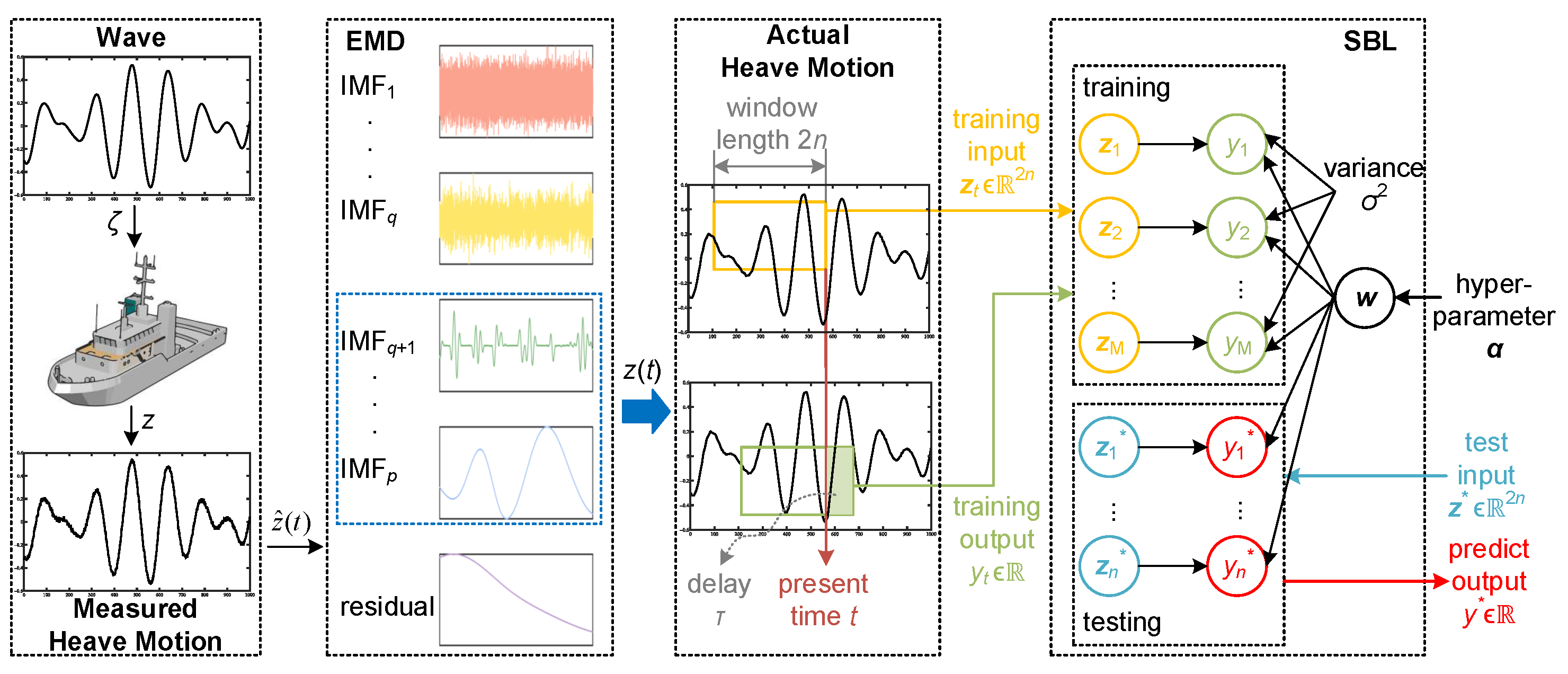
• The EMD is employed to eliminate the high-frequency noise of the measurement data to restore low-frequency towing ship motion. Meanwhile, the SBL is utilized to train the weight parameters in the built model to predict heave motion, which not only reconstruct heave motion from non-stationary sensor signals with noise but also prevent overfitting.
• The depth compensation of the towed vehicle is then performed using the predicted heave motion. Moreover, the compensation results show that the predicted depth compensation effect of the towed vehicle is significantly superior to that without prediction.

2. System Modeling and Problem Formulation

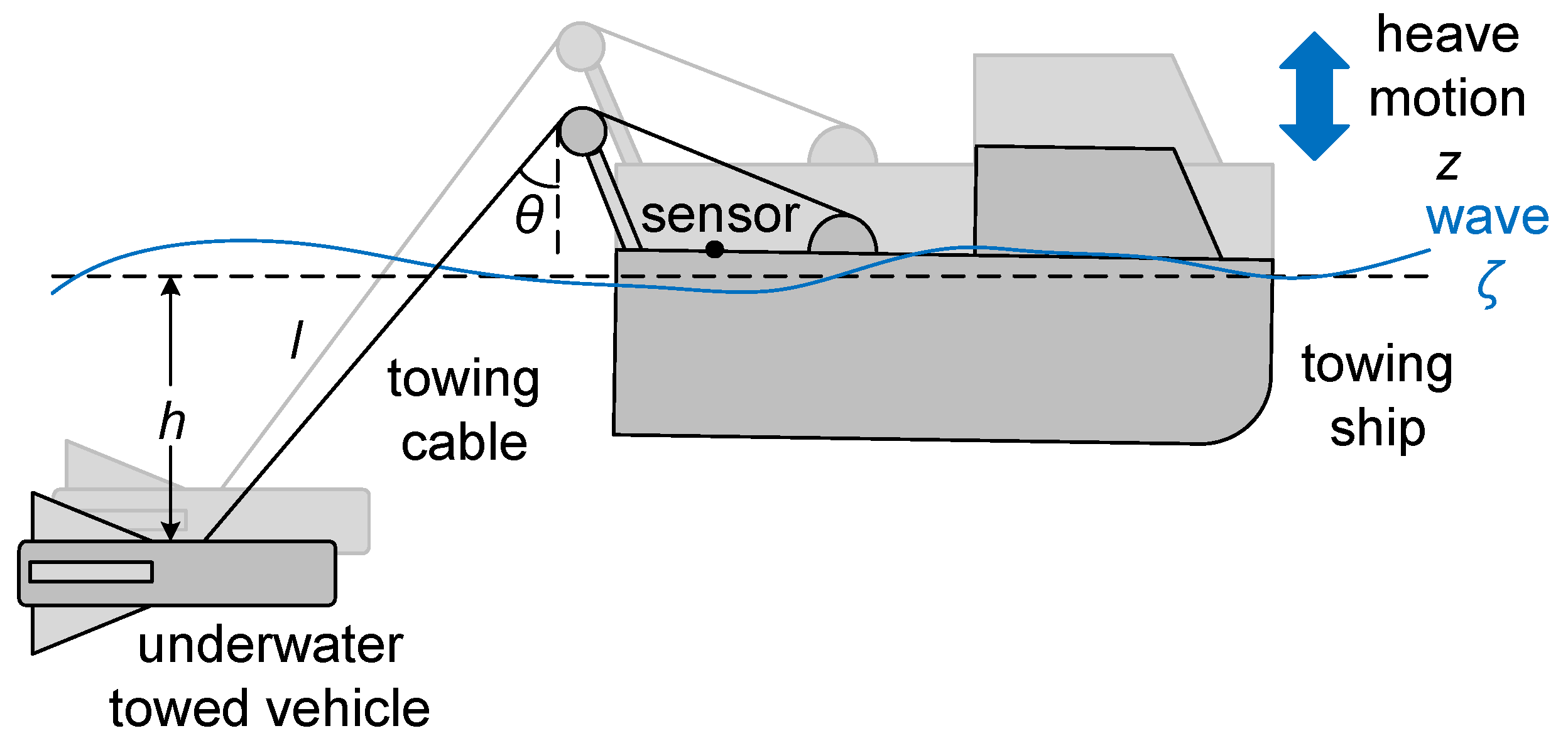
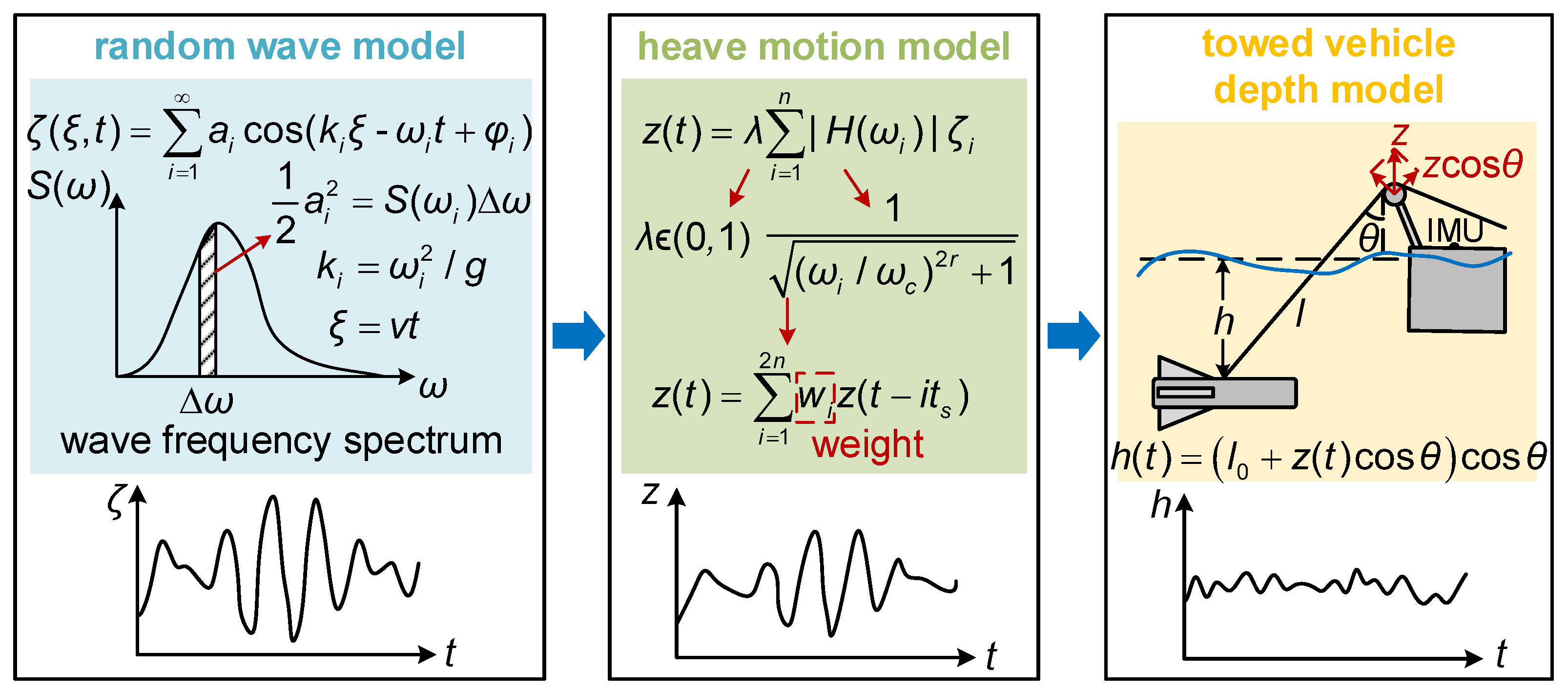
2.1. System Modeling

As shown in Figure 1, the UTS is composed of a towing ship and an underwater towed vehicle connected by a towing cable. The towing ship serves as the power unit of the UTS to provide the necessary towing force to propel the system forward. It is equipped with sensors to capture its motion. The underwater towed vehicle is used for exploration missions. Based on this construction, the system model consists of three main parts, the random wave model, the heave motion model of the towing ship, and the depth model of the towed vehicle, as shown in Figure 2. The random wave model characterizes the wave heights at specific times and positions. The heave motion model describes the heave displacement of the towing ship induced by random waves. The towed vehicle depth model illustrates the depth variation of the towed vehicle caused by the heave motion of the towing ship.

2.1.1. Random Wave Model

As random surface waves will cause uncertain heave motion of the towing ship, to describe the heave motion of the towing ship under random waves, we analyze the wave as it travels along a fixed direction $\xi$. The wave’s height $\zeta$ at a certain position on the sea surface can be approximately described as the sum of cosine waves with amplitude $a_i$, frequency ${\omega }_i$ and initial phase ${\phi }_i$ [11]:

$$\zeta (\xi ,t)=\sum _{i=1}^{\infty }{a}_{i}cos(k_i\xi -{\omega }_{i}t+{\phi }_i)$$

(1)

where $\zeta (\xi ,t)$ is the height of the wave relative to the stationary water surface at a fixed position $\xi$ at time t. $a_i$, $k_i$, ${\omega }_i$, and ${\phi }_i$ are the amplitude, wave number, angular frequency and initial phase of the i-th cosine wave, respectively. ${\phi }_i$ is a random variable in $(0,2\pi )$. $k_i$ and ${\omega }_i$ comply with $k_i={\omega }_i^2/g$.

For a ship moving in a straight line at a uniform speed, its position is proportional to time, as follows:

$$\xi =vt$$

(2)

where v is the speed of the towing ship.

If we only consider the distribution of wave energy relative to frequency, the relationship between the amplitude and energy of a single-frequency component according to the energy equality relationship is

$${\displaystyle \frac{1}{2}}{a}_i^2=S\left({\omega }_i\right)({\omega }_{i+1}-{\omega }_i)$$

(3)

where $S\left(\omega \right)$ is the spectral function of waves.

Substitute $k_i$ and Equations (2) and (3) into Equation (1) with a limited number of harmonics. The wave height at position $\zeta$ is as follows:

$$\begin{array}{cc}\hfill & \zeta \left(t\right)=\sum _{i=1}^n{\zeta }_i\left(t\right)\hfill \\ =\hfill & \sum _{i=1}^n\sqrt{2S\left({\omega }_i\right)({\omega }_{i+1}-{\omega }_i)}cos[({\displaystyle \frac{{\omega }_i^2}{g}}v-{\omega }_i)t+{\phi }_i]\hfill \end{array}$$

(4)

where $\zeta \left(t\right)$ is the height of the wave at time t, ${\zeta }_i\left(t\right)$ is the i-th harmonic component of wave, and n is the number of harmonics.

2.1.2. Heave Motion Model with Random Surface Wave

In order to eliminate the negative influence of heave motion, this section introduces strip theory [15] to model heave motion with a random surface wave. Heave motion of the towing ship established by strip theory in waves [11] is

$$z\left(t\right)=\sum _{i=1}^n\left|W_z\left(j{\omega }_i\right)\right|{\zeta }_i\left(t\right)$$

(5)

where $z\left(t\right)$ is the heave motion of the towing ship, and $|W_z\left(j{\omega }_i\right)|$ is the amplitude–frequency response function of heave motion.

The inertia of the towing ship will result in a reduction in its heave displacement compared to the wave height. Additionally, the high-frequency components of waves will not be reflected in the motion of the towing ship, with only low-frequency components being retained. Hence, the amplitude–frequency response function of the towing ship can be simplified by a low-pass filter [23] with an amplitude attenuation coefficient, as follows:

$$\left|W_z\left(j{\omega }_i\right)\right|=\lambda \left|H\left({\omega }_i\right)\right|$$

(6)

where $\lambda$ is the amplitude attenuation coefficient satisfying $\lambda \in (0,1)$. $H\left(\omega \right)$ is the amplitude–frequency response function of the low-pass filter, which is equal to ${\displaystyle \frac{1}{\sqrt{{\left(\omega /{\omega }_c\right)}^{2r}+1}}}$, in which ${\omega }_c$ and r are the cut-off angular frequency and the order of the filter, respectively. Subsequently, substituting Equations (4) and (6) into Equation (5) yields

$$\begin{array}{cc}\hfill & z\left(t\right)=\sum _{i=1}^n{z}_i\left(t\right)=\lambda \sum _{i=1}^n\left|H\left({\omega }_i\right)\right|{\zeta }_i\hfill \\ \hfill & =\lambda \sum _{i=1}^n\sqrt{{\displaystyle \frac{2S\left({\omega }_i\right)({\omega }_{i+1}-{\omega }_i)}{{\left({\omega }_i/{\omega }_c\right)}^{2r}+1}}}cos[({\displaystyle \frac{{\omega }_i^2}{g}}v-{\omega }_i)t+{\phi }_i]\hfill \end{array}$$

(7)

where $z\left(t\right)$ is the heave motion of the towing ship.

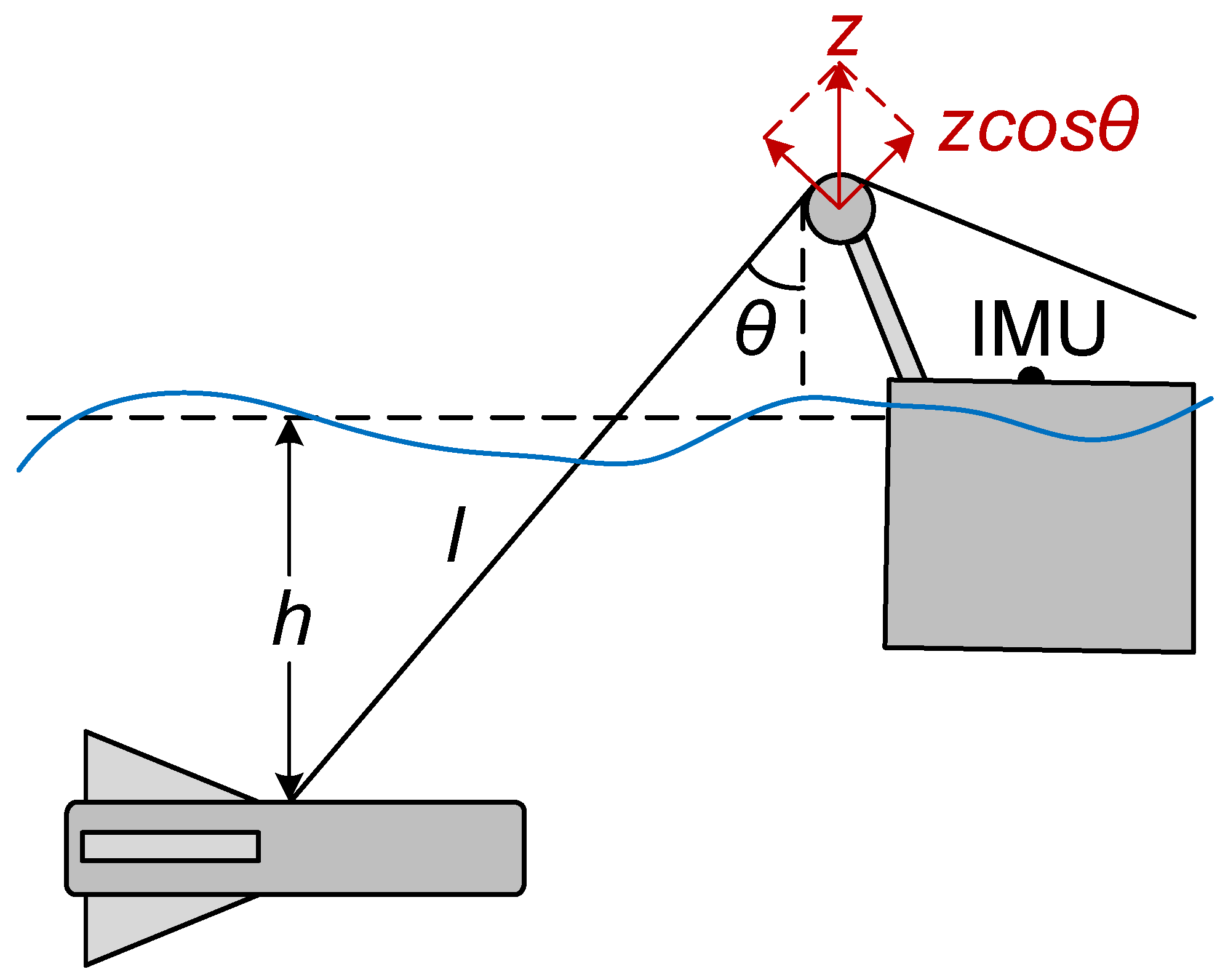
2.1.3. The Depth Model of the Towed Vehicle

In order to demonstrate the effect of heave motion prediction on the towed vehicle’s depth compensation, a depth model of the towed vehicle based on geometric relationships should be developed.

Given the minimal improvement in the towed vehicle’s depth compensation for real-time measurements of the towing cable angle $\theta$ [24], it can be assumed that $\theta$ remains constant. Based on the geometric relationship, the depth model of the towed vehicle is constructed and illustrated in Figure 3.

Since the above-water cable length is much smaller than the underwater length, the depth of the towed vehicle can be expressed as follows:

$$h\left(t\right)=(l_0+z\left(t\right)cos\theta )cos\theta$$

(8)

where $l_0$ is the initial length of cable, $z\left(t\right)$ is the heave motion of the towing ship, $\theta$ is the angle between the cable and the vertical direction, and $h\left(t\right)$ is the depth of the towed vehicle.

Based on the optimal algorithm for determining the retracted or released length of the towing cable, as described in reference [24], the length can be calculated as follows:

$$\Delta l\left(t\right)=-z\left(t\right)cos\theta$$

(9)

where $\Delta l\left(t\right)$ is the adjusting length of cable.

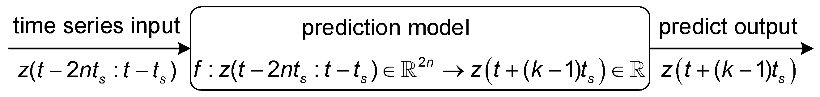
2.2. Problem Formulation

According to Equation (7), the prediction of heave motion requires the estimation of the amplitude, frequency, and phase of each cosine component. The model involves numerous parameters and exhibits significant nonlinear characteristics, making parameter estimation challenging. Thus, in order to facilitate parameter estimation, Equation (7) would be better modified and simplified.

Firstly, $z\left(t\right)$ can be re-expressed as Equation (10), namely the solution of the differential equation. The initial condition ${\mathit{x}}_0$ is determined by the amplitude, frequency and phase of each component.

$$\begin{array}{c}\dot{\mathit{x}}=\mathbf{A}\mathit{x}\hfill \\ z=\mathbf{C}\mathit{x},\mathit{x}\left(0\right)={\mathit{x}}_0\hfill \end{array}$$

(10)

where $\mathit{x}$ is the solution vector composed of heave displacement and its first derivative, $\mathbf{A}$ is the coefficient matrix, $\mathbf{C}$ is the output matrix, and ${\mathit{x}}_0$ is the initial condition. Their expressions are as follows: $\mathit{x}={[z_1{\dot{z}}_1\cdots z_n{\dot{z}}_n]}^{\mathrm{T}}$, $\mathbf{C}=[10\cdots 10]$, ${\mathit{x}}_0={[x_{0,1}{x}_{0,2}\cdots x_{0,2n-1}{x}_{0,2n}]}^{\mathrm{T}}$, $x_{0,2i-1}=\lambda \sqrt{{\displaystyle \frac{2S\left({\omega }_i\right)({\omega }_{i+1}-{\omega }_i)}{{\left({\omega }_i/{\omega }_c\right)}^{2r}+1}}}cos{\phi }_i$, $x_{0,2i}=\lambda \sqrt{{\displaystyle \frac{2S\left({\omega }_i\right)({\omega }_{i+1}-{\omega }_i)}{{\left({\omega }_i/{\omega }_c\right)}^{2r}+1}}}({\omega }_i-{\omega }_i^{2}v/g)sin{\phi }_i$, $i=1,\dots ,n$,

$$\mathbf{A}=\left(\begin{array}{ccccc}0& 1& \cdots & 0& 0\\ {\omega }_1-{\omega }_1^{2}v/g& 0& \cdots & 0& 0\\ ⋮& ⋮& \ddots & ⋮& ⋮\\ 0& 0& \cdots & 0& 1\\ 0& 0& \cdots & {\omega }_n-{\omega }_n^{2}v/g& 0\end{array}\right).$$

Then, transforming Equation (10) into the s-domain yields

$$Z\left(s\right)=\mathbf{C}{(s\mathbf{I}-\mathbf{A})}^{-1}{\mathit{x}}_0=\sum _{i=1}^n{\displaystyle \frac{s{x}_{0,2i-1}+x_{0,2i}}{s^2+{({\omega }_i^{2}v/g-{\omega }_i)}^2}}$$

(11)

After applying the bilinear transformation [25] and substituting $s={\displaystyle \frac{2(z-1)}{t_s(z+1)}}$ into Equation (11), this yields

$$\begin{array}{cc}Z\left(z\right)\hfill & =\sum _{i=1}^n{\displaystyle \frac{(2t_s{x}_{0,2i-1}+x_{0,2i}{t}_s^2)+2x_{0,2i}{t}_s^2{z}^{-1}+(x_{0,2i}{t}_s^2-2t_s{x}_{0,2i-1})z^{-2}}{[4+{({\omega }_i-{\omega }_i^2/g)}^2{t}_s^2]+[2{({\omega }_i-{\omega }_i^2/g)}^2{t}_s^2-8]z^{-1}+[4+{({\omega }_i-{\omega }_i^2/g)}^2{t}_s^2]z^{-2}}}\hfill \\ \hfill & =\sum _{i=0}^{2n}{\displaystyle \frac{b_i{z}^{-i}}{a_i{z}^{-i}}}\hfill \end{array}$$

(12)

where $a_i,b_i,i=0,\dots ,2n$ are coefficients related to the initial condition ${\mathit{x}}_0$ and the sampling period $t_s$.

Write Equation (12) as a difference equation:

$$\sum _{i=0}^{2n}{a}_i{z}^{-i}Z\left(z\right)=\sum _{i=0}^{2n}{b}_i{z}^{-i}$$

(13)

Perform the inverse z-transform on Equation (13):

$$\sum _{i=0}^{2n}{a}_{i}z(t-i{t}_s)=\sum _{i=0}^{2n}{b}_i\delta (t-i{t}_s)$$

(14)

The prediction starts after obtaining $2n$ sampling data, i.e., $t>2n{t}_s$, so $\delta \left(t\right)=\delta (t-t_s)=\dots =\delta (t-2n{t}_s)=0$. Then, Equation (14) can be written as follows:

$$z\left(t\right)=\sum _{i=1}^{2n}{w}_{i}z(t-i{t}_s),w_i={\displaystyle \frac{a_i}{a_0}}$$

(15)

where $w_i$ is the weight of each past sampled value, determined by the magnitude, frequency and phase of each frequency component.

Assume that the sensor delay is k sampling periods. When $k=1$, the one-step prediction can be obtained directly from Equation (15). When $k>1$, the multi-step prediction can be obtained by taking the predicted values of $k-1$ and previous moments as observed ones:

$$\begin{array}{cc}\hfill & z^{*}(t+(k-1)t_s)=\hfill \\ \hfill & \left\{\begin{array}{cc}{\displaystyle \sum _{j=1}^{2n}}{w}_{j}z(t-j{t}_s)\hfill & k=1\hfill \\ {\displaystyle \sum _{j=1}^{2n-k+1}}{w}_{j}z(t-j{t}_s)+\hfill & {\displaystyle \sum _{j=1}^{k-1}}{w}_j{z}^{*}(t+(j-1)t_s)\hfill \\ ={\displaystyle \sum _{j=1}^{2n}}{w}_j^{\prime }z(t-j{t}_s)\hfill & k>1\hfill \end{array}\right.\hfill \end{array}$$

(16)

Therefore, future predictions after multiple sampling periods can still be obtained using the past sampling values with $w^{\prime }$ as the new weights. Take the heave motion measurements in the past $2n$ sampling periods as the input, and the prediction of the future k-th sampling period as the output. The mapping in this section is $f:{\mathit{z}}_t\in {\mathbb{R}}^{2n}\to y_t\in \mathbb{R}$ (shown in Figure 4),

where ${\mathit{z}}_t={[z(t-2n{t}_s)\cdots z(t-t_s)]}^{\mathrm{T}}\in {\mathbb{R}}^{2n}$ is the time-series input consisting of the heave motion for the past $2n$ sampling periods, and the system $y_t=z(t+(k-1)t_s)\in \mathbb{R}$ is the predicted heave motion of the future k-th sampling period. According to Equation (16), the mapping can be expressed as follows:

$$y_t=f({\mathit{z}}_t;\mathit{w})=\sum _{j=1}^{2n}{w}_j{\mathit{z}}_t\left(j\right)={\mathit{w}}^{\mathrm{T}}{\mathit{z}}_t$$

(17)

where $\mathit{w}={[w_1\cdots w_{2n}]}^{\mathrm{T}}\in {\mathbb{R}}^{2n}$ is the vector of weight.

For a given dataset $\mathcal{D}={\left\{{\mathit{z}}_t{y}_t\right\}}_{t=1}^M$ containing M pairs of input and output data, the training input matrix $\mathbf{Z}={[{\mathit{z}}_1\cdots {\mathit{z}}_M]}^{\mathrm{T}}\in {\mathbb{R}}^{M\times 2n}$ and the output vector $\mathit{y}={[y_1\cdots y_M]}^{\mathrm{T}}\in {\mathbb{R}}^{M\times 1}$. Assuming that the sampling process of heave motion carries Gaussian white noise $ϵ$ with mean 0 and variance ${\sigma }^2$, the mapping (17) can be described as the following matrix form:

$$\mathit{y}=\mathbf{Z}\mathit{w}+ϵ,ϵ\sim N(0,{\sigma }^2{\mathbf{I}}_M)$$

(18)

where ${\mathbf{I}}_M\in {\mathbb{R}}^{M\times M}$ is the identity matrix.

By estimating the weight $\mathit{w}$ and substituting into Equation (16), the predicted value of heave motion $z^{*}\left(t\right)$ can be obtained.

3. EMD-SBL for Heave Motion Prediction

3.1. Overview of EMD-SBL

For the prediction of heave motion, this section proposes an empirical mode decomposition-based sparse Bayesian learning (EMD-SBL) algorithm. Empirical mode decomposition (EMD) is employed to eliminate high-frequency noise and restore low-frequency towing ship motion. Sparse Bayesian learning (SBL) is utilized to train the weight parameters in the model of Section 2.2 to predict heave motion. The schematic diagram of heave motion prediction using EMD-SBL is shown in Figure 5.

3.2. Empirical Mode Decomposition

The heave motion data of a towing ship obtained by sensors frequently contains high-frequency noise, whereas the true heave motion is typically low-frequency. It is therefore essential to reconstruct low-frequency components in order to accurately capture true heave motion. The EMD-SBL method first decomposes the sensor signal into several intrinsic mode functions (IMFs) and a residual with EMD. The relevant IMFs are then selectively reconstructed to obtain the actual heave motion.

The heave motion obtained by the sensor is decomposed into a number of IMFs and a residual with EMD [26]:

$$\widehat{z}\left(t\right)=\sum _{i=i}^{p}im{f}_i\left(t\right)+r\left(t\right)$$

(19)

where $\hat{z}\left(t\right)$ is the measured heave motion, $im{f}_i\left(t\right)$ is the i-th intrinsic mode function, $r\left(t\right)$ is the residual, and p is the number of modes.

According to the procedure of EMD, $im{f}_1\left(t\right)$ to $im{f}_q\left(t\right)$ are high-frequency modes and $im{f}_{q+1}\left(t\right)$ to $im{f}_p\left(t\right)$ are low-frequency modes. By reconstructing $im{f}_{q+1}\left(t\right)$ to $im{f}_p\left(t\right)$, the actual heave motion can be obtained as follows:

$$z\left(t\right)=\sum _{i=q+1}^{p}im{f}_i\left(t\right)$$

(20)

3.3. Heave Motion Prediction Based on Sparse Bayesian Learning

In order to determine the fewest terms in the past samples required for prediction to avoid overfitting, this section employs SBL for the prediction. The signal obtained after EMD serves as the dataset for SBL.

First, the minimal terms are identified by introducing a sparsity-induced prior probability distribution related to the hyperparameters for the weights w. Assume that each $w_i$ is independent of each other and obeys the following Gaussian distribution:

$$p\left(\mathit{w}\right|\mathit{\alpha })=\prod _{i=1}^{2n}\mathcal{N}\left(w_i\right|0,{\alpha }_i^{-1})$$

(21)

where $\mathit{\alpha }={[{\alpha }_1\cdots {\alpha }_{2n}]}^{\mathrm{T}}\in {\mathbb{R}}^{2n}$ is the vector of hyperparameters. This section chooses a Gamma distribution as the prior distribution function for the sparse effect induced by hyperparameter $\mathit{\alpha }$ [27].

The posterior distribution of weight $\mathit{w}$ is obtained by the likelihood function and the prior distribution of $\mathit{w}$. Since the noise obeys the Gaussian distribution with mean 0 and variance ${\sigma }^2$, the entire sampling process obeys the Gaussian distribution with mean $f\left({\mathit{z}}_t\right)$ and variance ${\sigma }^2{\mathbf{I}}_M$. Furthermore, the likelihood function of the predicted output $\mathit{y}$ for the given weights $\mathit{w}$ can be obtained from the noise distribution, as follows:

$$\begin{array}{cc}p\left(\mathit{y}\right|\mathit{w})\hfill & =\mathcal{N}\left(\mathit{y}\right|\mathbf{Z}\mathit{w},{\sigma }^2{\mathbf{I}}_M)\hfill \\ \hfill & ={\left(2\pi {\sigma }^2\right)}^{-{\displaystyle \frac{M}{2}}}exp(-{\displaystyle \frac{1}{2{\sigma }^2}}{\parallel \mathit{y}-\mathbf{Z}\mathit{w}\parallel }_2^2)\hfill \end{array}$$

(22)

Subsequently, the posterior distribution of weights is solved according to Bayes’ theorem, and the mean of the posterior probability is taken as the estimated value of weights. According to Bayes’ theorem, the posterior probability of weights $\mathit{w}$ under a given dataset can be obtained as follows:

$$\begin{array}{cc}\hfill & p\left(\mathit{w}\right|\mathit{y};\mathit{\alpha },{\sigma }^2)={\displaystyle \frac{p\left(\mathit{w}\right|\mathit{\alpha })p\left(\mathit{y}\right|\mathit{w};{\sigma }^2)}{p\left(\mathit{y}\right|\mathit{\alpha },{\sigma }^2)}}\hfill \\ =\hfill & {\left({\displaystyle \frac{1}{2\pi }}\right)}^n{\left|\Sigma \right|}^{-{\displaystyle \frac{1}{2}}}exp[-{\displaystyle \frac{1}{2}}{(\mathit{w}-\mu )}^{\mathrm{T}}{\Sigma }^{-1}(\mathit{w}-\mu )]\hfill \end{array}$$

(23)

where $p\left(\mathit{w}\right|\mathit{y};\mathit{\alpha },{\sigma }^2)$ is the posterior probability of the weights $\mathit{w}$ and $\mu \in {\mathbb{R}}^{2n}$, $\Sigma \in {\mathbb{R}}^{2n\times 2n}$ is the mean vector and the covariance matrix of the posterior probability, which satisfy the following:

$$\mu ={\sigma }^{-2}\Sigma {\mathbf{Z}}^{\mathrm{T}}\mathit{y}$$

(24)

$$\Sigma ={({\sigma }^{-2}{\mathbf{Z}}^T\mathbf{Z}+\Lambda )}^{-1},\Lambda =diag{[{\alpha }_1\cdots {\alpha }_{2n}]}^{\mathrm{T}}$$

(25)

The hyperparameters $\mathit{\alpha },{\sigma }^2$ can be estimated by maximizing the following marginal likelihood function:

$$p\left(\mathit{y}\right|\mathit{\alpha },{\sigma }^2)=argma{x}_{\mathit{\alpha }\ge 0}\int p\left(\mathit{y}\right|\mathit{w};{\sigma }^2)p\left(\mathit{w}\right|\mathit{\alpha })d\mathit{w}$$

(26)

Substituting $\mathit{\alpha },{\sigma }^2$ into Equation (24) and taking the posteriori mean as the estimation of weights $\widehat{\mathit{w}}$, the estimated weights $\widehat{\mathit{w}}$ can be obtained as follows:

$$\widehat{\mathit{w}}=E\left(\mathit{w}\right|\mathit{y};\mathit{\alpha },{\sigma }^2)=\mu$$

(27)

Ultimately, the estimated weights are used for prediction. Given the weights $\widehat{\mathit{w}}$, we can predict $y^{*}$ from new input ${\mathit{z}}^{*}$ by

$$y^{*}=f\left({\mathit{z}}^{*}\right)={\widehat{\mathit{w}}}^{\mathrm{T}}{\mathit{z}}^{*}$$

(28)

4. Results and Discussion

To validate the proposed EMD-SBL method, it is evaluated using a simulation in this section to verify its advantages in prediction accuracy and reliability.

4.1. Experiment Setup

This section initially employs a simulation using MATLABR2024b to generate the wave heights under various sea conditions. Subsequently, the heave motion data of the towing ship are obtained and utilized as the dataset. Following this, the training parameters are configured.

This section chooses the P-M spectrum [28] to describe the wave spectrum:

$$S\left(\omega \right)=(8.1\times {10}^{-3}{g}^2/{\omega }^5)exp[-0.74{(g/u\omega )}^4]$$

(29)

where u is the average wind speed at 19.5 m on the sea surface. The frequency range of the international standard wave spectrum under certain wind speeds is shown in

Table 1. The frequency range of the international standard wave spectrum under certain wind speeds.

Wind Speed (m/s)	${\mathit{\omega }}_{\mathbf{min}}$ (rad/s)	${\mathit{\omega }}_{\mathbf{max}}$ (rad/s)
7	1.044989	7.047480
11	0.664988	4.484760
15	0.487659	3.288826

.

Assuming that most of the wave energy is between ${\omega }_{min}$ and ${\omega }_{max}$ and the rest can be ignored, the angular frequency of each component is

$$\Delta \omega =|{\omega }_{min}-{\omega }_{max}|/n,{\omega }_i={\omega }_{min}+i\Delta \omega$$

(30)

where $\Delta \omega$ is the length of n average parts from frequency range $({\omega }_{min},{\omega }_{max})$. The total wave height is calculated by adding the heights of n parts of cosine waves, as described by Equation (4).

The heave motion of the towing ship is subsequently obtained through a low-pass filter with an attenuation coefficient $\lambda$. It is assumed that $\lambda =0.9$ and the cut-off frequency of the low-pass filter is $f_c$ = 0.5 Hz.

This section adds white noise with a mean of 0 and a variance of 0.01 to simulate sensor noise. The wave heights under different sea conditions with wind speed u = 7, 11, 15 m/s are simulated by the parameters provided in

Table 2. Simulation parameters of the random waves and heave motion.

Descriptions	Parameter	Value	Unit
Sampling period	$t_s$	$0.04$	s
Simulation time	t	200	s
Velocity of towing ship	v	2	m/s
Wind speed	u	$7,11,15$	m/s
Gravitational acceleration	g	$9.8$	m/s2
Harmonic number of waves	n	12	/
Amplitude attenuation coefficient	$\lambda$	$0.9$	/
Cut-off frequency of low-pass filter	$f_c$	$0.5$	Hz
Low-pass filter order	r	1	/

.

The dataset $\mathcal{D}={\left\{{\mathit{z}}_t{y}_t\right\}}_{t=1}^M$ consists of 200 s of heave motion. The number of data $M=5000$. The testing set ${\mathcal{D}}_t={\left\{{\mathit{z}}_t{y}_t\right\}}_{t=1}^N$ consists of another 50 s of heave motion. The number of test data $N=1000$. This section takes the delay of sensors as 1, 2, 4, 8 sampling periods. The window length $2n=24$. The training parameters are given in

Table 3. Training parameters of the EMD-SBL-based heave motion prediction model.

Descriptions	Parameter	Value
Data number of data set	M	5000
Data number of testing set	N	1000
Window length	$2n$	24
Number of delayed sampling cycles	k	$1,2,4,8$

.

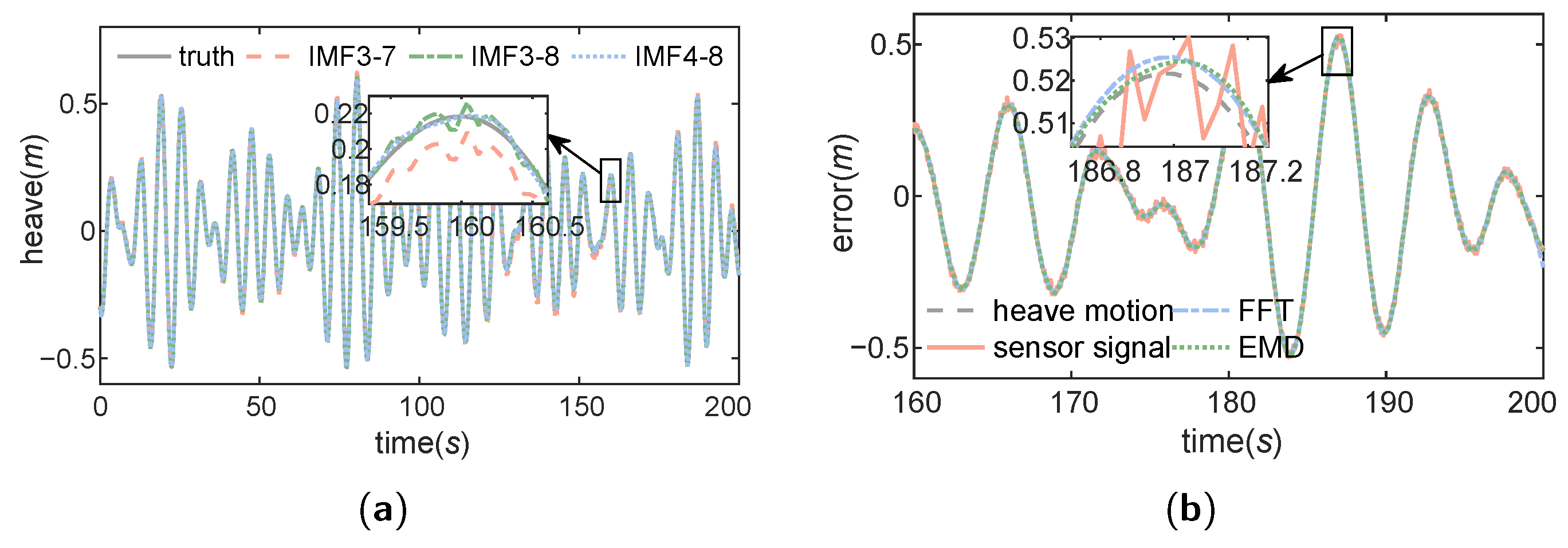
4.2. EMD Ablation Experiments

To identify the most suitable intrinsic mode functions (IMFs) for accurately recovering heave motion, i.e., to determine the values of p and q in Equation (20), this section compares the training results of various IMF groups. Further, to illustrate the necessity of EMD and its advantages in processing non-stationary ship motion signals with noise, this section compares the restoration results of heave motion by EMD and fast Fourier transform (FFT) [21].

The EMD results with different IMFs selected are shown in Figure 6a, and the training results are shown in

Table 4. The training errors with different IMFs selected.

	$\mathit{q}=3,\mathit{p}=7$	$\mathit{q}=2,\mathit{p}=8$	$\mathit{q}=3,\mathit{p}=8$
MAE (m)	0.01080	0.00303	0.00238
RMSE (m)	0.01253	0.00387	0.00304

. It can be seen that the training outputs exhibit the least error when $q=3, p=8$. This suggests that the training results with IMF4 to IMF8 selected are the most optimal. The output results of EMD and FFT are shown in Figure 6b. The results show that EMD provides superior restoration results of heave motion compared to FFT.

The training results without signal processing, after FFT processing and after EMD processing, are shown in

Table 5. The training errors without signal processing and with FFT or EMD processing.

	SBL	FFT-SBL	EMD-SBL
MAE (m)	0.00440	0.00334	0.00239
RMSE (m)	0.00553	0.00407	0.00307

. It can be seen that the output error of EMD is significantly smaller than FFT, indicating that EMD provides a superior restoration result of heave motion compared to FFT.

4.3. Training Results of the EMD-SBL-Based Heave Motion Prediction Model

To illustrate that SBL can determine the fewest terms required from past samples to avoid overfitting, this section shows the training results of the weights. The training weights are shown in

Table 6. Training weights of the EMD-SBL-based heave motion prediction model.

$w_1$	$w_2$	$w_3$	$w_4$	$w_5$	$w_6$
1.65985	−0.63717	0	−0.00170	0.00689	0.00272
$w_7$	$w_8$	$w_9$	$w_{10}$	$w_{11}$	$w_{12}$
−0.00125	0	0	−0.00792	0	−0.00653
$w_{13}$	$w_{14}$	$w_{15}$	$w_{16}$	$w_{17}$	$w_{18}$
−0.00794	−0.00526	0	−0.00550	0	0
$w_{19}$	$w_{20}$	$w_{21}$	$w_{22}$	$w_{23}$	$w_{24}$
0	−0.00352	0	0	0	0.00240

.

It can be observed that after introducing sparsity, the weights not contributing to the prediction are zero. The first two weights are the largest, while the subsequent weights are significantly smaller. It suggests that the future motion of the towing ship is significantly influenced by the motion observed in adjacent moments, with a gradual decline in distant points. This is because the sampling period of the sensor is relatively brief, and the sea condition generally remains consistent over the duration of a few sampling periods [29]. Therefore, incorporating recent samples is more effective in enhancing the accuracy of motion prediction compared to older samples.

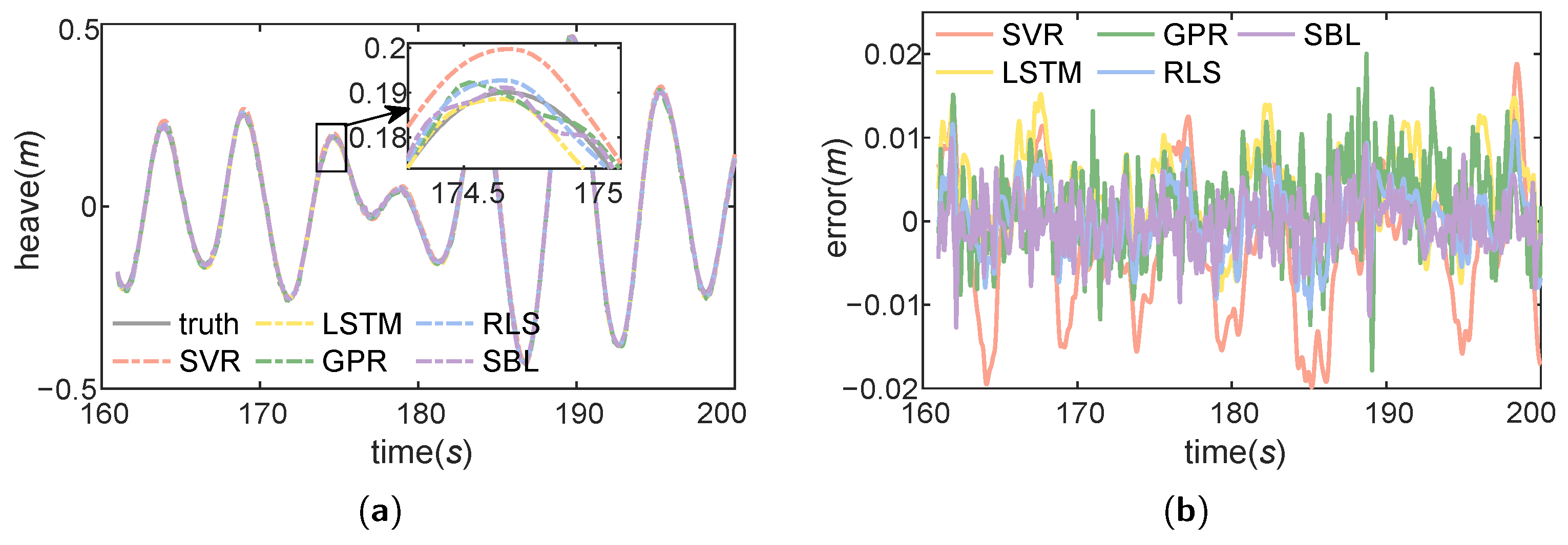
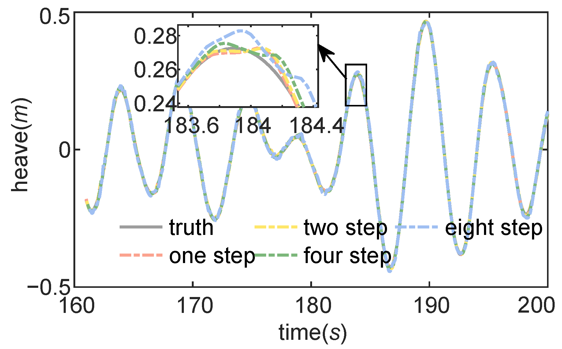
4.4. Heave Motion Prediction Experiments

Firstly, to illustrate the improved prediction accuracy, reliability and model adaptability after modeling, this section compares the prediction performance under different sea conditions of three data-based methods: (1) support vector regression (SVR) [13], (2) long short-term memory (LSTM) neural network [11], and (3) Gaussian process regression (GPR) [14] with two model-based methods—(1) recursive least square (RLS) [20] and (2) empirical mode decomposition-based sparse Bayesian learning (EMD-SBL). Subsequently, to demonstrate the superiority of EMD-SBL in parameter estimation, this section compares its prediction results with RLS. Finally, this section evaluates the performance of the EMD-SBL method in multi-step prediction to demonstrate its effectiveness over a short time horizon. Three metrics, i.e., mean absolute error (MAE), root mean square error (RMSE) and standard deviation (STD), are designed to evaluate the prediction performance.

The prediction results and prediction errors of the methods above with wind speed u = 7 m/s are shown in Figure 7. The MAE, RMSE and STD of the above methods with wind speed u = 7 m/s are shown in

Table 7. The evaluation of heave motion prediction.

Wind Speed	Evaluation	Data-Based Methods			Model-Based Methods
(m/s)	(m)	SVR	LSTM	GPR	RLS	SBL
	MAE	0.00694	0.00521	0.00425	0.00332	0.00252
u = 7 m/s	RMSE	0.00871	0.00643	0.00532	0.00408	0.00320
	STD	0.20007	0.19875	0.19848	0.19855	0.19795
	MAE	0.02299	0.01772	0.01429	0.00390	0.00258
u = 11 m/s	RMSE	0.03487	0.03277	0.02252	0.00498	0.00325
	STD	0.53159	0.52349	0.50551	0.51569	0.51690
	MAE	0.03108	0.02966	0.02583	0.00502	0.00267
u = 15 m/s	RMSE	0.03966	0.03800	0.03307	0.00594	0.00341
	STD	1.06264	1.05958	1.02100	1.04961	1.04642

. Simultaneously, to illustrate the improved reliability and model adaptability of the heave motion prediction after model developing, this section compares the prediction results of different methods above for the wind speeds u = 7, 11, 15 m/s. The results are shown in Table 7 and Figure 8. For comparison, the following prediction results are all obtained after the EMD process.

Table 7 shows that while the prediction dispersion of the algorithms is similar, the prediction errors vary significantly. The prediction errors of the three data-based methods (SVR, LSTM and GPR) are larger than the two model-based methods (RLS and SBL). Take wind speed u = 7 m/s as an example. The RLS, which exhibits the larger error among the two model-based methods, has an MAE of 78.1% and an RMSE of 76.7% relative to the GPR, which displays the smallest error among the three data-based methods. The results demonstrate that the prediction reliability is enhanced with the incorporation of additional model information. Among the two model-based methods, the prediction errors of SBL are less than RLS. The MAE of SBL is 75.9% of RLS, and the RMSE is 78.3% of RLS. It indicates that SBL has improved the prediction accuracy after introducing sparsity to avoid overfitting.

As shown in Table 7 and Figure 8, an increase in sea condition level leads to a corresponding rise in wave height, resulting in a larger amplitude of heave motion. Consequently, the prediction errors and the degree of data dispersion increase. However, the model-based methods demonstrate superior adaptability compared to the data-based methods with the increased sea condition level. Among the three data-based methods, LSTM does not demonstrate a substantial advantage over SVR due to the limited sample size. In contrast, GPR exhibits superior performance due to its advantages in the processing of small samples and nonlinear data. From u = 7 m/s to u = 15 m/s, the MAE of GPR increased by 508.3% and the RMSE increased by 522.0%, while the MAE of RLS only increased by 51.5% and the RMSE only increased by 45.7%. The prediction error of SBL, on the other hand, is barely affected, with its MAE and RMSE increasing by only 6.2% and 6.9%, respectively. It suggests that the model-based method demonstrates enhanced model adaptability in response to diverse sea conditions; among them, the advantages of SBL are particularly significant.

To illustrate that the EMD-SBL method can still maintain good prediction results in a short time, the prediction results of one, two, four and eight steps are compared as shown in Figure 9 and Figure 10 and

Table 8. The evaluation of one-step prediction and multi-step prediction.

k	1	2	4	8
MAE (m)	0.00252	0.00264	0.00330	0.00619
RMSE (m)	0.00320	0.00334	0.00410	0.00752

.

As observed from Figure 9 and Table 8, the prediction error increases with the prediction steps. However, the overall prediction accuracy remains at a level greater than 90%. It indicates that the EMD-SBL method can still have a good prediction effect in a short time.

4.5. Towed Vehicle Depth Compensation Experiments

Finally, this section compares the effects of towed vehicle depth compensation with and without prediction under various delay times to demonstrate the necessity of towing ship motion prediction for effective towed vehicle depth compensation. The compensation results with delays of 1, 2, 4 and 8 sampling periods are shown in Figure 10.

The results indicate that predictive compensation significantly outperforms non-predictive compensation, with the benefits of prediction becoming increasingly evident as the delay time increases. However, in practical applications, the marine environment and waves exhibit inherent randomness, introducing uncertainty into heave motion. The structure and parameters of the model may change over time, rendering offline-trained models ineffective. Therefore, how to shorten the training time and extend the prediction duration while ensuring prediction accuracy, so as to realize online learning or adaptive retraining, is crucial for real-world UTS deployment. These actual possible problems should also be discussed in a future study.

5. Conclusions

To improve the prediction effect of heave motion for the depth compensation of a towed vehicle, a simplified heave motion model under random waves is firstly developed based on the strip theory. Based on the model, an EMD-SBL algorithm is proposed for heave motion prediction. Furthermore, the depth of the towed vehicle is modeled and compensated according to the geometric relationship. Finally, through comparative experiments using classical data-based methods, including SVR, LSTM and GPR, as well as a model-based method, RLS, the proposed EMD-SBL method effectively reconstructs the heave motion from non-stationary sensor signals with noise, while introducing sparsity to prevent overfitting. This approach significantly improves both the prediction accuracy and model adaptability under various sea conditions, which demonstrates that the predicted depth compensation effect of the towed vehicle is significantly superior to that without prediction. For example, as the speed u changes from 7m/s to 15m/s, this corresponds to increases in the percentages of the MAE and RMSE with SVR, LSTM, GPR and RLS, which are almost (348%, 355%), (469%, 491%), (508%, 522%) and (56%, 46%), respectively. However, for the proposed EMD-SBL strategy, it displays decreases of almost (6%,6.6%), which shows that the model-based approach exhibits better model adaptability under various sea conditions, with the proposed EMD-SBL demonstrating particularly significant advantages.

However, in practical applications, the marine environment and waves exhibit inherent randomness, introducing uncertainty into heave motion. The structure and parameters of the model may change over time, rendering offline-trained models ineffective. Therefore, how to shorten the training time and extend the prediction duration while ensuring prediction accuracy, so as to realize online training, may be a problem that could be studied in the future.

References

1. Yang, X.; Wu, J.; Li, Q.; Lv, H. Numerical simulation of depth tracking control of an underwater towed system coupled with wave–ship interference. J. Mar. Sci. Eng. 2021, 9, 874. [Google Scholar] [CrossRef]
2. Wu, H.; Li, X.; Xu, K.; Song, D.; Xia, Y.; Xu, G. Motion Control of a Flexible-Towed Underwater Vehicle Based on Dual-Winch Differential Tension Coordination Control. J. Mar. Sci. Eng. 2025, 13, 1120. [Google Scholar] [CrossRef]
3. Woodacre, J.K.; Bauer, R.J.; Irani, R.A. A review of vertical motion heave compensation systems. Ocean. Eng. 2015, 104, 140–154. [Google Scholar] [CrossRef]
4. Tang, G.; Yao, X.; Li, F.; Wang, Y.; Hu, X. Prediction about the vessel’s heave motion under different sea states based on hybrid PSO-ARMA model. Ocean. Eng. 2022, 263, 112247. [Google Scholar] [CrossRef]
5. Majidian, H.; Enshaei, H.; Howe, D. Online short-term ship response prediction with dynamic buffer window using transient free switching filter. Ocean. Eng. 2024, 294, 116701. [Google Scholar] [CrossRef]
6. Jiang, H.; Duan, S.L.; Huang, L.M.; Han, Y.; Yang, H.; Ma, Q.W. Scale effects in AR model real-time ship motion prediction. Ocean. Eng. 2020, 203, 107202. [Google Scholar] [CrossRef]
7. Xu, D.W.; Wang, Y.D.; Jia, L.M.; Qin, Y.; Dong, H.H. Real-time road traffic state prediction based on ARIMA and Kalman filter. Front. Inf. Technol. Electron. Eng. 2017, 18, 287–302. [Google Scholar] [CrossRef]
8. Ge, Y.; Qin, M.J.; Niu, Q.T. Prediction of Ship Motion Attitude Based on BP Network. In Proceedings of the 2017 29th Chinese Control and Decision Conference (Ccdc), Chongqing, China, 28–30 May 2017; pp. 1596–1600. [Google Scholar] [CrossRef]
9. Li, Z.Y.; Dong, J.; Song, Z.K.; Zhang, H.C.; Guo, Y.B. Prediction of Ship Roll Motion Based on Combination of Phase Space Reconstruction Theory and Elman Network. In Proceedings of the 2016 IEEE International Conference on Information and Automation (ICIA), Ningbo, China, 31 July–4 August 2016; pp. 686–689. [Google Scholar] [CrossRef]
10. Yin, J.C.; Perakis, A.N.; Wang, N. A real-time ship roll motion prediction using wavelet transform and variable RBF network. Ocean. Eng. 2018, 160, 10–19. [Google Scholar] [CrossRef]
11. Tang, G.; Lei, J.M.; Shao, C.T.; Hu, X.; Cao, W.D.; Men, S.Y. Short-Term Prediction in Vessel Heave Motion Based on Improved LSTM Model. IEEE Access 2021, 9, 58067–58078. [Google Scholar] [CrossRef]
12. Tian, R.; Li, X.M.; Ma, Z.Y.; Liu, Y.X.; Wang, J.X.; Wang, C. LDformer: A parallel neural network model for long-term power forecasting. Front. Inf. Technol. Electron. Eng. 2023, 24, 1287–1301. [Google Scholar] [CrossRef]
13. Nie, Z.H.; Shen, F.; Xu, D.J.; Li, Q.H. An EMD-SVR model for short-term prediction of ship motion using mirror symmetry and SVR algorithms to eliminate EMD boundary effect. Ocean. Eng. 2020, 217, 107927. [Google Scholar] [CrossRef]
14. Ouyang, Z.L.; Zou, Z.J. Nonparametric modeling of ship maneuvering motion based on Gaussian process regression optimized by genetic algorithm. Ocean. Eng. 2021, 238, 109699. [Google Scholar] [CrossRef]
15. Amini-Afshar, M.; Bingham, H.B. Added resistance using Salvesen-Tuck-Faltinsen strip theory and the Kochin function. Appl. Ocean. Res. 2021, 106, 102481. [Google Scholar] [CrossRef]
16. Chen, J.P.; Zhu, D.X. Numerical Simulations of Wave-Induced Ship Motions in Time Domain by a Rankine Panel Method. J. Hydrodyn. 2010, 22, 373–380. [Google Scholar] [CrossRef]
17. Zhang, P.; Zhang, T.; Wang, X. Hydrodynamic Analysis and Motions of Ship with Forward Speed via a Three-Dimensional Time-Domain Panel Method. J. Mar. Sci. Eng. 2021, 9, 87. [Google Scholar] [CrossRef]
18. Tang, K.; Wang, J.X.; Chen, X.; Jiang, D.P.; Li, Y.L. Nonlinear ship motion with forward speed in waves based on 3D time domain hybrid Green function method. Eng. Anal. Bound. Elem. 2021, 123, 107–121. [Google Scholar] [CrossRef]
19. Gadelho, J.F.M.; Rodrigues, J.M.; Lavrov, A.; Soares, C.G. Heave and sway hydrodynamic coefficients of ship hull sections in deep and shallow water using Navier-Stokes equations. Ocean. Eng. 2018, 154, 262–276. [Google Scholar] [CrossRef]
20. Richter, M.; Schaut, S.; Walser, D.; Schneider, K.; Sawodny, O. Experimental validation of an active heave compensation system: Estimation, prediction and control. Control Eng. Pract. 2017, 66, 1–12. [Google Scholar] [CrossRef]
21. Küchler, S.; Mahl, T.; Neupert, J.; Schneider, K.; Sawodny, O. Active Control for an Offshore Crane Using Prediction of the Vessel’s Motion. IEEE/ASME Trans. Mechatronics 2011, 16, 297–309. [Google Scholar] [CrossRef]
22. Xia, D.W.; Geng, J.; Huang, R.X.; Shen, B.Q.; Hu, Y.; Li, Y.T.; Li, H.Q. A distributed EEMDN-SABiGRU model on Spark for passenger hotspot prediction. Front. Inf. Technol. Electron. Eng. 2023, 24, 1316–1331. [Google Scholar] [CrossRef]
23. Brunton, S.L.; Proctor, J.L.; Kutz, J.N. Discovering governing equations from data by sparse identification of nonlinear dynamical systems. Proc. Natl. Acad. Sci. USA 2016, 113, 3932–3937. [Google Scholar] [CrossRef]
24. Calnan, C.; Bauer, R.J.; Irani, R.A. Reference-Point Algorithms for Active Motion Compensation of Towed Bodies. IEEE J. Ocean. Eng. 2019, 44, 1024–1040. [Google Scholar] [CrossRef]
25. Vegte, J.V.D. Fundamentals of Digital Signal Processing; Publishing House of Electronics Industry: Beijing, China, 2003; pp. 293–298. [Google Scholar]
26. Huang, N.E.; Shen, Z.; Long, S.R.; Wu, M.L.C.; Shih, H.H.; Zheng, Q.N.; Yen, N.C.; Tung, C.C.; Liu, H.H. The empirical mode decomposition and the Hilbert spectrum for nonlinear and non-stationary time series analysis. Proc. R. Soc. A Math. Phys. Eng. Sci. 1998, 454, 903–995. [Google Scholar] [CrossRef]
27. Tipping, M.E. Sparse Bayesian learning and the relevance vector machine. J. Mach. Learn. Res. 2001, 1, 211–244. [Google Scholar] [CrossRef]
28. Pierson, W.J., Jr.; Moskowitz, L. A proposed spectral form for fully developed wind seas based on the similarity theory of SA Kitaigorodskii. J. Geophys. Res. 1964, 69, 5181–5190. [Google Scholar] [CrossRef]
29. Xu, C.Z.; Zou, Z.J. Online Prediction of Ship Roll Motion in Waves Based on Auto-Moving Gird Search-Least Square Support Vector Machine. Math. Probl. Eng. 2021, 2021, 2760517. [Google Scholar] [CrossRef]
Figure 1. The typical underwater towed system used for shallow water exploration.
Jmse 13 01427 g001
Figure 2. System model.
Jmse 13 01427 g002
Figure 3. The depth model of a towed vehicle based on the heave motion of the towing ship.
Jmse 13 01427 g003
Figure 4. Heave motion prediction model.
Jmse 13 01427 g004
Figure 5. Schematic diagram of heave motion prediction using EMD-SBL.
Jmse 13 01427 g005
Figure 6. The EMD results with different IMFs selected (a), and the heave motion restoration results with EMD (b).
Jmse 13 01427 g006
Figure 7. The heave motion prediction results (a) and errors (b) of different methods with wind speed u = 7 m/s.
Jmse 13 01427 g007
Figure 8. The MAE (a) and RMSE (b) of heave motion prediction with wind speed u = 7, 11, 15 m/s.
Jmse 13 01427 g008
Figure 9. The results of one-step prediction and multi-step prediction.
Jmse 13 01427 g009
Figure 10. The depth compensation results of a towed vehicle with delays of 1 (a), 2 (b), 4 (c), and 8 (d) sampling periods.
Jmse 13 01427 g010