
STNet: Prediction of Underwater Sound Speed Profiles with an Advanced Semi-Transformer Neural Network


Abstract
1. Introduction
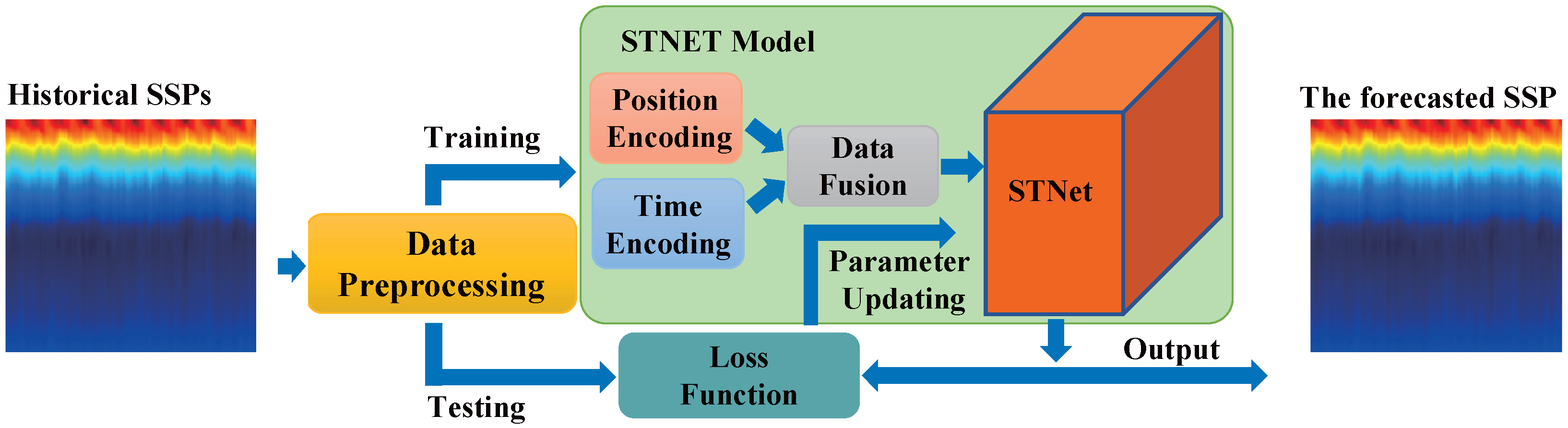
- To achieve accurate and real-time long-term prediction of ocean SSPs without on-site data measurements, we propose the STNet model for SSP prediction, which overcomes the prolonged training time associated with complex encoder–decoder structures in traditional transformers.
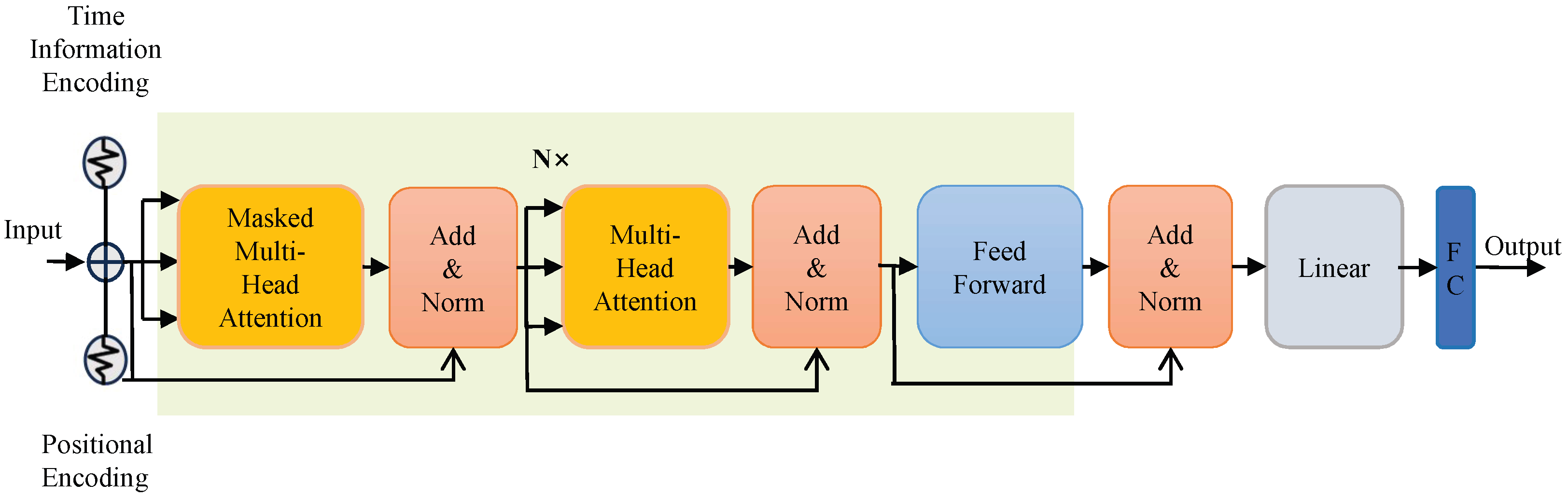
- To improve execution efficiency, we propose a parallel processing strategy for the training process of the STNet model. Time encoding and position encoding are sequentially applied to the sound velocity data to form a spatiotemporal distribution data matrix. Then, the attention mechanism is used to capture the inherent dependency relationship between the temporal dynamics and spatial distribution of the data.
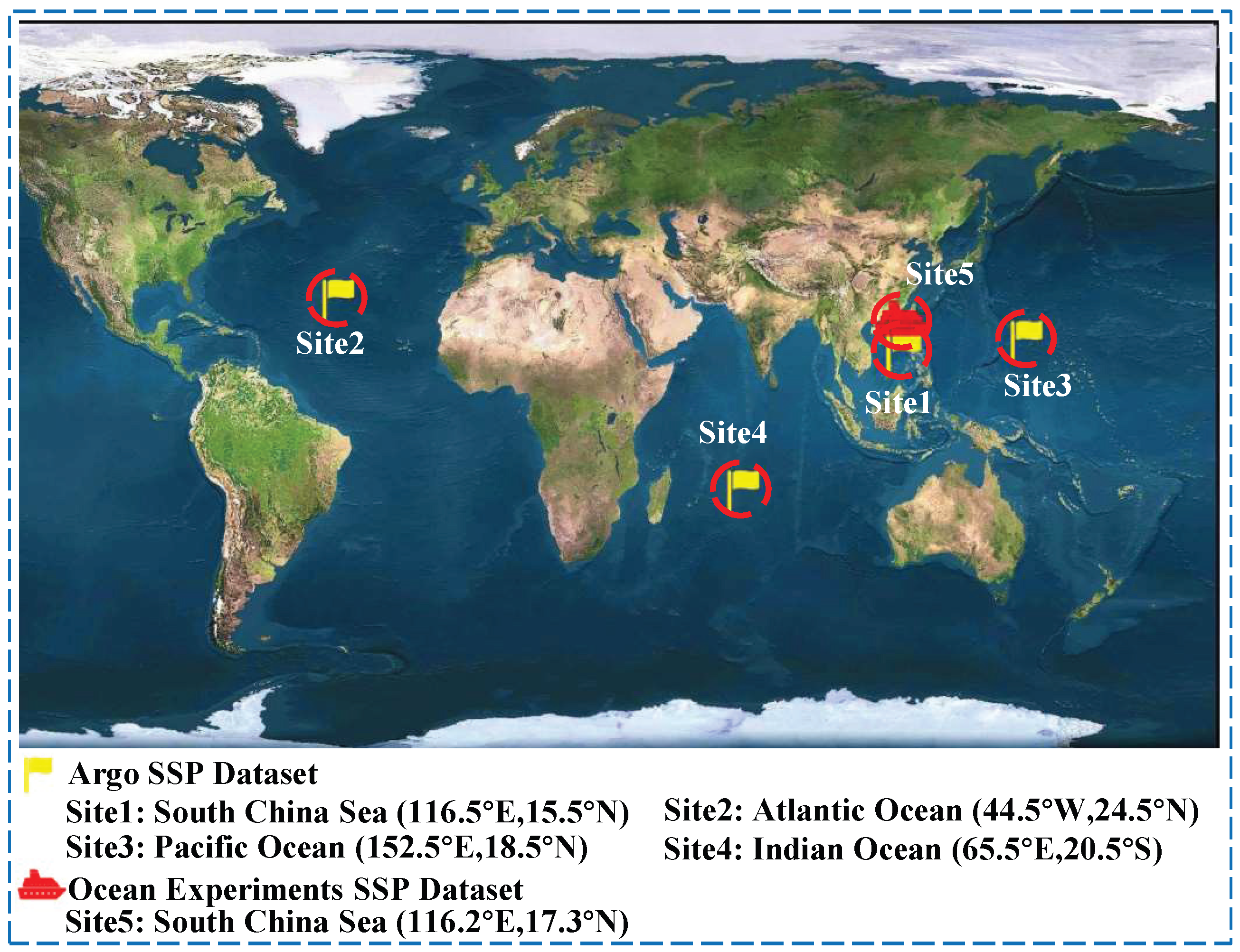
- To fully evaluate the effectiveness of STNet, we tested the model using historical long-period Argo observation data and short-period experimental data measured from the South China Sea in April 2023. The experimental results indicated that STNet exhibited superior performance in predicting both long- and short-period sound velocity distributions.
2. Related Works
3. Methodology
3.1. Overall Framework for SSP Prediction
3.2. Data and Preprocessing
3.2.1. Data Source
3.2.2. Data Resampling
3.3. STNet Model
3.3.1. Time Encoding
3.3.2. Positional Encoding
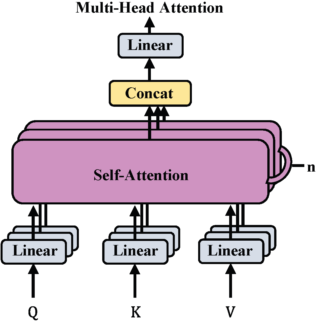
3.3.3. Self-Attention Mechanism
Multi-Head Attention Mechanism
Masked Multi-Head Attention Mechanism
3.3.4. Feed-Forward Neural Network Layer
3.3.5. Model Parameter Updating
4. Results and Discussions
4.1. Parameter Settings and Baselines
4.2. Influence of Training Time Stepping
4.3. Influence of Training Data Length
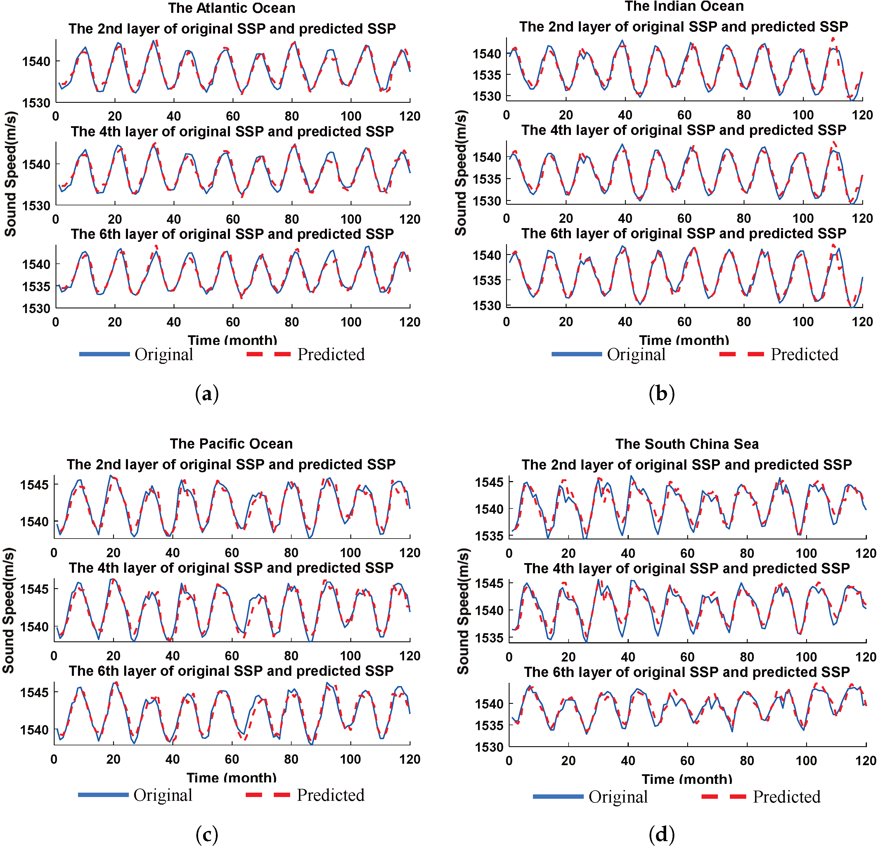
4.4. Evaluation of Periodic Capture Capability
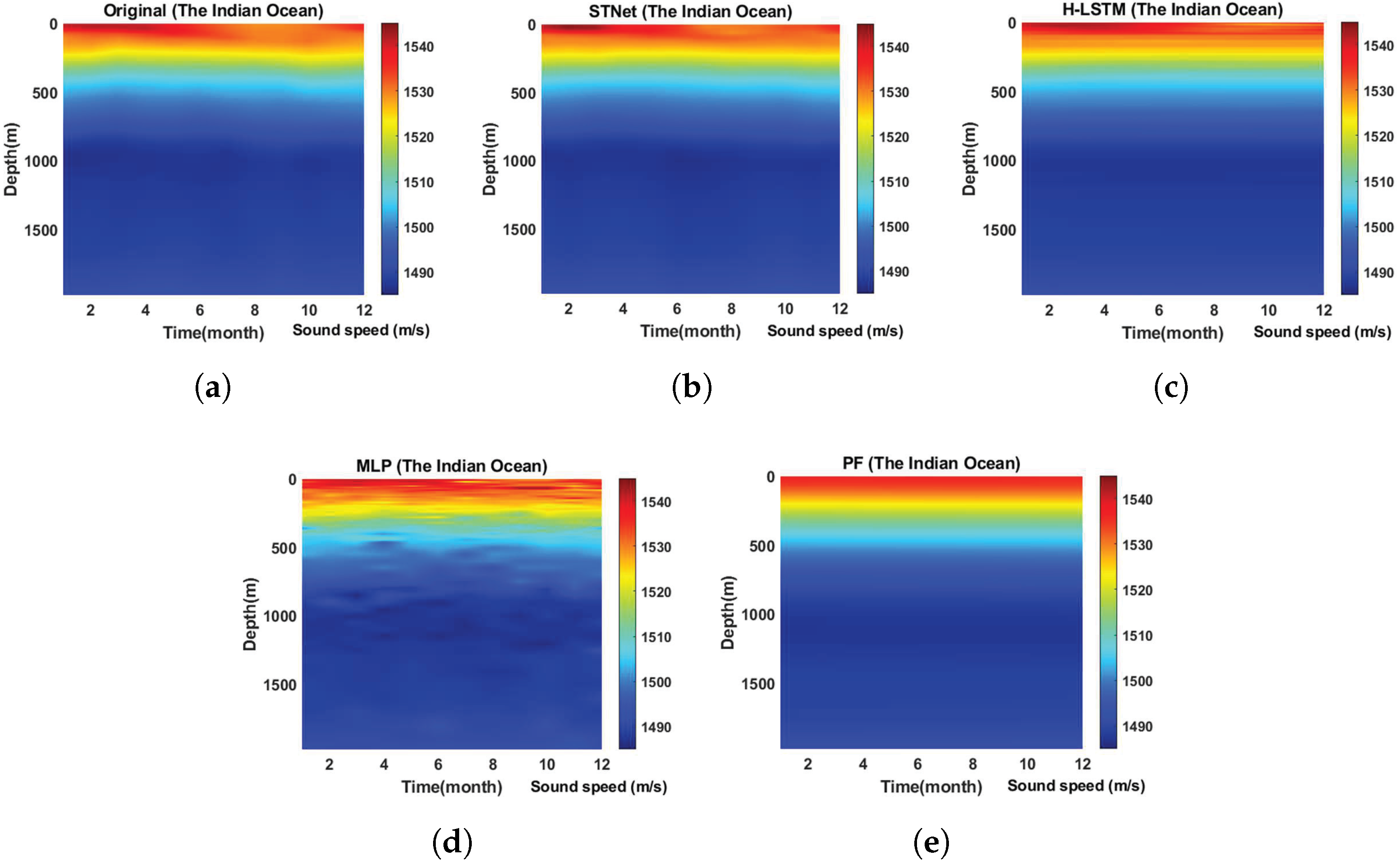
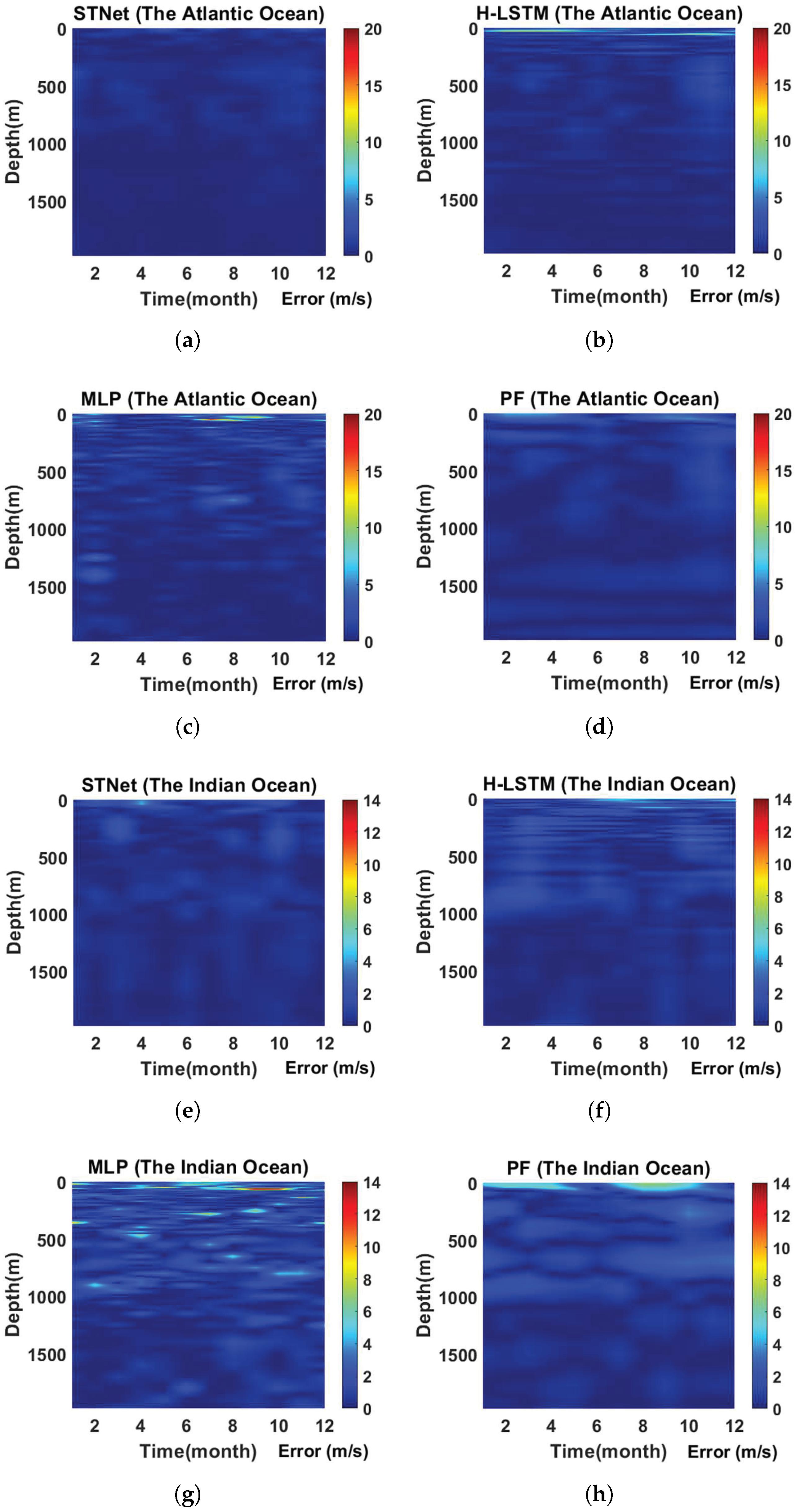
4.5. Long-Term Predictive Performance Evaluation
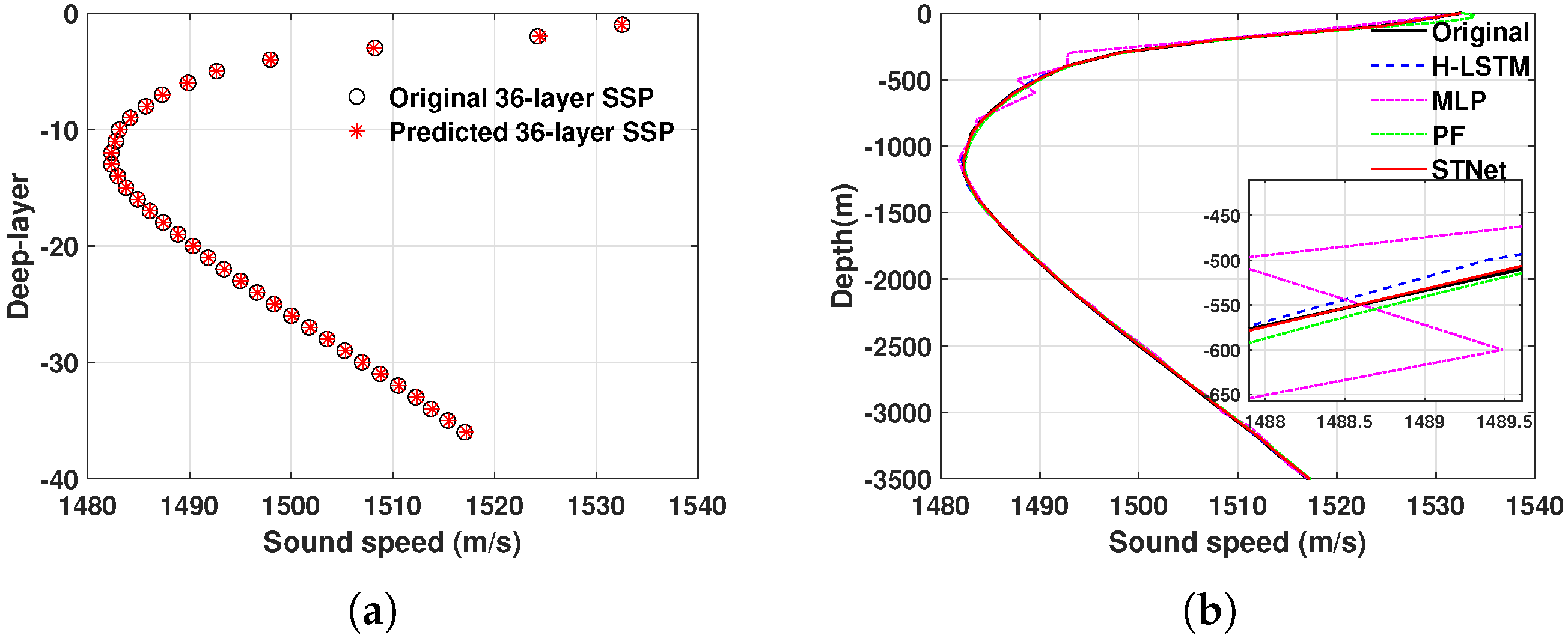
4.6. Short-Term Predictive Performance Evaluation
4.7. Comparison of Execution Efficiency
5. Conclusions
Author Contributions
Funding
Data Availability Statement
Conflicts of Interest
Abbreviations
| SSP | Sound speed profile |
| STNet | Semi-transformer neural network |
| MFP | Matched field processing |
| CS | Compressed sensing |
| GA | Genetic algorithm |
References
- Huang, W.; Wu, P.; Lu, J.; Lu, J.; Xiu, Z.; Xu, Z.; Li, S.; Xu, T. Underwater SSP Measurement and Estimation: A Survey. J. Mar. Sci. Eng. 2024, 12, 2356. [Google Scholar] [CrossRef]
- Erol-Kantarci, M.; Mouftah, H.T.; Oktug, S. A Survey of Architectures and Localization Techniques for Underwater Acoustic Sensor Networks. IEEE Commun. Surv. Tutor. 2011, 13, 487–502. [Google Scholar] [CrossRef]
- Luo, J.; Yang, Y.; Wang, Z.; Chen, Y. Localization Algorithm for Underwater Sensor Network: A Review. IEEE Internet Things J. 2021, 8, 13126–13144. [Google Scholar] [CrossRef]
- Liu, Y.; Wang, Y.; Chen, C.; Liu, C. Unified Underwater Acoustic Localization and Sound Speed Estimation for an Isogradient Sound Speed Profile. IEEE Sens. J. 2024, 24, 3317–3327. [Google Scholar] [CrossRef]
- Munk, W.; Wunsch, C. Ocean acoustic tomography: Rays and modes. Rev. Geophys. 1983, 21, 777–793. [Google Scholar] [CrossRef]
- Jensen, F.B.; Kuperman, W.A.; Porter, M.B.; Schmidt, H. Computational Ocean Acoustics: Chapter 1; Springer Science & Business Media: Berlin/Heidelberg, Germany, 2011; pp. 3–4. [Google Scholar] [CrossRef]
- Liu, B.; Tang, X.; Tharmarasa, R.; Kirubarajan, T.; Jassemi, R.; Hallé, S. Underwater Target Tracking in Uncertain Multipath Ocean Environments. IEEE Trans. Aerosp. Electron. Syst. 2020, 56, 4899–4915. [Google Scholar] [CrossRef]
- Zhang, S.; Xu, X.; Xu, D.; Long, K.; Shen, C.; Tian, C. The design and calibration of a low-cost underwater sound velocity profiler. Front. Mar. Sci. 2022, 9, 996299. [Google Scholar] [CrossRef]
- Luo, C.; Wang, Y.; Wang, C.; Yang, M.; Yang, S. Analysis of Glider Motion Effects on Pumped CTD. In Proceedings of the OCEANS 2023, Limerick, Ireland, 5–8 June 2023; pp. 1–7. [Google Scholar] [CrossRef]
- Kirimoto, K.; Han, J.; Konashi, S. Development of High Accuracy CTD Sensor: 5EL-CTD. In Proceedings of the OCEANS 2024, Singapore, 14–18 April 2024; pp. 1–8. [Google Scholar] [CrossRef]
- Tolstoy, A.; Diachok, O.; Frazer, L.N. Acoustic tomography via matched field processing. J. Acoust. Soc. Am. 1991, 89, 1119–1127. [Google Scholar] [CrossRef]
- Choo, Y.; Seong, W. Compressive Sound Speed Profile Inversion Using Beamforming Results. Remote Sens. 2018, 10, 704. [Google Scholar] [CrossRef]
- Bianco, M.; Gerstoft, P. Dictionary learning of sound speed profiles. J. Acoust. Soc. Am. 2017, 141, 1749–1758. [Google Scholar] [CrossRef] [PubMed]
- Huang, W.; Liu, M.; Li, D.; Yin, F.; Chen, H.; Zhou, J.; Xu, H. Collaborating Ray Tracing and AI Model for AUV-Assisted 3-D Underwater Sound-Speed Inversion. IEEE J. Ocean. Eng. 2021, 46, 1372–1390. [Google Scholar] [CrossRef]
- Piao, S.; Yan, X.; Li, Q.; Li, Z.; Wang, Z.; Zhu, J. Time series prediction of shallow water sound speed profile in the presence of internal solitary wave trains. Ocean Eng. 2023, 283, 115058. [Google Scholar] [CrossRef]
- Vaswani, A.; Shazeer, N.; Parmar, N.; Uszkoreit, J.; Jones, L.; Gomez, A.N.; Kaiser, L.; Polosukhin, I. Attention is all you need. In Proceedings of the 31st International Conference on Neural Information Processing Systems, Red Hook, NY, USA, 4–9 December 2017; NIPS’17. pp. 6000–6010. [Google Scholar]
- Munk, W.; Wunsch, C. Ocean acoustic tomography: A scheme for large scale monitoring. Deep-Sea Res. Part I-Oceanogr. Res. Pap. 1979, 26, 123–161. [Google Scholar] [CrossRef]
- Taroudakis, M.I.; Markaki, M.G. Matched Field Ocean Acoustic Tomography Using Genetic Algorithms. In Acoustical Imaging; Tortoli, P., Masotti, L., Eds.; Springer: Boston, MA, USA, 1996; pp. 601–606. [Google Scholar] [CrossRef]
- Yu, Y.; Li, Z.; He, L. Matched-field inversion of sound speed profile in shallow water using a parallel genetic algorithm. Chin. J. Oceanol. Limnol. 2010, 28, 1080–1085. [Google Scholar] [CrossRef]
- Bianco, M.J.; Gerstoft, P.; Traer, J.; Ozanich, E.; Roch, M.A.; Gannot, S.; Deledalle, C.A. Machine learning in acoustics: Theory and applications. J. Acoust. Soc. Am. 2019, 146, 3590–3628. [Google Scholar] [CrossRef] [PubMed]
- Reichstein, M.; Camps-Valls, G.; Stevens, B.; Jung, M.; Denzler, J.; Carvalhais, N.; Prabhat, F. Deep learning and process understanding for data-driven Earth system science. Nature 2019, 566, 195–204. [Google Scholar] [CrossRef] [PubMed]
- Jain, S.; Ali, M. Estimation of Sound Speed Profiles Using Artificial Neural Networks. IEEE Geosci. Remote Sens. Lett. 2006, 3, 467–470. [Google Scholar] [CrossRef]
- Li, H.; Qu, K.; Zhou, J. Reconstructing Sound Speed Profile From Remote Sensing Data: Nonlinear Inversion Based on Self-Organizing Map. IEEE Access 2021, 9, 109754–109762. [Google Scholar] [CrossRef]
- Ou, Z.; Qu, K.; Shi, M.; Wang, Y.; Zhou, J. Estimation of sound speed profiles based on remote sensing parameters using a scalable end-to-end tree boosting model. Front. Mar. Sci. 2022, 9, 1051820. [Google Scholar] [CrossRef]
- Yu, X.; Xu, T.; Wang, J. Sound Velocity Profile Prediction Method Based on RBF Neural Network. In China Satellite Navigation Conference (CSNC) 2020 Proceedings: Volume III; Springer: Singapore, 2020; pp. 475–487. [Google Scholar]
- Liu, Y.; Chen, Y.; Meng, Z.; Chen, W. Performance of single empirical orthogonal function regression method in global sound speed profile inversion and sound field prediction. Appl. Ocean Res. 2023, 136, 103598. [Google Scholar] [CrossRef]
- Kim, Y.J.; Han, D.; Jang, E.; Im, J.; Sung, T. Remote sensing of sea surface salinity: Challenges and research directions. GISci. Remote Sens. 2023, 60, 2166377. [Google Scholar] [CrossRef]
- Lu, J.; Huang, W.; Zhang, H. Dynamic Prediction of Full-Ocean Depth SSP by a Hierarchical LSTM: An Experimental Result. IEEE Geosci. Remote Sens. Lett. 2024, 21, 1–5. [Google Scholar] [CrossRef]
- Xie, C.; Miaomiao, X.; Cao, S.; Zhang, Y.; Zhang, C. Gridded Argo data set based on GDCSM analysis technique: Establishment and preliminary applications. J. Mar. Sci. 2019, 37, 24–35. [Google Scholar]
- Huang, W.; Lu, J.; Li, S.; Xu, T.; Wang, J.; Zhang, H. Fast Estimation of Full Depth Sound Speed Profile Based on Partial Prior Information. In Proceedings of the 2023 IEEE 6th International Conference on Electronic Information and Communication Technology (ICEICT), Qingdao, China, 21–24 July 2023; pp. 479–484. [Google Scholar] [CrossRef]
- Liu, F.; Ji, T.; Zhang, Q. Sound Speed Profile Inversion Based on Mode Signal and Polynomial Fitting. Acta Armamentarii 2019, 40, 2283–2295. [Google Scholar] [CrossRef]


| GDCSM_Argo Data | |||||
| Area | Time Dimension | Temporal Resolution | Number of SSPs | Depth | Layers |
| South China Sea ( E, N) | 2013–2022 (120 months) | one month | 120 | 0–1975 m | unequal interval (58 layers) |
| Atlantic Ocean ( W, N) | |||||
| Pacific Ocean ( E, N) | |||||
| Indian Ocean ( E, S) | |||||
| SCS-SSP Data | |||||
| South China Sea ( E, N) | 12–14 April 2023 | Around 2 h | 14 | 0–3500 m | equal interval (36 layers) |
| Parameter | Setting |
|---|---|
| Dimension of sequence input layer | 58/36 |
| Number of heads | 8 |
| Number of attention channels | 4 |
| Neurons of FNN layer | 128 |
| Dropout rate | 0.15 |
| Max epoch | 300 |
| Batch size | 32 |
| Optimizer | Adam |
| Initial learning rate | 0.001 |
| Training Time Step/Month | RMSE for Different Months (m/s) | Average RMSE (m/s) | |||||||||||
|---|---|---|---|---|---|---|---|---|---|---|---|---|---|
| 1 | 2 | 3 | 4 | 5 | 6 | 7 | 8 | 9 | 10 | 11 | 12 | ||
| 1 time step | 0.637 | 0.563 | 0.751 | 0.405 | 0.445 | 0.983 | 0.444 | 0.675 | 0.422 | 0.813 | 0.529 | 0.309 | 0.581 |
| 2 time steps | 0.602 | 0.546 | 0.808 | 0.534 | 0.784 | 0.965 | 0.904 | 0.950 | 0.350 | 0.923 | 1.307 | 0.495 | 0.763 |
| 4 time steps | 0.776 | 0.478 | 0.468 | 0.653 | 1.270 | 1.338 | 0.485 | 0.930 | 0.536 | 0.662 | 0.998 | 0.577 | 0.764 |
| 6 time steps | 0.705 | 0.706 | 0.800 | 0.851 | 0.557 | 0.846 | 0.784 | 0.827 | 0.752 | 1.040 | 1.132 | 0.470 | 0.789 |
| 10 time steps | 0.996 | 1.241 | 1.357 | 1.253 | 0.731 | 0.848 | 0.455 | 0.662 | 0.569 | 0.702 | 0.663 | 0.584 | 0.838 |
| Training Data Length/Month | RMSE for Different Months (m/s) | Average RMSE (m/s) | |||||||||||
|---|---|---|---|---|---|---|---|---|---|---|---|---|---|
| 1 | 2 | 3 | 4 | 5 | 6 | 7 | 8 | 9 | 10 | 11 | 12 | ||
| 1 year | 1.647 | 0.529 | 0.805 | 0.795 | 0.858 | 0.813 | 1.175 | 1.041 | 0.880 | 0.949 | 0.857 | 0.816 | 0.930 |
| 3 years | 0.521 | 0.678 | 1.320 | 0.584 | 0.980 | 1.288 | 0.781 | 0.711 | 0.779 | 0.767 | 0.739 | 0.837 | 0.832 |
| 5 years | 0.667 | 0.755 | 0.934 | 0.854 | 0.556 | 1.057 | 0.621 | 0.405 | 0.548 | 0.550 | 0.432 | 0.583 | 0.664 |
| 7 years | 0.698 | 0.537 | 0.557 | 0.689 | 0.465 | 1.023 | 0.629 | 0.601 | 0.373 | 0.453 | 0.487 | 0.549 | 0.588 |
| 9 years | 0.637 | 0.563 | 0.751 | 0.405 | 0.445 | 0.983 | 0.444 | 0.675 | 0.422 | 0.813 | 0.529 | 0.309 | 0.581 |
| Method | STNet | H-LSTM | MLP | PF |
|---|---|---|---|---|
| RMSE (m/s) | 0.079 | 0.153 | 0.957 | 0.548 |
| Method | STNet | H-LSTM | MLP | PF |
|---|---|---|---|---|
| Training time (s) | 28.07 | 223.19 | 232.30 | 12.33 |
Disclaimer/Publisher’s Note: The statements, opinions and data contained in all publications are solely those of the individual author(s) and contributor(s) and not of MDPI and/or the editor(s). MDPI and/or the editor(s) disclaim responsibility for any injury to people or property resulting from any ideas, methods, instructions or products referred to in the content. |
© 2025 by the authors. Licensee MDPI, Basel, Switzerland. This article is an open access article distributed under the terms and conditions of the Creative Commons Attribution (CC BY) license (https://creativecommons.org/licenses/by/4.0/).
Share and Cite
Huang, W.; Lu, J.; Lu, J.; Wu, Y.; Zhang, H.; Xu, T. STNet: Prediction of Underwater Sound Speed Profiles with an Advanced Semi-Transformer Neural Network. J. Mar. Sci. Eng. 2025, 13, 1370. https://doi.org/10.3390/jmse13071370
Huang W, Lu J, Lu J, Wu Y, Zhang H, Xu T. STNet: Prediction of Underwater Sound Speed Profiles with an Advanced Semi-Transformer Neural Network. Journal of Marine Science and Engineering. 2025; 13(7):1370. https://doi.org/10.3390/jmse13071370
Chicago/Turabian StyleHuang, Wei, Junpeng Lu, Jiajun Lu, Yanan Wu, Hao Zhang, and Tianhe Xu. 2025. "STNet: Prediction of Underwater Sound Speed Profiles with an Advanced Semi-Transformer Neural Network" Journal of Marine Science and Engineering 13, no. 7: 1370. https://doi.org/10.3390/jmse13071370
APA StyleHuang, W., Lu, J., Lu, J., Wu, Y., Zhang, H., & Xu, T. (2025). STNet: Prediction of Underwater Sound Speed Profiles with an Advanced Semi-Transformer Neural Network. Journal of Marine Science and Engineering, 13(7), 1370. https://doi.org/10.3390/jmse13071370