

A Mainlobe Interference Suppression Method for Small Hydrophone Arrays


Abstract
1. Introduction
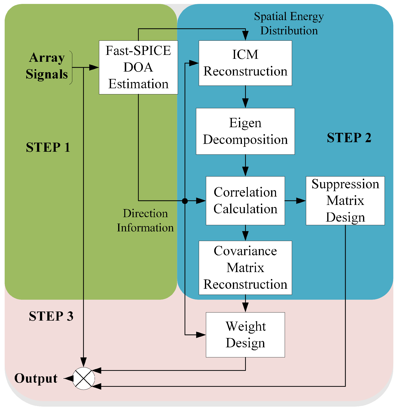
2. Methods
2.1. Signal Model
2.2. Improved DOA Estimation Method
2.3. Interference Suppression Weight
3. Simulations
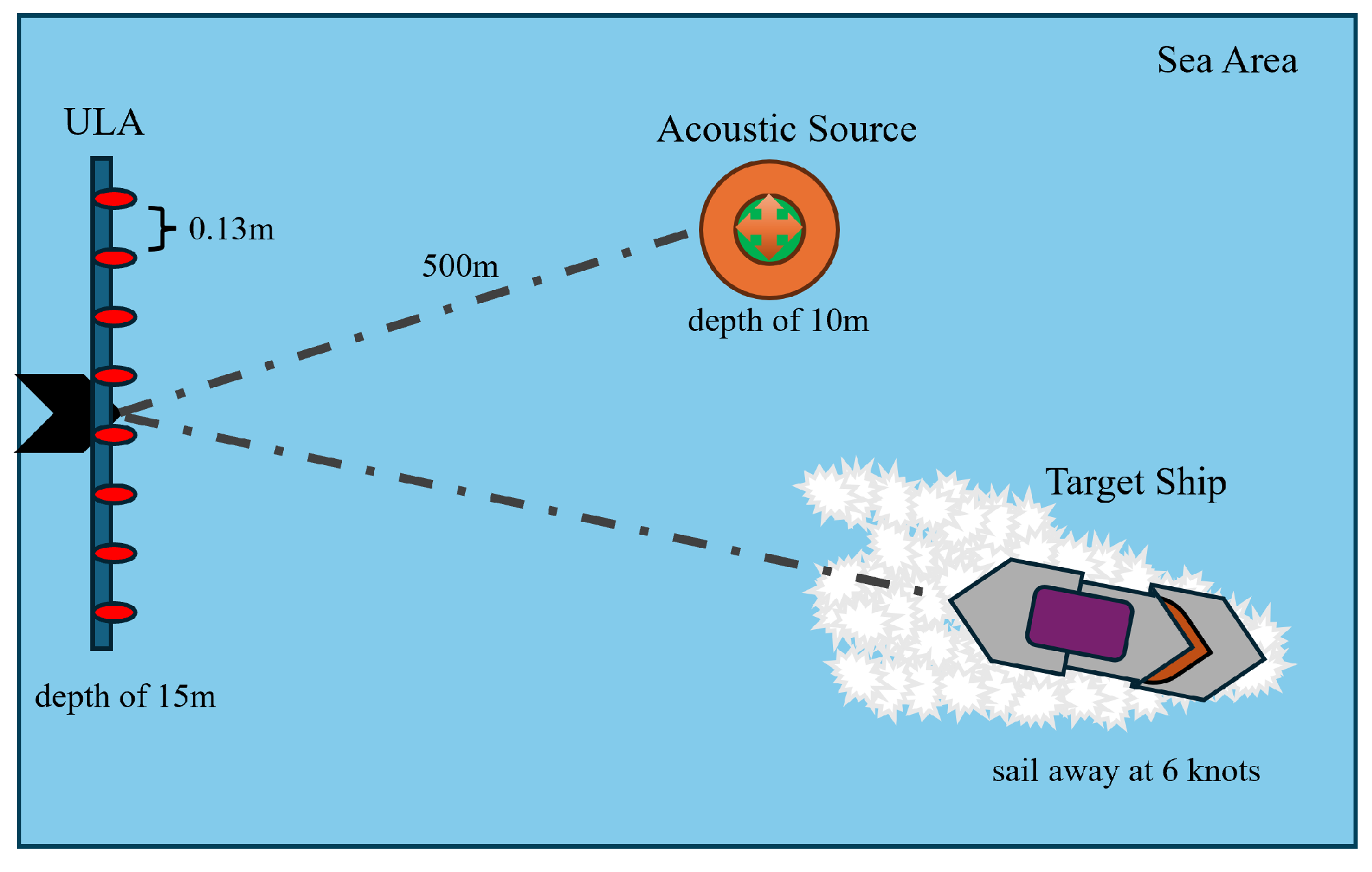
3.1. Simulation Setup
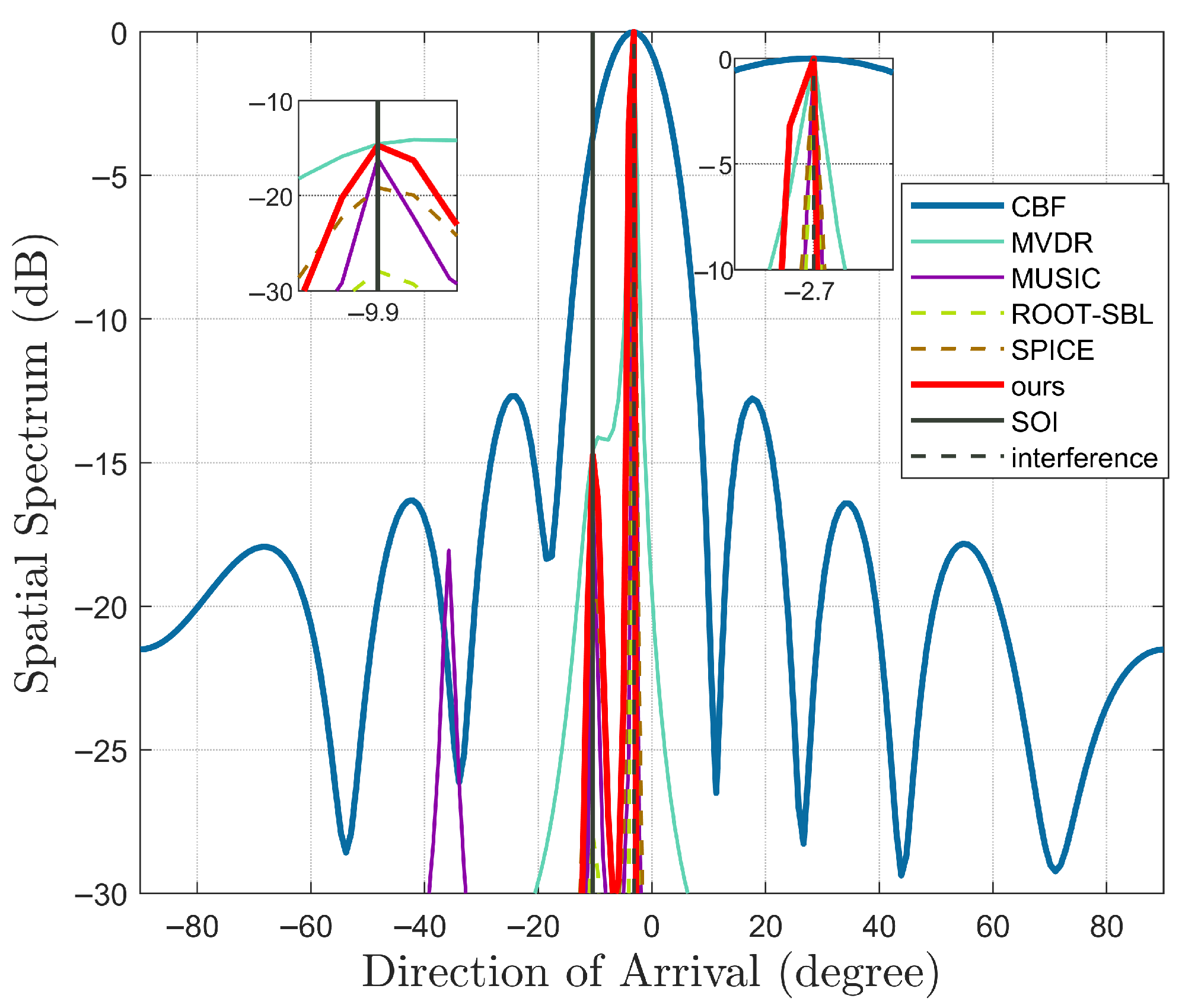
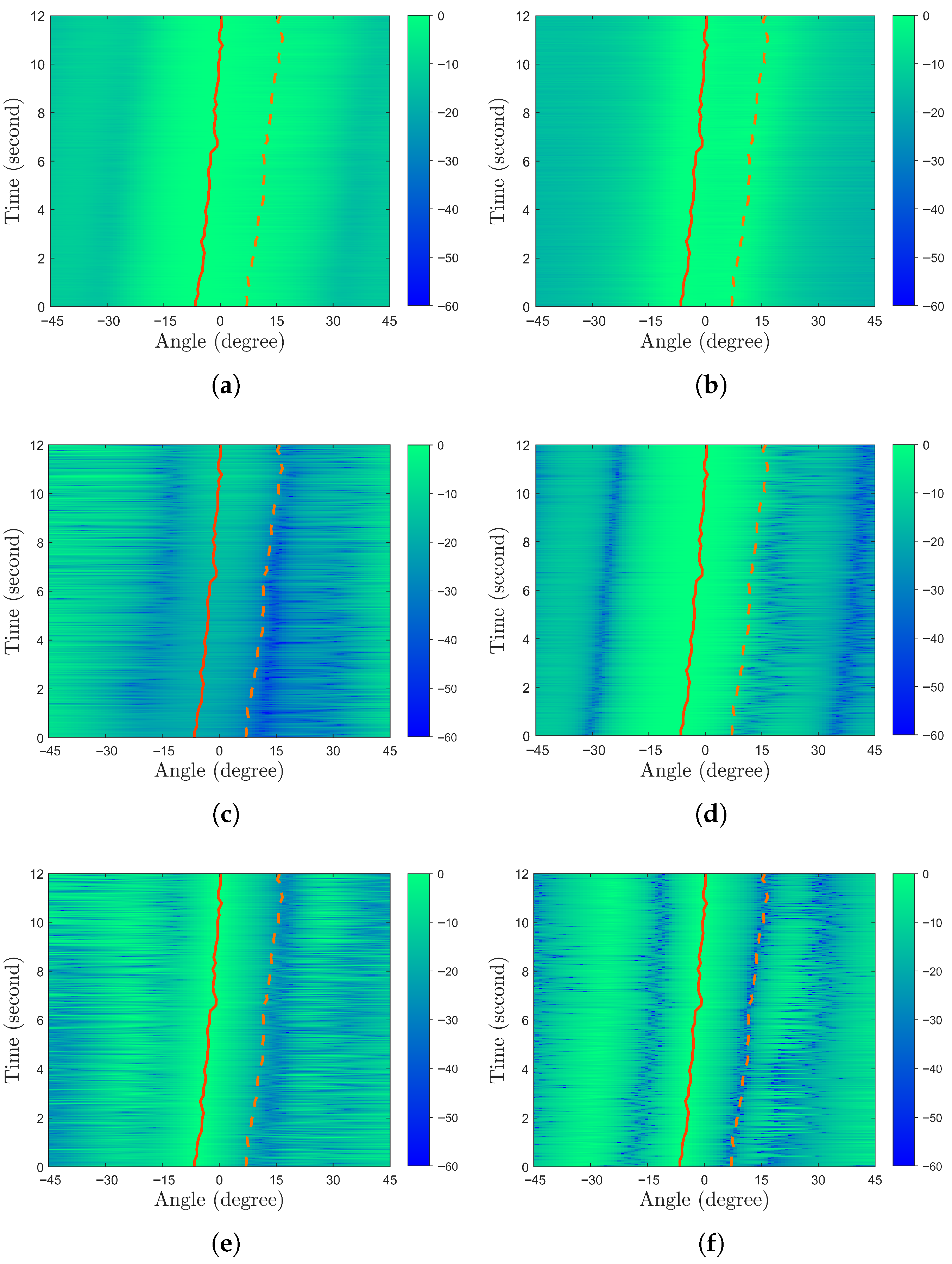
3.2. DOA Estimation Simulation
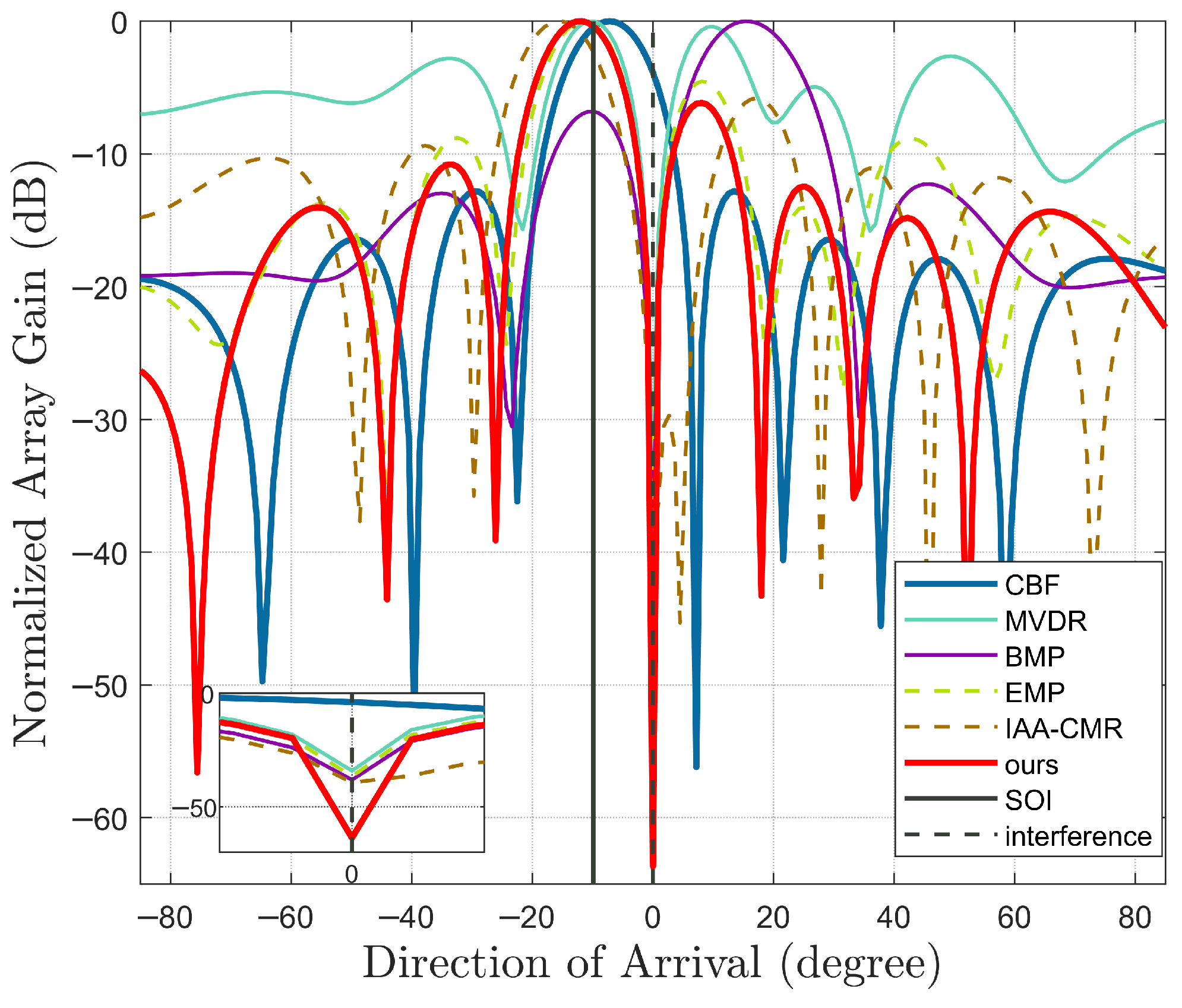
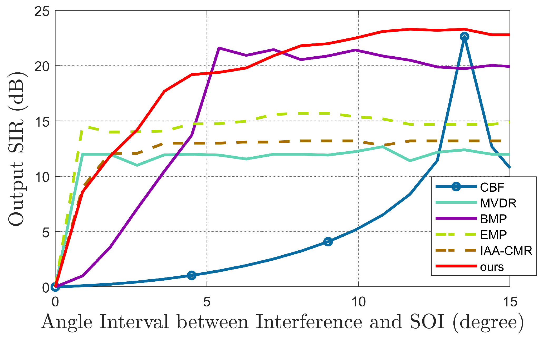
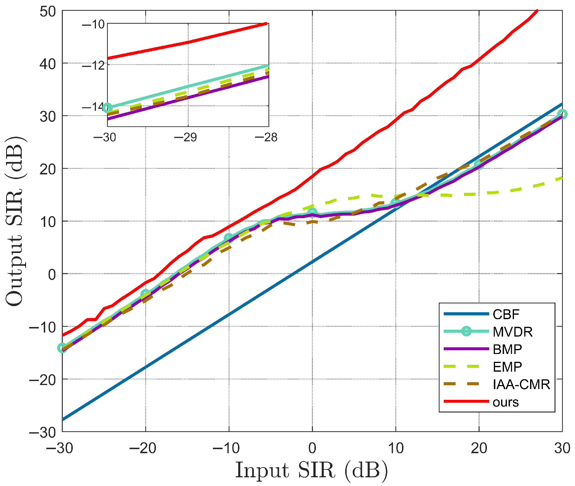
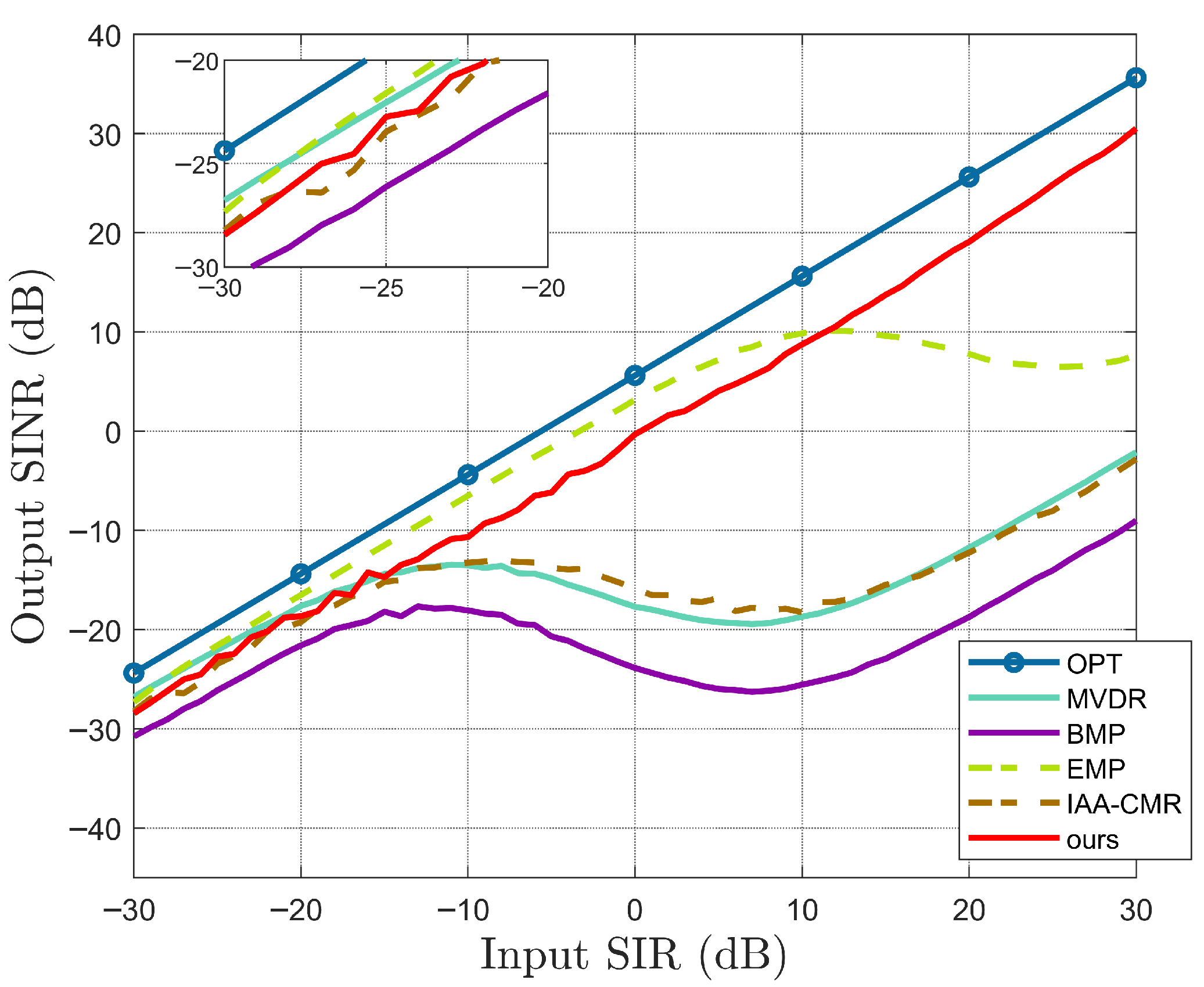
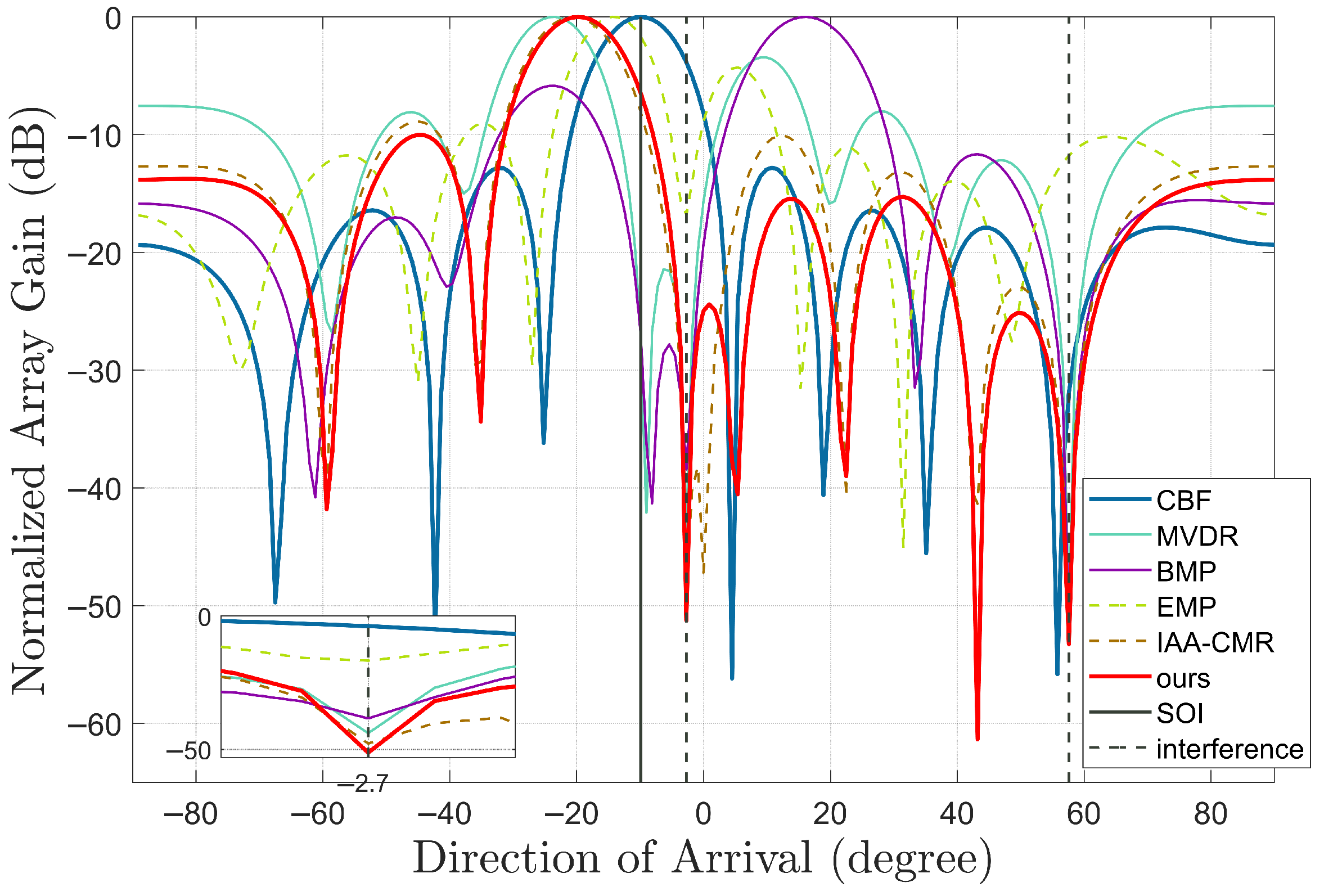
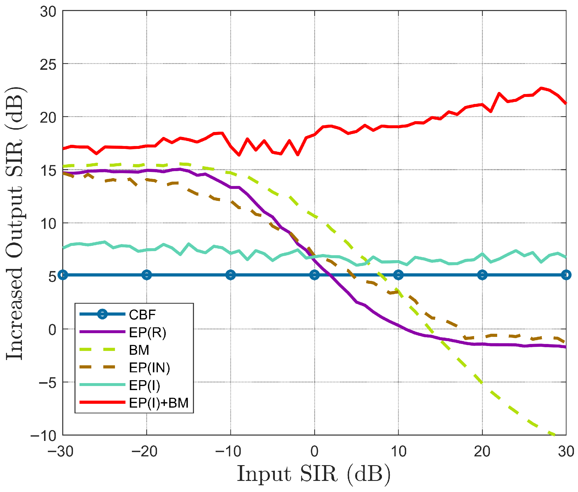
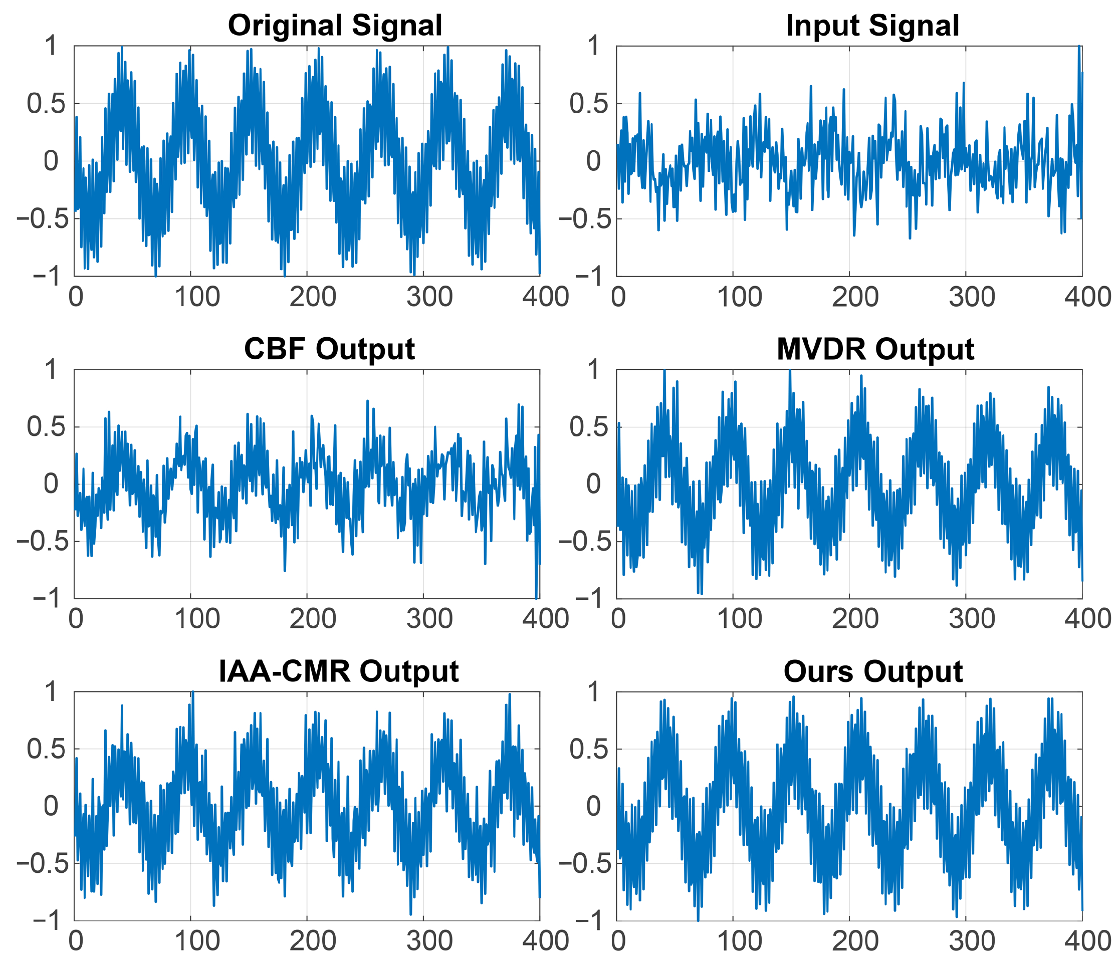
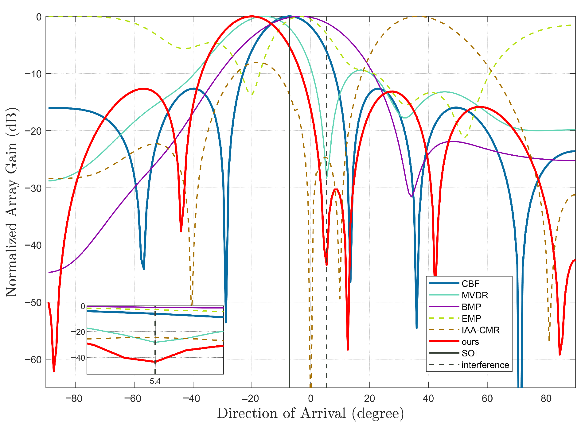
3.3. Interference Suppression Simulation
4. Results
5. Discussion
6. Conclusions
Author Contributions
Funding
Data Availability Statement
Conflicts of Interest
Abbreviations
| Symbol | Meaning | Symbol | Meaning |
| Expectation operator | The trace of the matrix | ||
| Hermite transpose of | max | Maximum value operator | |
| Hermitian positive definite square root of | Calculate the absolute value | ||
| L2 norm | diag | Construct a diagonal matrix using | |
| L1 norm | co | Coherence coefficient of a and b | |
| Abbreviation | Definition | Abbreviation | Definition |
| AUV | autonomous underwater vehicle | BMP | blocking matrix preprocessing |
| CBF | conventional beamforming | CMR | covariance matrix reconstruction |
| DOA | direction of arrival | EMP | eigen-projection matrix preprocessing |
| IAA | iterative adaptive approach | ICM | interference coherence matrix |
| INCM | interference and noise covariance matrix | MVDR | minimum variance distortionless response |
| MUSIC | multiple signal classification | SBL | sparse Bayesian learning |
| SOI | signal of interest | SIR | signal-to-interference ratio |
| SINR | signal-to-interference and noise ratio | SNR | signal-to-noise ratio |
| SPICE | sparse iterative covariance-based | ULA | uniform linear array |
References
- Ma, T.; Ding, S.; Li, Y.; Fan, J. A review of terrain aided navigation for underwater vehicles. Ocean Eng. 2023, 281, 114779. [Google Scholar] [CrossRef]
- Wang, F.-Q.-W.; Zhang, X.; Xing, X.-F.; Zhang, X.-J. The Research of Underwater Acoustic Detection System for Small AUV. In Proceedings of the 2015 Fifth International Conference on Instrumentation and Measurement, Computer, Communication and Control (IMCCC), Qinhuangdao, China, 18–20 September 2015; pp. 1828–1831. [Google Scholar]
- Maguer, A.; Dymond, R.; Grati, A.; Stoner, R.; Guerrini, P.; Troiano, L.; Alvarez, A. Ocean gliders payloads for persistent maritime surveillance and monitoring. In Proceedings of the 2013 OCEANS, San Diego, CA, USA, 23–27 September 2013. [Google Scholar]
- Zhang, Z.; Lin, M.; Li, D.; Wu, R.; Lin, R.; Yang, C. An AUV-Enabled Dockable Platform for Long-Term Dynamic and Static Monitoring of Marine Pastures. IEEE J. Ocean. Eng. 2025, 50, 276–293. [Google Scholar] [CrossRef]
- Zhang, M.; Tong, F.; Zhang, F.; Wei, B. CoralBuddy-1: A Micro-Sized Autonomous Underwater Vehicle for Offshore Coral Reef Monitoring. In Proceedings of the 17th International Conference on Underwater Networks & Systems, New York, NY, USA, 24–26 November 2023. [Google Scholar] [CrossRef]
- Hirotsu, R.; Ura, T.; Kojima, J.; Sugimatsu, H.; Bahl, R.; Yanagisawa, M. Classification of sperm whale clicks and triangulation for real-time localization with SBL arrays. In Proceedings of the OCEANS 2008, Quebec City, QC, Canada, 15–18 September 2008; p. 553. [Google Scholar]
- Wolek, A.; McMahon, J.; Dzikowicz, B.R.; Houston, B.H. Tracking Multiple Surface Vessels With an Autonomous Underwater Vehicle: Field Results. IEEE J. Ocean. Eng. 2022, 47, 32–45. [Google Scholar] [CrossRef]
- Chun, S.; Kawamura, C.; Ohkuma, K.; Maki, T. 3D Detection and Tracking of a Moving Object by an Autonomous Underwater Vehicle with a Multibeam Imaging Sonar: Toward Continuous Observation of Marine Life. IEEE Robot. Autom. Lett. 2024, 9, 3037–3044. [Google Scholar] [CrossRef]
- Glegg, S.A.L.; Olivieri, M.P.; Coulson, R.K.; Smith, S.M. A Passive Sonar System Based on an Autonomous Underwater Vehicle. IEEE J. Ocean. Eng. 2002, 26, 700–710. [Google Scholar] [CrossRef]
- Chi, C.; Pallayil, V.; Chitre, M. Design of an adaptive noise canceller for improving performance of an autonomous underwater vehicle-towed linear array. Ocean Eng. 2016, 202, 106886. [Google Scholar] [CrossRef]
- Xu, Y.; Kong, X.; Cai, Z. Cross-validation strategy for performance evaluation of machine learning algorithms in underwater acoustic target recognition. Ocean Eng. 2024, 299, 117236. [Google Scholar] [CrossRef]
- Li, J.; Tong, F.; Zhou, Y.; Yang, Y.; Hu, Z. Small Size Array Underwater Acoustic DOA Estimation Based on Direction-Dependent Transmission Response. IEEE Trans. Veh. Technol. 2022, 71, 12916–12927. [Google Scholar] [CrossRef]
- Aldeman, M.R. A hybrid spiral microphone array design for performance and portability. Appl. Acoust. 2020, 170, 107512. [Google Scholar] [CrossRef]
- Stoica, P.; Babu, P.; Li, J. SPICE: A Sparse Covariance-Based Estimation Method for Array Processing. IEEE Trans. Signal Process. 2011, 59, 629–638. [Google Scholar] [CrossRef]
- Stoica, P.; Babu, P. SPICE and LIKES: Two hyperparameter-free methods for sparse-parameter estimation. Signal Process. 2012, 92, 1580–1590. [Google Scholar] [CrossRef]
- Zhang, J.; Qu, H.; Li, R.; Chen, C.; Chen, W. Fast 2D Weighted Generalized Sparse Iterative Covariance-Based Estimation for Scanning Radar. IEEE Signal Process. Lett. 2025, 32, 2364–2368. [Google Scholar] [CrossRef]
- Dai, J.; Bao, X.; Xu, W.; Chang, C. Root Sparse Bayesian Learning for Off-Grid DOA Estimation. IEEE Signal Process. Lett. 2016, 24, 46–50. [Google Scholar] [CrossRef]
- Liang, Y.; Zheng, X.; Meng, W.; Li, J.; Chen, F. Noise Integral-Based Sparse Bayesian Learning for DOA Estimation Using Grid Pruning and Adaptation. Electron. Lett. 2025, 61, e70325. [Google Scholar] [CrossRef]
- Xing, C.; Wu, Y.; Xie, L.; Zhang, D. A sparse dictionary learning-based denoising method for underwater acoustic sensors. Appl. Acoust. 2021, 180, 108140. [Google Scholar] [CrossRef]
- Qian, J.; He, Z.; Jia, F.; Zhang, X. Mainlobe interference suppression in adaptive array. In Proceedings of the 2016 IEEE 13th International Conference on Signal Processing (ICSP), Chengdu, China, 6–10 November 2016; pp. 470–474. [Google Scholar] [CrossRef]
- Ma, X.; Jiang, S.; Zhang, S.; Zhang, R.; Sheng, W. Joint Wideband Beamforming Algorithm for Main Lobe Jamming Suppression in Distributed Array Radar. Remote Sens. 2024, 16, 2402. [Google Scholar] [CrossRef]
- Han, B.; Yang, X.; Lv, Q.; Li, W.; Zhang, Z.; Zhong, S. Mainlobe and sidelobe jamming suppression method based on distributed array radar with eigen-projection matrix processing and null constraints. IET Radar Sonar Navig. 2024, 18, 2212–2221. [Google Scholar] [CrossRef]
- Gu, Y.; Leshem, A. Robust Adaptive Beamforming Based on Interference Covariance Matrix Reconstruction and Steering Vector Estimation. IEEE Trans. Signal Process. 2012, 60, 3881–3885. [Google Scholar] [CrossRef]
- Wang, Y.; Bao, Q.; Chen, Z. Robust mainlobe interference suppression for coherent interference environment. EURASIP J. Adv. Signal Process. 2016, 2016, 135. [Google Scholar] [CrossRef]
- Wang, W.; Li, Y.; Shen, T.; Liu, F.; Zhao, D. An effective DOA estimation method for low SIR in small-size hydrophone array. Appl. Acoust. 2024, 217, 109848. [Google Scholar] [CrossRef]
- Ottersten, B.; Stoica, P.; Roy, R. Covariance Matching Estimation Techniques for Array Signal Processing Applications. Digit. Signal Process. 1998, 8, 185–210. [Google Scholar] [CrossRef]
- Stoica, P.; Zachariah, D.; Li, J. Weighted SPICE: A unifying approach for hyperparameter-free sparse estimation. Digit. Signal Process. 2014, 33, 1–12. [Google Scholar] [CrossRef]
- Li, R.F.; Wang, Y.L.; Wan, S.H. Robust adaptive beam forming under main lobe interference conditions. Syst. Eng. Electron. 2002, 24, 61–64. [Google Scholar]
- Zhou, J.; Bao, C.; Jia, M.; Xiong, W. A distortionless convolution beamformer design method based on the weighted minimum mean square error for joint dereverberation and denoising. Speech Commun. 2024, 158, 103054. [Google Scholar] [CrossRef]
- Pan, Y.; Zhang, L.; Xu, L.; Duan, F. DOA Estimation on One-Bit Quantization Observations through Noise-Boosted Multiple Signal Classification. Sensors 2024, 24, 4719. [Google Scholar] [CrossRef]


Disclaimer/Publisher’s Note: The statements, opinions and data contained in all publications are solely those of the individual author(s) and contributor(s) and not of MDPI and/or the editor(s). MDPI and/or the editor(s) disclaim responsibility for any injury to people or property resulting from any ideas, methods, instructions or products referred to in the content. |
© 2025 by the authors. Licensee MDPI, Basel, Switzerland. This article is an open access article distributed under the terms and conditions of the Creative Commons Attribution (CC BY) license (https://creativecommons.org/licenses/by/4.0/).
Share and Cite
Wang, W.; Li, Y.; Meng, L.; Shen, T.; Zhao, D. A Mainlobe Interference Suppression Method for Small Hydrophone Arrays. J. Mar. Sci. Eng. 2025, 13, 1348. https://doi.org/10.3390/jmse13071348
Wang W, Li Y, Meng L, Shen T, Zhao D. A Mainlobe Interference Suppression Method for Small Hydrophone Arrays. Journal of Marine Science and Engineering. 2025; 13(7):1348. https://doi.org/10.3390/jmse13071348
Chicago/Turabian StyleWang, Wenbo, Ye Li, Luwen Meng, Tongsheng Shen, and Dexin Zhao. 2025. "A Mainlobe Interference Suppression Method for Small Hydrophone Arrays" Journal of Marine Science and Engineering 13, no. 7: 1348. https://doi.org/10.3390/jmse13071348
APA StyleWang, W., Li, Y., Meng, L., Shen, T., & Zhao, D. (2025). A Mainlobe Interference Suppression Method for Small Hydrophone Arrays. Journal of Marine Science and Engineering, 13(7), 1348. https://doi.org/10.3390/jmse13071348