A Revised Model of the Ocean’s Meridional Overturning Circulation

Abstract

This work explores the density-driven overturning circulation of the ocean using a process-oriented three-dimensional hydrodynamic model with a free sea surface. As expected, dense-water formation in polar regions creates a deep western boundary current (DWBC) spreading southward along the continental slope. Near the equator, the DWBC releases its water eastward into the ambient ocean to form a large upwelling zone. This upwelling is coupled with a slow westward surface recirculation feeding into a swift surface return flow along the western boundary that closes the mass budget. This recirculation pattern, which is fundamentally different to the Stommel–Arons model, is a consequence of geostrophic adjustment to anomalies of the surface pressure field that form under the influence of both coastal and equatorial Kelvin waves and Rossby waves. Based on the findings, the author presents a revised model of the ocean’s meridional overturning circulation to supersede earlier, incorrect suggestions.

1. Introduction

The general circulation of the ocean comprises the wind-driven circulation (dominating the upper 1–2 km of the water column) and the density-driven deep circulation, which is driven by the regional formation and spreading of anomalously dense seawater. Their coupling plays an important role in the climate system, particularly in the North Atlantic where the formation, sinking and spreading of North Atlantic Deep Water induces an enhanced northward heat transport that reaches as far as into the subsurface layers of the Arctic Ocean [1].

This work explores the structure and dynamics of the ocean’s deep circulation that follows from the sinking of dense water at high latitudes. This topic has been scientifically debated for more than 65 years. The starting point of this debate is the classical Stommel–Arons model [2,3] that was motivated by laboratory experiments [4]. The model is still widely used in classroom teaching and frequently cited in scientific research [5,6]. The key element of the Stommel–Arons model is the law of mass conservation. This law implies that the vertical volume flux due to sinking of dense water at high latitudes must be balanced by the same volume flux due to upwelling elsewhere. The key assumption underlying the Stommel–Arons model is that this upwelling is spatially uniform throughout the North Atlantic, which due to vortex stretching implies a poleward geostrophic flow. Again, due to mass conservation, this poleward flow then needs to be counterbalanced by an equatorward deep western boundary current (DWBC), which feeds mass to both the poleward recirculation and the upwelling across the domain. See [7] for a thorough review of the Stommel–Arons Model.

Munk [8] took the known sinking rate for the world ocean (~30 Sv; 1 Sv = 10⁶ m³ s⁻¹) and argued that if it returns uniformly to the surface, the one-dimensional vertical heat and salt balance would require a vertical mixing coefficient of the order of 10⁻⁴ m²/s. Given that this mixing rate is ten times greater than widely observed (e.g., [9,10,11]), the insufficient amount of vertical mixing is at odds with the Stommel–Arons model (e.g., [6]). According to [12], two main threads have been followed to resolve this apparent conundrum. The first focusses on finding the missing mixing, which has led to substantial observational efforts (e.g., [5,13]). The second has identified the Southern Ocean as a conduit for the overturning flow (e.g., [14]).

Contrary to expectations, early numerical simulations of the North Atlantic by Holland [15] generated a dominant upwelling pathway within a few grid points from the deep western boundary current and downwelling (instead of upwelling) in the remainder of the domain. Veronis [16] suggested that this feature was the result of physically unrealistic mixing near the western boundary, called the “Veronis effect”. McDougall and Church [17] used a similar reasoning in their interpretation of modelling results by Cox and Bryan [18]. For many years, unusual upwelling near the western boundary in Ocean General Circulation Models (OGCMs) simulations has been regarded as biased and undesired, and efforts were made to eliminate this effect. For instance, McDougall & Church [17], Redi [19] and Cox [20] developed parameterizations of isopycnal/diapycnal mixing that have been used since in many OGCMs. See [21,22] for references. Gent & McWilliams [23] introduced a new parameterization for eddy-induced transport which avoided the use of a horizontal diffusion term and reduced the biases attributed to the Veronis effect [24,25,26]. While these parameterizations mimic density fluxes associated with mesoscale eddies on scales not resolved in OGCMs, how much they lead to a bias of other dynamical features has not been addressed.

Earlier ocean circulation models did not account for a free sea surface responding to horizontal flow divergence in the water column underneath. Similarly, there are ample investigations of the deep circulation that used layer models that excluded a free sea surface [27,28,29,30,31,32,33]. These models were either formulated as 1½-layer reduced-gravity models, or as 2-layer reduced-gravity models driven by a diapycnal mass flux across the density interface. Neither of these model applications accounted for the effect that the density-driven flows have on surface pressure field and the surface currents resulting from them.

Could it be that the current understanding of the deep circulation has been misguided by a generation of studies based on numerical models that missed an important part of the dynamics arising from barotropic pressure gradients that are directly formed by the DWBC? This paper revisits the dynamics of the DWBC using a three-dimensional hydrodynamic model with a free sea surface. In contrast to most previous studies, the findings indicate that the DWBC creates a dominant overturning circulation along the western boundary with an upwelling zone in the western equatorial Atlantic.

2. Methodology

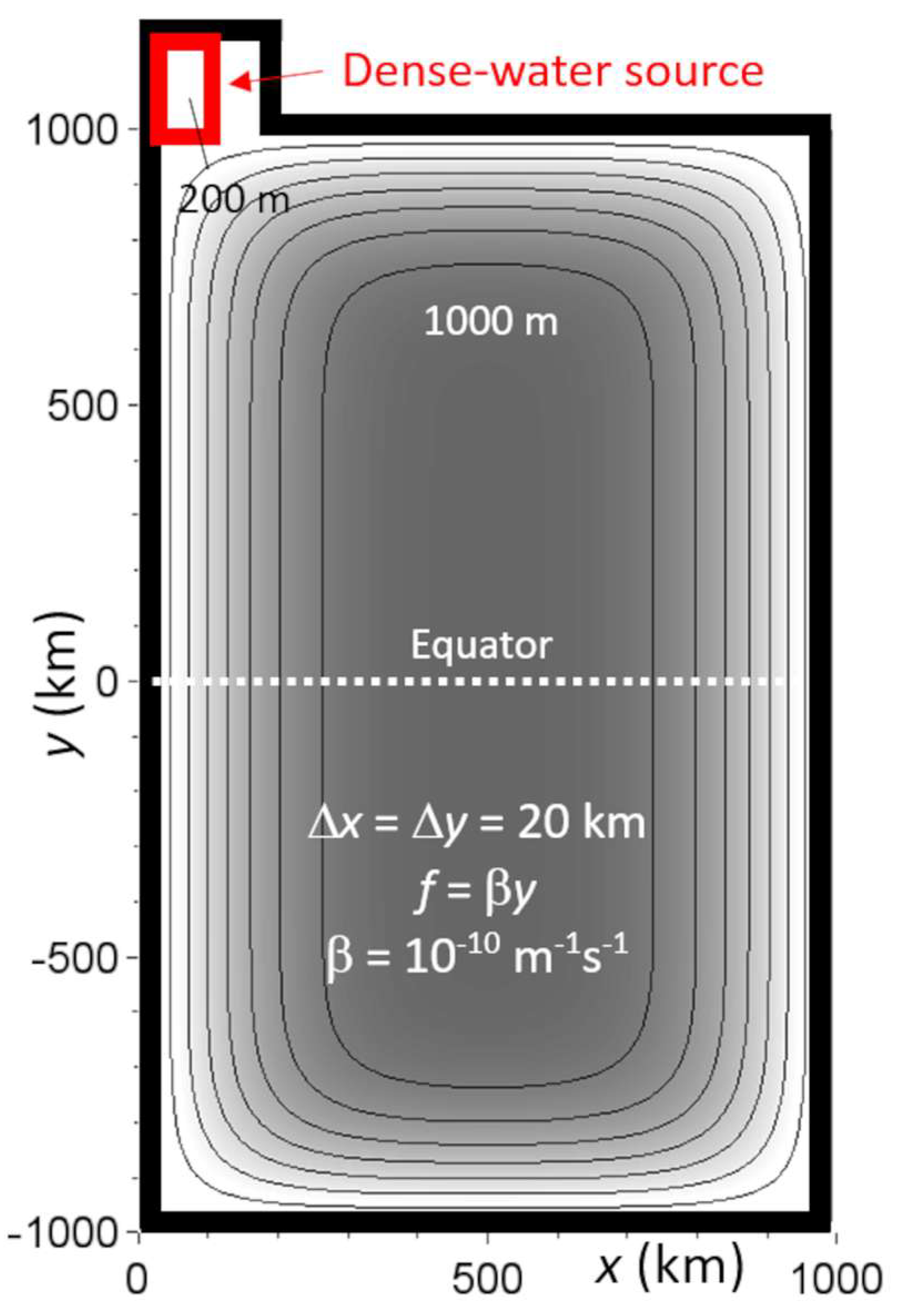
2.1. Model Description

This study employs the three-dimensional COHERENS hydrodynamic model [34]. In Cartesian coordinates, the physical conservation equations governing the model can be written as [35]:

$$\partial u/\partial t+\mathrm{A}\mathrm{d}\mathrm{v}\left(u\right)-fv=-1/{\rho }_o\partial \left(p+q\right)/\partial x+\mathrm{D}\mathrm{i}\mathrm{f}\mathrm{f}\left(u\right)$$

(1)

$$\partial v/\partial t+\mathrm{A}\mathrm{d}\mathrm{v}\left(v\right)+fu=-1/{\rho }_o\partial \left(p+q\right)/\partial y+\mathrm{D}\mathrm{i}\mathrm{f}\mathrm{f}\left(v\right)$$

(2)

$$\partial w/\partial t+\mathrm{A}\mathrm{d}\mathrm{v}\left(w\right)=-1/{\rho }_o\partial q/\partial z+\mathrm{D}\mathrm{i}\mathrm{f}\mathrm{f}\left(w\right)$$

(3)

$$\partial \rho /\partial t+\mathrm{A}\mathrm{d}\mathrm{v}\left(\rho \right)=\mathrm{D}\mathrm{i}\mathrm{f}\mathrm{f}\left(\rho \right)$$

(4)

$$\partial u/\partial x+\partial v/\partial y+\partial w/\partial z=0$$

(5)

$$\partial p/\partial z=-\left(\rho -{\rho }_o\right)g$$

(6)

$$\partial q_s/\partial t=-{\rho }_{o}g\left[\partial \left(h〈u〉\right)/\partial x+\partial \left(h〈v〉\right)/\partial y\right]$$

(7)

where (u, v, w) is the velocity vector; dynamic pressure is expressed as P = p + q, with p representing the hydrostatic pressure field related to a flat surface, calculated from (6), and q representing the nonhydrostatic pressure field; (x, y, z) are the spatial coordinates; ρ is seawater density with a reference value of ρ_o = 1026 kg m⁻³; f is the Coriolis parameter; Adv(.) and Diff(.) are three-dimensional advection and diffusion operators; g = 9.81 m s⁻² is vertical acceleration due to gravity; h is total water depth; and q_s = ρ_ogη (η is sea-surface elevation) refers to the surface value of q. Equations (1)–(7) are the full traditional Navier–Stokes equations for an incompressible fluid under the Boussinesq approximation. The momentum equations, (1)–(3), are connected via the continuity equation (5). Anomalies of the density field are predicted from (4), directly influences the hydrostatic pressure according to (6). Eventually, (7) expresses how horizontal currents influence the free surface and hence the surface dynamic pressure field. The COHERENS model converts these equations into a terrain-following σ coordinate system. This model is based on the same physical laws and coordinate transformation and similar numerical algorithms that govern other sigma coordinate models such as POM [36] or ROMS [37].

The Smagorinsky closure scheme [38] is used to parameterize horizontal turbulence. The k-ε turbulence closure using standard parameter settings (see [34]) is applied to parameterize vertical turbulence. Surface stresses are set to zero; that is, wind forcing is not considered here. This model configuration directly predicts changes in the seawater density field from an advection–diffusion equation in which eddy diffusivities are identical to eddy viscosities. Bottom friction is parameterized using a quadratic approach. The bottom friction coefficient, C_D, is expressed by a roughness length, δ, via the relationship (see [34]):

C_D = [ln(z*/δ)/κ]⁻²

(8)

where z* is the distance of the bottom-nearest horizontal velocity grid point to the seafloor and κ = 0.4 is the von Kármán constant. A uniform roughness length of δ = 2 mm is used in all simulations. Variations of turbulence parameters and bottom friction had no significant influence on the results.

2.2. Experimental Design

The model domain (Figure 1) mimics the main bathymetric and geographic aspects of the Atlantic Ocean including a dense-water formation in the north, a continental margin and an equator. The model domain is cast on the β-plane, i.e., f = βy, where y = 0 defines the equator, using an artificially inflated value of β = 10⁻¹⁰ m⁻¹ s⁻¹. This yields a value of |f| = 1 × 10⁻⁴ s⁻¹ at y = ± 1000 km, corresponding to mid-latitudes in the real world. The inflation of the β parameter allows for the use of a relatively small model domain while retaining the full range of the Coriolis parameter. The model domain is a largely rectangular ocean basin that is 1000 km wide and 2200 km long, resolved by horizontal grid spacings of Δx = Δy = 20 km. A large bay, 200 m deep, located in the northwestern corner of the model domain, serves as the source of dense water driving the simulated deep circulation. For simplicity, the model ocean is fully enclosed by coasts, which ignores influences of the Southern Ocean in the South Atlantic. The bathymetry is spatially variable, ranging from 200 m on the continental shelf to 1000 m in the deepest parts of the domain. The water column is resolved by 20 sigma layers in the vertical. The continental slope has an inclination of 0.0035 (0.2°).

The water column is initialized with a horizontally uniform vertical density profile. Initially, seawater density is uniform with a value of 1024.2 kg m⁻³ in a 100 m deep surface mixed layer, then linearly increases to 1025.0 kg m⁻³ at a depth of 200 m at a stability frequency of N = 0.01 s⁻¹, from where it continues to linearly increase to 1026.6 kg m⁻³ at a depth of 1000 m at a stability frequency of N = 0.004 s⁻¹.

The model is forced by gradually increasing seawater in the region of dense-water formation (see Figure 1) throughout the water column according to:

$$\partial \rho /\partial t=Q$$

(9)

where the source term is set to $Q$ = 0.8/(30 × 24 × 3600) kg m⁻³ s⁻¹; that is, density increases by 0.8 kg m⁻³ on a timescale of 30 days. Maximum density is limited to 1025.8 kg m⁻³. With this target density, the newly formed dense water can be expected to spread along an equilibrium horizon at a depth of ~600 m. Otherwise, there are no surface density fluxes across the model domain. Variations of Q yielded similar results.

Three different passive Eulerian tracer fields, C_lat, C_long and C_source, are used to visualize horizontal advection patterns associated with the simulated overturning circulation. Initially, C_lat increases linearly along the y axis according to (Figure 2a):

$$C_{\mathrm{lat}}(x,y,z)=\mathrm{m}\mathrm{i}\mathrm{n}\left[(y-1000)/\mathrm{2000,1}\right]$$

(10)

where y is expressed in km. Anomalies in C_lat highlight meridional advection effects. Similarly, C_long increases initially linearly along the x axis according to (Figure 2b):

$$C_{\mathrm{long}}(x,y,z)=x/1000$$

(11)

Anomalies in C_long highlight zonal advection effects. Another Eulerian concentration field, C_source, is used to trace the newly formed dense water. Starting with zero values throughout the computational domain, C_source is kept at a value of unity in the region of dense-water formation (see Figure 1) throughout the simulation. The evolution of the tracer fields is predicted from a prognostic advection–diffusion equation that is identical to that used for the density field. The total simulation time of experiments is 500 days.

In addition, Lagrangian particles are initially placed in every grid cell across the model domain at a depth horizon of 200 m. Vertical displacements due to upwelling or downwelling are then calculated from the kinematic equation:

$$d{z}^{\ast }/dt=\mathrm{w}$$

(12)

where z^* is the vertical location of a particle, and w is the predicted time-variable vertical velocity component interpolated onto this location. Horizontal displacements and turbulence effects are ignored. The resultant net displacements are then converted to a horizontal map of average vertical velocities. Using a numerical time step of Δt = 100 s, which is constrained by the CFL stability criteria for surface gravity waves, the total simulation time of the numerical experiment is 3 years. Generative artificial intelligence (GenAI) was not used for any aspect of this research including text, data and graphics generation, study design, analysis and interpretation.

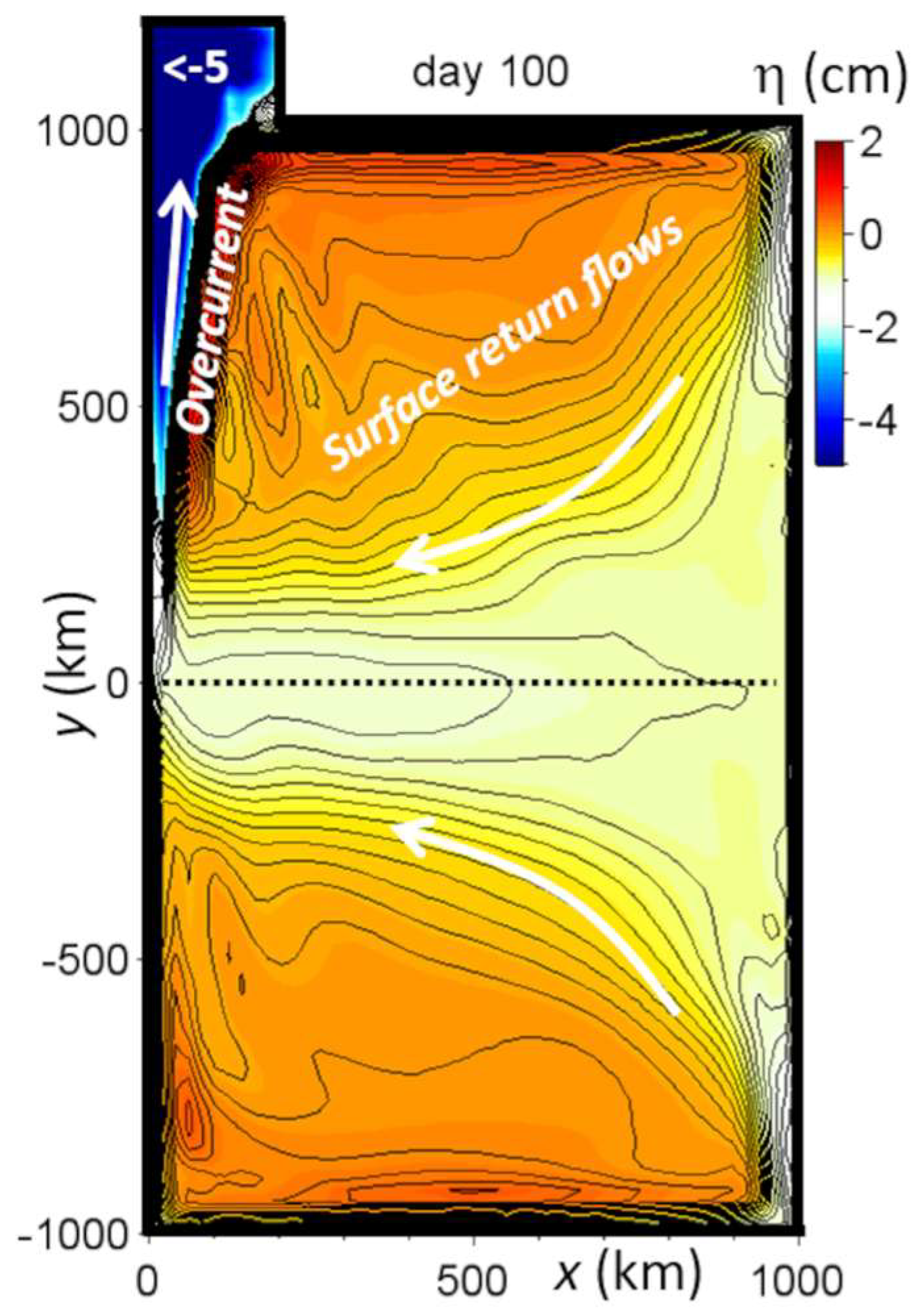
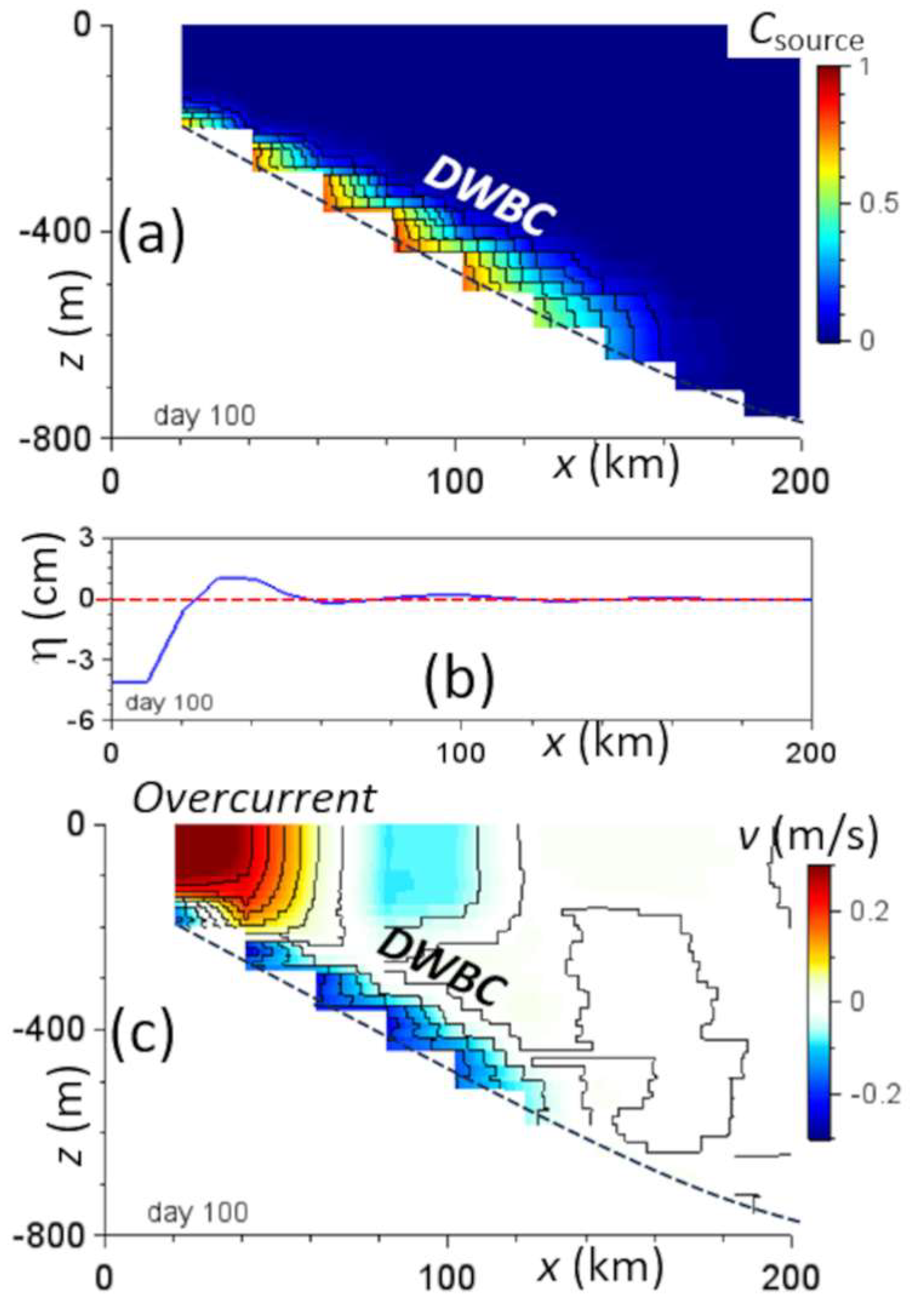
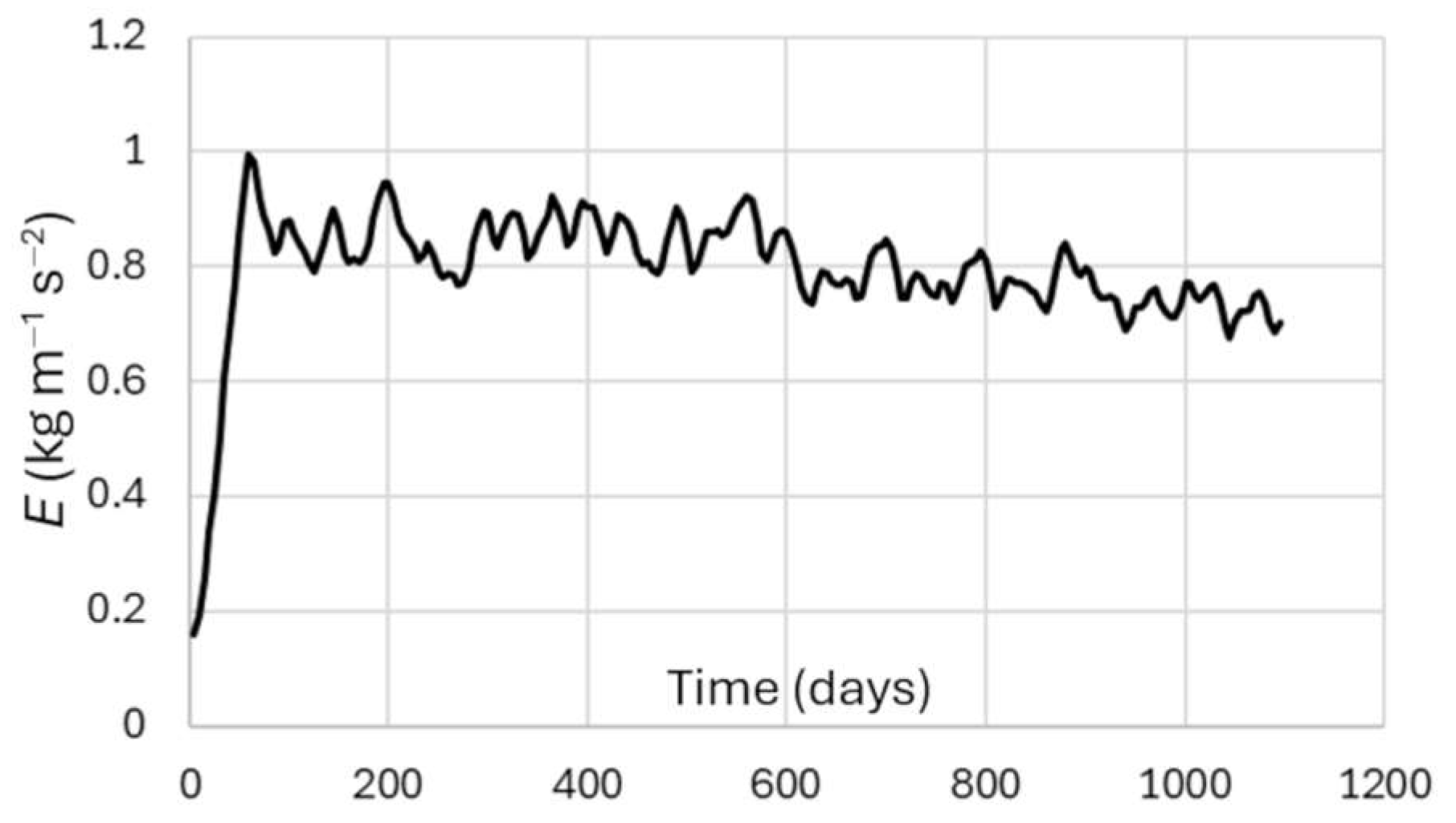
3. Results and Discussion

As expected, dense-water formation in the northwestern corner of the model domain creates a DWBC spreading southward along the continental slope (Figure 3a). After 50 days of simulation, the DBWC almost reaches the equator. On the other hand, a northward surface boundary current appears near the western boundary (Figure 3b), obviously to conserve mass in the dense-water formation region.

Horizontal gradients of sea-surface elevation η are the principal driver of the quasi-geostrophic surface circulation. Dense-water formation initiates here a southward dense-water overflow, akin to the Denmark Strait Overflow [32]. This overflow leads to a mass deficit in the formation region, such that the sea level drops. In return, the resultant northward barotropic pressure gradient induces a surface return flow that soon (within a matter a days) develops into a geostrophically driven poleward surface boundary current, henceforth called “overcurrent“ (Figure 4). The equilibrium is characterized by η ≈ ~17.5 cm in the dense-water formation region.

Under the action of a coastal Kelvin wave, the negative sea-level anomaly gradually spreads southward along the west coast. The negative sea-level anomaly then continues to spread eastward along the equator as the signature of equatorial Kelvin waves, before turning poleward along the eastern boundaries in the form of coastal Kelvin waves. On the other hand, Rossby waves emanate from the eastern boundary. On a timescale > 50 days, the surface pressure field created by these waves becomes a stationary feature. Prominent features of this surface pressure field are (i) strong onshore pressure gradients all along the western boundary of the model’s North Atlantic, and (ii) weak but persistent equatorward pressure gradients in the open ocean.

The resultant quasi-geostrophic surface circulation pattern is fundamentally different from the Stommel–Arons model that postulated a northward surface flow throughout the entire domain.

Vertical transects across the center of the model’s North Atlantic at y = 500 km (see Figure 1) reveal the vertical structure of the simulated boundary currents (Figure 5). Here, we can see that the simulated DWBC is a bottom-arrested feature that spreads southward along the continental slope in a depth range of 300–700 m (Figure 5a). Note that this spreading is influenced by bottom-parallel “horizontal” turbulent diffusion in the σ-coordinate model. The plume attains a thickness of ~100 m and a southward speed of ~0.2 m/s (Figure 5c). Geostrophic adjustment theory for a two-layer fluid gives a speed of the reduced gravity plume of (e.g., [39]):

v = (g’ h)^1/2

(13)

where g’ = Δρ/ρ_o g is reduced gravity, and h is the thickness of the reduced-gravity plume. For Δρ = 0.1 kg m⁻³, ρ_o = 1025 kg m⁻³ and h = 100 m, we yield v = 0.31 m s⁻¹, which is close to the simulated value. A negative coastal sea-level anomaly of −4 cm is established near the coast creating an onshore barotropic pressure gradient within 40 km from the coast (Figure 5b). This onshore pressure gradient creates the western overcurrent with a speed of ~0.3 m/s (see Figure 5c). It is obvious that this overcurrent plays a central part in the simulated meridional overturning circulation. Other surface flows in the open ocean attain small geostrophic speeds ~5 mm s⁻¹, which correspond to sea-level gradients of 1 cm on a length scale of 400 km and a Coriolis parameter of f = 0.5 × 10⁻⁴ s⁻¹.

Note that the formation of surface flows (i.e., the overcurrent simulated here) is a characteristic feature inherent with the geostrophic–gravitational adjustment of a two-layer fluid. This fundamental feature, arising from vortex stretching/squeezing of the fluid layers, has been demonstrated both analytically [40] and in numerical/laboratory experiments [41]. However, the situation discussed here differs from the stand-alone adjustment process as it involves coastal Kelvin waves as an active ingredient.

In terms of kinetic energy density, a dynamic equilibrium is established within 50 days of simulation (Figure 6). This timescale is like that in previous simulations of the dynamics of boundary currents (e.g., [42]). The kinetic energy density remains close to the value of 0.8 kg m⁻¹ s⁻² throughout the simulation, with some short-term variability of periods ~10–20 days.

Near the formation region, the dense-water overflow has a volume transport of Q ~ 1 Sv throughout the simulation (Figure 7). During the initial 100 days, the DWBC extends to the equator with a fourfold increase of the volume transport along its pathway (Figure 7a). The volume transport decreases south of the equator. During 400 days of simulation, Q increases from the formation region to ~8 Sv at y ≈ 350 km (Figure 7b). From this maximum, it gradually decreases in a linear fashion to zero at the southern boundary. Maximum values of Q ~6 Sv are sustained for the remainder of the simulation over a relatively large latitude range of y ≈ 250–750 km (Figure 7c). The distributions between 500 and 800 days of simulation indicate establishment of a dynamical equilibrium.

It should be highlighted that the western overcurrent attains identical volume-transport distributions. Hence, the simulated meridional overturning circulation primarily takes place close to the western boundary. Note that volume transports associated with the simulated overturning circulation are fivefold smaller than in the real situation, which can be attributed to the relatively weaker dense-water overflows. For instance, the volume transport of the Denmark Strait overflow alone is 3.2 Sv [43], which exceeds that simulated here threefold.

Along its path, the simulated DWBC boundary entrains ambient water such that the value of C_source decreases slightly from unity in the formation region to 0.7 near the equator (Figure 8a). The DWBC continues its southward flow across the equator over ~600 km after 500 days of simulation. As anticipated, the DWBC spreads along its equilibrium density horizon around 600 m (Figure 8b). Near the equator, a fraction of seawater carried by the boundary current is injected eastward into the ambient water column where it creates a broad upwelling zone. The predicted pathway of the DWBC including eastward flows near the equator agrees well with observational evidence [44]. The upwelling zone in the model’s western equatorial Atlantic is characterized by upwelling speeds of w = 50–100 m/year (at a depth of 200 m), whereas lower upwelling speeds of w = 20–30 m/year are predicted in large regions across the open ocean (Figure 8c). Notable is the formation of a downwelling region on the eastern side of the equator with downwelling speeds of ~−50 m/year.

The distortion of the Eulerian tracer field C_lat shows the northward advection of the western overcurrent after 500 days of simulation (Figure 9a) which remains a robust circulation feature during the entire circulation. The tracer distribution also indicates eastward flows along the northern and southern boundaries. On the other hand, the advective distortion of the Eulerian tracer field C_long reveals the westward return flow near the equator, noting that the curvy pattern of the distribution is the result of westward-propagating planetary Rossby waves.

4. Final Discussion

Application of a free-surface, three-dimensional hydrodynamic model predicts a meridional overturning circulation that is fundamentally different from the Stommel–Arons model. Instead of a poleward recirculation in the open ocean, here the recirculation takes place in a swift, narrow coastal surface return flow, called “western overcurrent”, and a slow westward drift accompanied by an extensive upwelling zone in the western equatorial Atlantic (Figure 10). The results demonstrate that this overcurrent is a direct consequence of the effect that the formation and spreading of dense water has on the dynamical shape of the sea surface (driving geostrophic surface currents). Early models of the meridional overturning circulation based on the Stommel–Arons model [2,3,4] do not account for this fundamental coupling mechanism. Despite its limitations and flaws, the Stommel–Arons model has made significant contributions to the understanding of the ocean’s deep circulation.

The predicted pathway of the DWBC is consistent with observations [42]. Interestingly, the current model simulation predicts upwelling across most of the open ocean, which is consistent with vertical mixing theories [8], but this weak upwelling is not induced here by poleward flows.

In this study, inflation of the value of the beta parameter influenced the kinematics of planetary waves, including mixed Rossby-gravity waves trapped along the equator. Further studies are required to study the dynamics of the western overcurrent in full-scale spherical coordinates and in configurations that include wind forcing and the Southern Ocean.

Many, if not all, modern OGCMs include the option of a free sea surface and therefore are able to simulate (but not necessarily resolve) the western overcurrent. Therefore, it is worthwhile to critically analyze the effects that parameterizations developed to eliminate the Veronis effect in OGCMs have on the overturning circulation. In the real world, it can be expected that the wind-driven surface circulation overshadows the western overcurrent in many regions. Future studies should focus on regions where this overflow can possibly be directly observed and mechanisms that can influence the dynamics of the overcurrent. Findings presented in this paper have significant implications for the understanding of both the ocean’s meridional overturning and vertical mixing in the oceans.

References

1. Tomczak, M.; Godfrey, J.S. Regional Oceanography: An Introduction, 2nd ed.; Daya Publishing House: Delhi, India, 2003; 390p. [Google Scholar]
2. Stommel, H.; Arons, A.B. On the abyssal circulation of the world ocean: I. Stationary planetary flow patterns on a sphere. Deep-Sea Res. 1960, 6, 140–154. [Google Scholar] [CrossRef]
3. Stommel, H.; Arons, A.B. On the abyssal circulation of the world ocean: II. An idealized model of the circulation pattern and amplitude in oceanic basins. Deep-Sea Res. 1960, 6, 217–233. [Google Scholar] [CrossRef]
4. Stommel, H.; Arons, A.B.; Faller, A.J. Some examples of stationary flow patterns in bounded basins. Tellus 1958, 10, 179–187. [Google Scholar] [CrossRef]
5. Ferrari, R.; Mashayek, A.; McDougall, T.J.; Nikurashin, M.; Campin, J. Turning ocean mixing upside down. J. Phys. Oceanogr. 2016, 46, 2239–2261. [Google Scholar] [CrossRef]
6. Wunsch, C. A simplified ocean physics? Revisiting Abyssal Recipes. J. Phys. Oceanogr. 2023, 53, 1387–1400. [Google Scholar] [CrossRef]
7. Pedlosky, J. Ocean Circulation Theory; Springer: New York, NY, USA, 2004; 453p. [Google Scholar]
8. Munk, W.H. Abyssal recipes. Deep-Sea Res. Oceanogr. Abstr. 1966, 13, 707–730. [Google Scholar] [CrossRef]
9. Waterhouse, A.F.; MacKinnon, J.A.; Nash, J.D.; Alford, M.H.; Kunze, E.; Simmons, H.L.; Polzin, K.L.; Laurent, L.C.S.; Sun, O.M.; Pinkel, R.; et al. Global patterns of diapycnal mixing from measurements of the turbulent dissipation rate. J. Phys. Oceanogr. 2014, 44, 1854–1872. [Google Scholar] [CrossRef]
10. Gregg, M.C. Ocean Mixing; Cambridge University Press: Cambridge, UK, 2021; 378p. [Google Scholar]
11. Moum, J.N. Variations in ocean mixing from seconds to years. Ann. Rev. Mar. Sci. 2021, 13, 201–226. [Google Scholar] [CrossRef]
12. Burchard, H.; Alford, M.; Chouksey, M.; Dematteis, G.; Eden, C.; Giddy, I.; Klingbeil, K.; Boyer, A.L.; Olbers, D.; Pietrzak, J.; et al. Linking Ocean Mixing and Overturning Circulation. Bull. Am. Meteorol. Soc. 2024, 105, E1265–E1274. [Google Scholar] [CrossRef]
13. Polzin, K.L. An abyssal recipe. Ocean Model. 2009, 30, 298–309. [Google Scholar] [CrossRef]
14. Cessi, P. The global overturning circulation. Annu. Rev. Mar. Sci. 2019, 11, 249–270. [Google Scholar] [CrossRef] [PubMed]
15. Holland, W.R. Ocean tracer distributions. I. A preliminary numerical experiment. Tellus 1971, 23, 371–392. [Google Scholar] [CrossRef]
16. Veronis, G. The role of models in tracer studies. In Numerical Models of Ocean Circulation 1975, Proceedings of a symposium held at Durham, New Hampshire, Durham, NH, USA, 17–20 October 1972; National Academy of Sciences: Washington, DC, USA; pp. 133–146.
17. McDougall, T.; Church, J. Pitfalls with the numerical representation of isopycnal and diapycnal mixing. J. Phys. Oceanogr. 1985, 17, 1950–1964. [Google Scholar] [CrossRef]
18. Cox, M.; Bryan, K. A numerical model of the ventilated thermocline. J. Phys. Oceanogr. 1984, 14, 674–687. [Google Scholar] [CrossRef]
19. Redi, M.H. Oceanic isopycnal mixing by coordinate rotation. J. Phys. Oceanogr. 1982, 12, 1154–1158. [Google Scholar] [CrossRef]
20. Cox, M.D. An eddy-resolving numerical model of the ventilated thermocline: Time dependence. J. Phys. Oceanogr. 1987, 17, 1044–1056. [Google Scholar] [CrossRef]
21. Gough, W.A.; Lin, C.A. Isopycnal mixing and the Veronis effect in an ocean general circulation model. J. Mar. Res. 1995, 53, 189–199. [Google Scholar] [CrossRef]
22. Lazar, A.; Madec, G.; Delecluse, P. The deep interior downwelling, the Veronis effect, and mesoscale tracer transport parameterizations in an OGCM. J. Phys. Oceanogr. 1999, 29, 2945–2961. [Google Scholar] [CrossRef]
23. Gent, P.R.; McWilliams, J.C. Isopycnal mixing in ocean circulation models. J. Phys. Oceanogr. 1990, 20, 150–155. [Google Scholar] [CrossRef]
24. Böning, C.W.; Holland, W.R.; Bryan, F.O.; Danabasoglu, G.; McWilliams, J.C. An overlooked problem in model simulations of the thermohaline circulation and heat transport in the Atlantic Ocean. J. Clim. 1995, 8, 515–523. [Google Scholar] [CrossRef]
25. Danabasoglu, G.; McWilliams, J.C. Sensitivity of the global ocean circulation to parameterizations of mesoscale tracer transports. J. Clim. 1995, 8, 2967–2987. [Google Scholar] [CrossRef]
26. Weaver, A.J.; Eby, M. On the numerical implementation of advection schemes for use in conjunction with various mixing parameterizations in the GFDL ocean model. J. Phys. Oceanogr. 1997, 27, 369–377. [Google Scholar] [CrossRef]
27. Kawase, M. Establishment of deep ocean circulation driven by deep-water production. J. Phys. Oceanogr. 1987, 17, 2294–2317. [Google Scholar] [CrossRef]
28. Hautala, S.L.; Riser, S.T. A simple model of abyssal circulation, including effects of wind, buoyancy, and topography. J. Phys. Oceanogr. 1989, 19, 596–611. [Google Scholar] [CrossRef]
29. Straub, D.N.; Rhines, P.B. Effects of large-scale topography on abyssal circulation. J. Mar. Res. 1990, 48, 223–253. [Google Scholar] [CrossRef]
30. Straub, D.N.; Killworth, P.D.; Kawase, M. A simple model of mass-driven abyssal circulation over a general bottom topography. J. Phys. Oceanogr. 1993, 23, 1454–1469. [Google Scholar] [CrossRef]
31. Karcher, M.; Lippert, A. Spin-up and breakdown of source-driven deep North Atlantic flow over realistic bottom topography. J. Geophys. Res. 1994, 99, 12357–12373. [Google Scholar] [CrossRef]
32. Spall, M.A. Large-Scale Circulations Forced by Localized Mixing over a Sloping Bottom. J. Phys. Oceanogr. 2001, 31, 2369–2384. [Google Scholar] [CrossRef]
33. Andersson, H.C.; Veronis, G. Thermohaline circulation in a two-layer model with sloping boundaries and a mid-ocean ridge. Deep. Sea Res. Part I Oceanogr. Res. Pap. 2004, 51, 93–106. [Google Scholar] [CrossRef]
34. Luyten, P.J.; Jones, J.E.; Proctor, R.; Tabor, A.; Tett, P.; Wild-Allen, K. COHERENS-A Coupled Hydrodynamical-Ecological Model for Regional and Shelf Seas: User Documentation; MUMM Report; Management Unit of the North Sea: Brussels, Belgium, 1999; 914p, Available online: https://uol.de/f/5/inst/icbm/ag/physoz/download/from_emil/COHERENS/print/userguide.pdf (accessed on 10 June 2025).
35. Kämpf, J. Advanced Ocean Modelling; Springer: Berlin/Heidelberg, Germany, 2010; pp. 125–127. [Google Scholar]
36. Blumberg, A.F.; Mellor, G.L. A description of a three-dimensional coastal ocean circulation model. In Three-Dimensional Coastal Ocean Models Coastal and Estuarine Sciences; Heaps, N.S., Ed.; American Geophysical Union: Washington, DC, USA, 2013; Volume 4, pp. 1–16. [Google Scholar] [CrossRef]
37. Shchepetkin, A.F.; McWilliams, J.C. The regional oceanic modeling system (ROMS): A split-explicit, free-surface, topography-following-coordinate oceanic model. Ocean Model. 2005, 9, 347–404. [Google Scholar] [CrossRef]
38. Smagorinsky, J. General circulation experiments with the primitive equations. I: The basic experiment. Mon. Weath. Rev. 1963, 91, 99–164. [Google Scholar] [CrossRef]
39. Jungclaus, J.H.; Backhaus, J.O. Application of a transient reduced gravity plume model to the Denmark Strait Overflow. J. Geophys. Res. 1994, 99, 12375–12396. [Google Scholar] [CrossRef]
40. Cushman-Roisin, B.; Beckers, J.-M. Introduction to Geophysical Fluid Dynamics, 2nd ed.; Academic Press: Cambridge, MA, USA, 2011; 875p. [Google Scholar]
41. Kämpf, J. Cascading-driven upwelling in submarine canyons at high latitudes. J. Geophys. Res. 2005, 110, C02007. [Google Scholar] [CrossRef]
42. Weaver, A.J.; Middleton, J.H. An analytic model for the Leeuwin Current of West Australia. Cont. Shelf Res. 1990, 10, 105–122. [Google Scholar] [CrossRef]
43. Jochumsen, K.; Moritz, M.; Nunes, N.; Quadfasel, D.; Larsen, K.M.H.; Hansen, B.; Valdimarsson, H.; Jonsson, S. Revised transport estimates of the Denmark Strait overflow. J. Geophys. Res. Oceans 2017, 122, 3434–3450. [Google Scholar] [CrossRef]
44. Richardson, P.L.; Fratantoni, D.M. Float trajectories in the deep western boundary current and deep equatorial jets of the tropical Atlantic. Deep-Sea Res. Part II Top. Stud. Oceanogr. 1999, 46, 305–333. [Google Scholar] [CrossRef]
Figure 1. Model configuration. Bathymetry (gray shading and contours; CI = 100 m). The line along y = 0 defines the equator. The region of dense-water formation is in the northwestern corner of the model domain (red rectangle) spanning 5 grid points in the x-direction and 10 grid points in the y-direction.
Jmse 13 01244 g001
Figure 2. Initial horizontal distributions of the passive Eulerian tracers (a) Clat and (b) Clong (color shading). See the text for their definitions. Full lines are bathymetric contours (CI = 100 m). The dotted line highlights the equator.
Jmse 13 01244 g002
Figure 3. (a) Surface and (b) bottom distributions (color shading and contours; CI = 0.05) of the passive Eulerian tracer Clat after 50 days of simulation. The dotted line highlights the equator.
Jmse 13 01244 g003
Figure 4. Distribution of sea-surface elevation η (cm) (color shading and contours; CI = 1 mm) after 100 days of simulation. Values of η below −5 cm are omitted. White arrows highlight key quasi-geostrophic surface circulation features. The dotted line denotes the equator.
Jmse 13 01244 g004
Figure 5. Simulation results after 100 days of simulation, all panels showing distributions along y = 500 km (see Figure 1). (a) Vertical transect of Csource (color shading and contours, CI = 0.1). (b) Sea-level elevation η (cm) (blue curve). The red dashed line refers to the undisturbed sea level. (c) Vertical transect of the meridional velocity component v (m/s) (color shading and contours, CI = 0.05 m/s). The vertical transects show projections of the σ-coordinate data onto a z-coordinate grid with a vertical grid spacing of 1 m.
Jmse 13 01244 g005
Figure 6. Evolution of kinetic energy density E (kg m−1 s−2) (total model kinetic energy divided by total volume of the model basin) over 3 years of simulation.
Jmse 13 01244 g006
Figure 7. Evolution of the southward volume transport Q (Sv) (1 Sv = 106 m3 s−1) of the DWBC at selected times of the simulation as stated in the legends. Panel (a) shows distributions until day 75. The arrow highlights the southward spreading of the DWBC. Panel (b) displays the distributions between days 100 and 400 of the simulation. Panel (c) shows the distributions between days 500 and 800 of the simulation. Note that the volume transports of the overcurrent are identical to the distributions shown here.
Jmse 13 01244 g007
Figure 8. Results after 500 days of simulation. Horizontal distributions of the (a) depth maximum of the Eulerian tracer field Csource (color shading and contours; CI = 0.1), (b) the depth horizon dmax (m) (color shading) of the maximum value shown in (a), and (c) the vertical velocity field w (m/yr) at a depth of 200 m (color shading and contours, CI = 10 m/year) derived from the vertical displacement of Lagrangian floats over the entire simulation until day 500.
Jmse 13 01244 g008
Figure 9. Results after 500 days of simulation. Surface distributions of (a) Clat and (b) Clong (color shading and contours; CI = 0.1). Black and white arrows indicate dominant advection pathways.
Jmse 13 01244 g009
Figure 10. Schematic of the revised model of the ocean’s meridional overturning circulation, based on the findings of this study.
Jmse 13 01244 g010
Disclaimer/Publisher’s Note: The statements, opinions and data contained in all publications are solely those of the individual author(s) and contributor(s) and not of MDPI and/or the editor(s). MDPI and/or the editor(s) disclaim responsibility for any injury to people or property resulting from any ideas, methods, instructions or products referred to in the content.