Analytical and Experimental Investigation of a Three-Module VLFS Connector Based on an Elastic Beam Model

Abstract

Very large floating structures (VLFSs) typically employ a modular design approach to mitigate significant hydroelastic loads. A mooring system is commonly employed to maintain the position and heading of a VLFS against the forces of waves, wind, and currents, while a connector is utilized to restrict the relative motion among the modules. In this paper, we propose a comprehensive connector model based on elastic beam theory. The aim is to establish a unified mathematical model that accommodates various types of flexible connectors by adjusting the specific stiffness and damping parameters. To assess the effectiveness of the model, numerical and experimental studies are conducted on a VLFS composed of three rigid bodies connected in a series by multiple flexible connectors. The results obtained demonstrate that the general connector model is reasonable and can be applied to different types of connectors, thereby facilitating an analysis of the influence of the mechanical properties of the connectors on the motion response of the VLFS.

1. Introduction

A very large floating structure (VLFS) usually refers to marine floating structures with structural dimensions measured in kilometers and which are required to serve permanently or semi-permanently. VLFSs are widely recognized as promising options for ocean space utilization, offering distinct advantages over traditional marine land reclamation methods employed in marine engineering. These advantages encompass a range of benefits, notably including minimal environmental impact, enhanced flexibility in site selection, and ease of removal and expansion according to specific requirements, among various others. The origins of VLFS development can be traced back to the late 1920s, when conceptual designs were first proposed. Notably, Armstrong [1,2] introduced a commercial project involving a VLFS, conceptualizing it as a sea station. Given the immense size of VLFSs, constructing them as complete units within docks or shipyards proves impractical. Consequently, modular construction techniques have emerged as the sole viable solution, involving the assembly of individual modules at sea using connectors. In recent decades, connectors have emerged as a pivotal technology in VLFSs, garnering increasing attention within the realm of numerical and experimental research. The design and study of connectors primarily revolve around the effective reduction in the loads and relative motions among the modules, thereby ensuring compliance with the operational requirements of VLFSs. This field of research signifies the critical role connectors play in the successful realization and deployment of VLFSs for ocean engineering applications [3].

Connectors in VLFS systems can be classified into the following two categories based on their mechanical properties, each with their own advantages and disadvantages: rigid connectors and flexible connectors. Rigid connectors minimize the relative motion among VLFS modules but can result in high connector loads [4]. Figari [5] designed a rigidly connected VLFS as a floating airport and proposed its construction scheme. Flexible connectors can compensate for the drawbacks of rigid connectors. Connector loads due to waves are essential in a connector investigation, and these loads are very sensitive to connector stiffness, damping, and behaviors by the VLFS modules. Therefore, a multi-body analysis should be conducted to evaluate connector forces and the response of the VLFS. Maeda et al. [6] and Wung et al. [7] proposed multi-body VLFS numerical models and compared the results of the analyses with the model tests. Wang et al. [8] utilized 3D hydroelastic theory to calculate the hydrodynamic and wave loads of a VLFS, emphasizing that connector stiffness has the most significant impact on module motions and connector loads. They found that an inadequate rotational stiffness in the connectors could lead to significant module pitching. Kim et al. [9] investigated the influences of the connection stiffness, wave frequency, and VLFS heading angle using numerical examples. Their findings indicate that the connector bending stress is a more dominant factor than the shear stress, as shear stresses are negligible compared to bending stresses at connection points. Riggs et al. [10] analyzed flexible connectors with different stiffnesses under various sea conditions and found that under exposed ocean environment conditions, a great resonance response will be generated for the softer connector stiffness, and the very high responses caused by the resonance can be reduced, to some extent, by adding structural damping. Although there are many studies on rigid and flexible connectors, there are still some deficiencies in the coupling calculations of the connector’s mechanical model and the VLFS motion model. Zhang et al. [11] proposed a coupling model for the stability design of a VLFS airport and derived a connector model based on the geometric deformation relationship between the connector and module. The numerical results demonstrate that there was an amplitude death domain in the connector stiffness and the wave frequency plane. Wu et al. [12] designed a connector used in a model test for a three-module VLFS deployed near islands, and three linear directional stiffnesses were considered in the connector stiffness matrix. Riggs et al. [13] and Riggs and Ertekin [14] conducted an analysis of connection methods and connector damping and found that arranging the connectors at either the deck or the pontoons would result in a substantial increase in the longitudinal load on the connectors. However, enhancing connector damping can significantly mitigate this longitudinal load. Xu et al. [15] developed a flexible connector mathematical model and found that there existed the design parametric domain for the ideal connector. Zhang et al. [16] studied the nonlinear dynamics of a multimodule floating airport and proposed a non-autonomous network model with piecewise nonlinear coupling. Shi et al. [17] idealized a flexible connector as eight linear springs, investigating the effect of the connector stiffness on the VLFS responses and suggesting the optimal stiffness of the flexible connector based on orthogonal experiments. Michailides et al. [18] developed a numerical analysis framework to evaluate the connector’s internal loads, and they analyzed the effects of the connector’s rotational stiffness on the VLFS hydroelastic response and the connector’s internal loads. Through wave flume experiments, Ding et al. [19] analyzed the dynamic responses of a floating structure under different connector configurations and wave conditions. The research results show that a connector configuration providing all-round constraint stiffness can significantly improve the dynamic stability of a floating platform. Ren et al. [20] used the finite element method (FEM) and the multi-body dynamics model to simulate the dynamic response of a VLFS under extreme wind and wave conditions, as well as analyze and evaluate the load response of the connectors, to optimize the connector design and improve the safety and reliability of the structure. Wang et al. [21] studied a VLFS with hinged connectors, considering the elastic deformation of each module and connector. The accuracy of this method was verified through experiments and numerical calculations.

The main objective of this study is to establish a general beam-form mechanical model for connectors, enabling their simulation for various structural forms, and evaluating the influence of these connectors on a VLFS’s motion and connector loads. The structure of this paper is as follows: In the first section, a comprehensive introduction to VLFS connectors is provided. The second section presents an overview of the dynamics model for the VLFS, including the mechanical model for the connectors. Subsequently, in the third section, the accuracy of the proposed numerical model is verified through experimentation. In the fourth section, complex functions such as the relative module motion and the connector loads are normalized, and an orthogonal experimental method is employed to study the connectors’ parameters. Finally, the impacts of the connector parameters on the VLFS’s motion and connector loads are investigated.

2. Mathematical Modeling of a VLFS

The present study focuses on a VLFS consisting of three rigid modules connected in a series by flexible connectors. The proposed model, known as the Rigid Module–Flexible Connector (RMFC) model, assumes a notable difference in flexibility between the connectors and the modules. Consequently, all deformation is confined to the flexible connectors. The RMFC model enables each module to have only 6 degrees-of-freedom for displacement. Although this model is simplified, the wave forces can still be accurately represented using three-dimensional linear potential theory. Furthermore, due to the significant distance between the modules of the VLFS and the relatively small wet surface area, the hydrodynamic interactions among these modules can be safely disregarded.

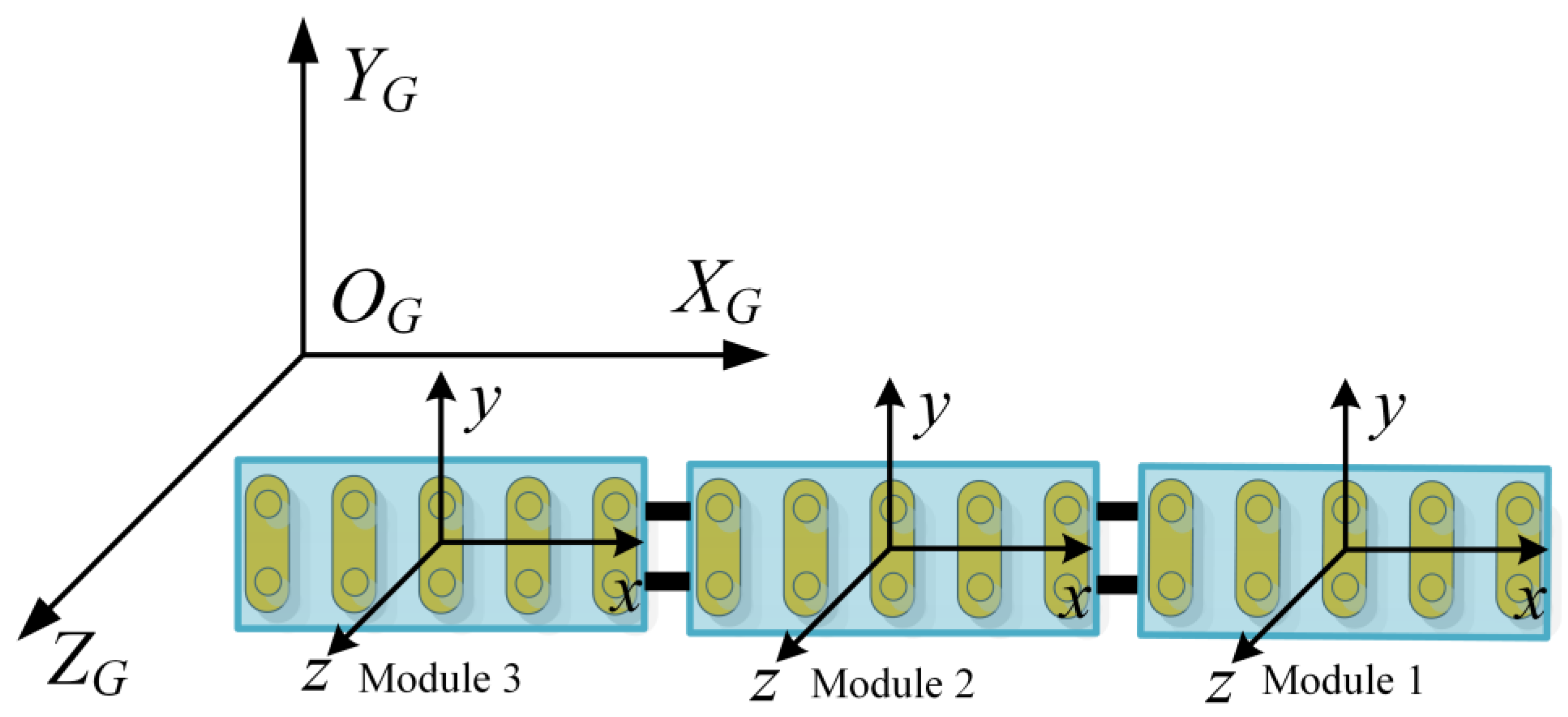
2.1. Hydrodynamic Model for VLFS Modules

In this section, the dynamics of a VLFS under the influence of environmental disturbances due to wind, waves, and current are presented. The dynamics of the mooring system are investigated using the lumped-mass method, and the dynamics of the connector are studied using the motion and geometric deformation method.

A global coordinate system is first defined as $\left(O_G-X_G{Y}_G{Z}_G\right)$ with origin $O_G$, as shown in Figure 1, which is parallel to the local coordinate systems $\left(x,y,z\right)$ of the VLFS module. The 6 degrees-of-freedom dynamics of a single module platform in the time domain can be described using the Cummins equations [22], which are defined in the local coordinate system $O-xyz$, fixed with respect to the mean position of each module. For a single module $i$ of a VLFS, its dynamics under the environmental disturbances are presented in the following equation:

$$\begin{array}{ll}\left(M_i+A_i\right){\ddot{x}}_i+{\int }_0^t{K}_i\left(t-\tau \right){\dot{x}}_i\left(\tau \right) d\tau +C_i{x}_i=& F_i^{wave}+F_i^{wind}+F_i^c+\\ & F_i^m+F_i^{connector}\end{array}$$

(1)

where $M_i$, $A_i$, $K_i$, and ${\mathbf{C}}_i\in {\mathbb{R}}^{6\times 6}$ are, respectively, the mass matrix of the module $i$, the constant infinite-frequency added-mass matrix, the matrix of retardation function, and the matrix of hydrostatic restoring forces. $x_i$, $F_i^{wave}$, $F_i^{wind}$, $F_i^c$, $F_i^m$, and $F_i^{connector}\in {\mathbb{R}}^{6\times 1}$ represent the 6-DOF motions, wave force, wind force, current force, mooring force, and connector force, respectively.

The dynamic equation of the mooring system is established, and the mooring force is solved using the finite element method. The calculation of the wind force employs empirical formulas.

The wave load effects on a VLFS module include both first-order wave excitation forces and second-order wave drift forces, which can be obtained using force response amplitude operators (RAOs) and quadratic transfer functions (QTFs), respectively. The connector force is caused by its deformation due to the out-of-sync motions of the adjacent modules, which are usually larger than the mooring force.

Given the frequency-dependent added mass, $A_i\left(\omega \right)$, and damping matrices, $B_i\left(\omega \right)$, we have the following:

$$\begin{array}{ll}\hspace{1em}{K}_i\left(t\right)& ={\displaystyle \frac{2}{\pi }}{\int }_0^t{B}_i\left(\omega \right)\mathrm{c}\mathrm{o}\mathrm{s}\left(\omega t\right) d\omega \\ A_i\left(\mathrm{\infty }\right)& =A_i\left(\omega \right)+{\displaystyle \frac{1}{\omega }}{\int }_0^t{K}_i\left(\tau \right)\mathrm{s}\mathrm{i}\mathrm{n}\left(\omega t\right) d\tau \end{array}$$

(2)

Upon establishing the parameters such as the mooring lines, the performance of the connector emerged as a critical factor impacting the motion response of the VLFS. Consequently, a comprehensive examination of the connector’s performance assumes significance. In the subsequent section, we present a numerical model designed for the analysis of VLFS connectors.

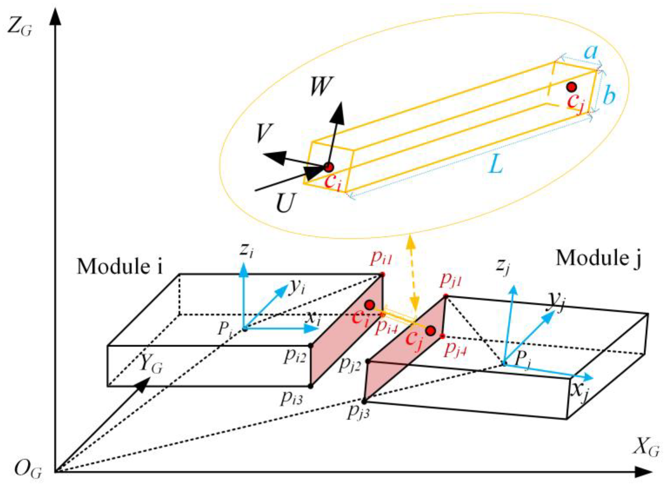
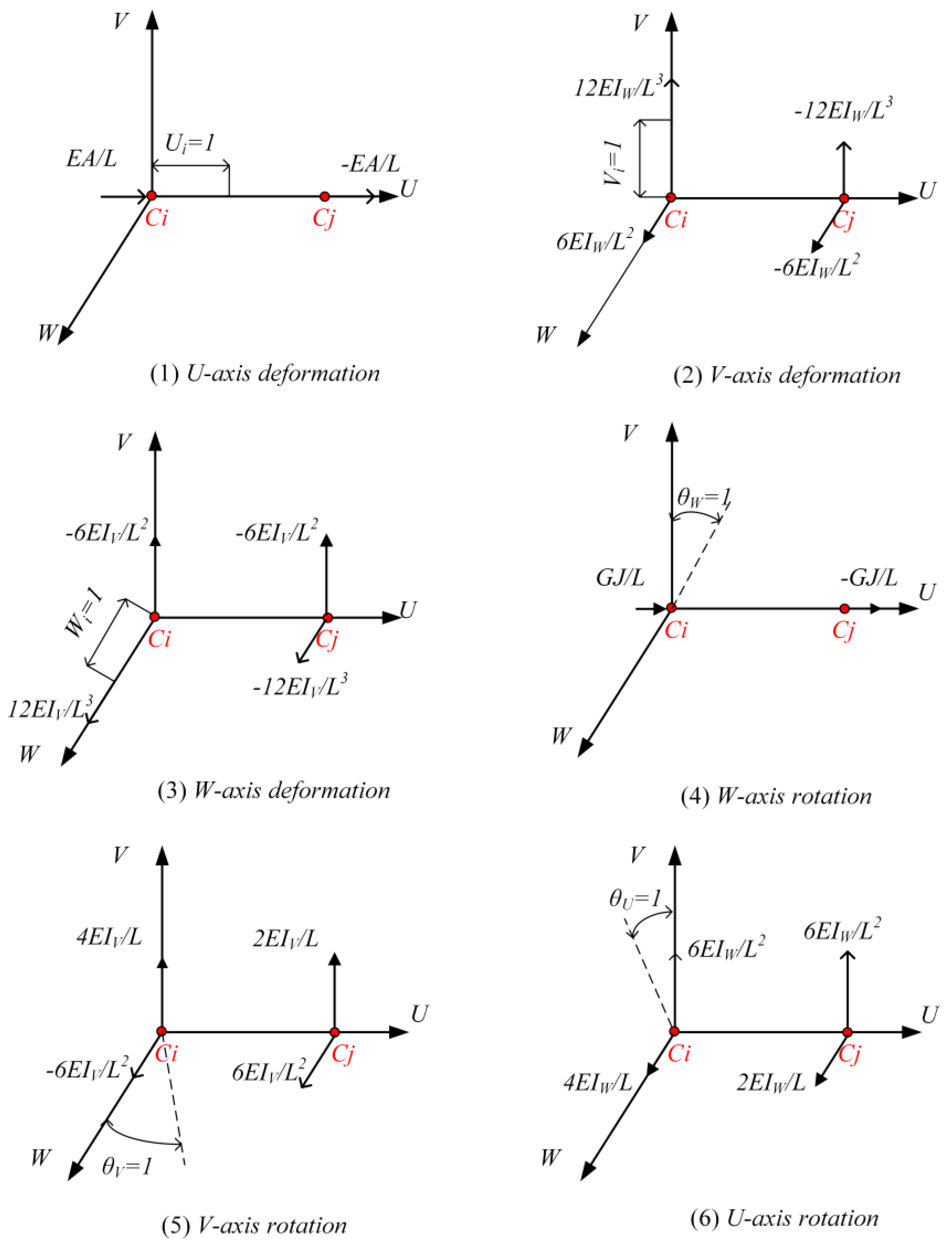
2.2. General Elastic Beam Model for VLFS Connectors

The uneven wave force applied to adjacent modules induces geometric deformation in a connector, which generates a corresponding restoring force that restricts the relative motion. To calculate the force in the connector, the geometric deformation of the connector and the 6-DOF motions of the modules must be determined. Figure 2 illustrates the center of gravity of two modules, denoted as $P_i$ and $P_j$, respectively. The two ends of the connector are rigidly connected to the module, while the connection points on the adjacent modules are referred to as $c_i$ and $c_j$. In the local coordinate system of the module, we have the following:

$$\begin{array}{c}{c}_i={\left[ \begin{array}{ccc}{x}_{ci}& y_{ci}& z_{ci}\end{array} \right]}^T\\ c_j={\left[ \begin{array}{ccc}{x}_{cj}& y_{cj}& z_{cj}\end{array} \right]}^T\end{array}$$

(3)

The 6-DOF motions of module $i$ and module $j$ are, respectively, ${\mathbf{x}}_{\mathbf{i}}$ and ${\mathbf{x}}_{\mathbf{j}}$, and we have the following:

$$\begin{array}{c}{\mathbf{x}}_{\mathbf{i}}={\left[\begin{array}{ccccc}{x}_i& y_i& z_i{\alpha }_i& {\beta }_i& {\gamma }_i\end{array}\right]}^T\\ {\mathbf{x}}_{\mathbf{j}}={\left[\begin{array}{ccccc}{x}_j& y_j& z_j{\alpha }_j& {\beta }_j& {\gamma }_j\end{array}\right]}^T\end{array}$$

(4)

The connector’s structure is usually very complex, and it is difficult to fully simulate all of its mechanical properties. To simplify the model, an elastic bar with stiffness and damping is used to simulate the connector in this paper. At point $c_i$, a connector coordinate system, $UVW,$ is established, as depicted in Figure 2. This coordinate system is parallel to module $i$’s local coordinate system. The connector is rigidly connected to the VLFS module.

The displacement and force at both ends of the elastic bar can be expressed in the coordinate system $c_i-UVW$, as follows:

$$\begin{array}{c}{\overline{\delta }}_{ijc}={\left[\begin{array}{cccccccccccc}{\overline{u}}_i& {\overline{v}}_i& {\overline{w}}_i& {\overline{\theta }}_{ui}& {\overline{\theta }}_{vi}& {\overline{\theta }}_{wi}& {\overline{u}}_j& {\overline{v}}_j& {\overline{w}}_j& {\overline{\theta }}_{uj}& {\overline{\theta }}_{vj}& {\overline{\theta }}_{wj}\end{array}\right]}^T\\ {\overline{F}}_{ijc}={\left[\begin{array}{cccccccccccc}{\overline{F}}_{xi}& {\overline{F}}_{yi}& {\overline{F}}_{zi}& {\overline{M}}_{xi}& {\overline{M}}_{yi}& {\overline{M}}_{zi}& {\overline{F}}_{xj}& {\overline{F}}_{yj}& {\overline{F}}_{zj}& {\overline{M}}_{xj}& {\overline{M}}_{yj}& {\overline{M}}_{zj}\end{array}\right]}^T\end{array}$$

(5)

where $\overline{u}$, $\overline{v},$ and $\overline{w}$ are the elastic end-bar displacements, and ${\overline{\theta }}_u$, ${\overline{\theta }}_v$, and ${\overline{\theta }}_w$ are the elastic end-bar rotation angles. Correspondingly, ${\overline{F}}_x$, ${\overline{F}}_y$, and ${\overline{F}}_z$ are the forces of the elastic bar in the direction of $UVW$, and ${\overline{M}}_x$, ${\overline{M}}_y$, and ${\overline{M}}_z$ are the torque at the end of the bar.

The deformations of the elastic bar can be decomposed into tension, compression, shear, bending, and torsion deformation. In Figure 3, the relationship between the end force and displacement of the elastic bar is illustrated when a unit displacement occurs at end $i$. As shown in Figure 3(1), it depicts the force at end $i$ when the displacement component in the U-direction is 1, while the other components are all zero. By the same token, Figure 3(2) to Figure 3(6) illustrate the force conditions in the remaining several directions.

The direction of the moment of the couple and angular displacement is indicated by sharp, filled arrows following the right-hand rule, while the direction of the force and linear displacement is represented by an open arrow. $A$ represents the cross-section of the elastic bar, $L$ is the length of the bar, $E$ denotes the Young’s modulus, and $G$ represents the shear modulus. Additionally, $I_U$, $I_V$, and $I_W$ refer to the inertia moments of the elastic bar around the $U$, $V$, and $W$ axes, respectively.

The stiffness matrix of the connector, denoted as ${\overline{\mathbf{K}}}_{\mathbf{c}}$, is defined in the $UVW$ coordinate system.

$$\begin{array}{r}{\overline{\mathbf{K}}}_{\mathbf{c}}=\left[\begin{array}{c}\begin{array}{cccccccccccc}{\displaystyle \frac{EA}{L}}& & & & & & & & & & & \\ 0& {\displaystyle \frac{12E{I}_W}{L^3}}& & & & & & & & & & \\ 0& 0& {\displaystyle \frac{12E{I}_V}{L^3}}& & & & & & & & & \\ 0& 0& 0& {\displaystyle \frac{G{I}_U}{L}}& & & & & symmetry& & & \\ 0& 0& {\displaystyle \frac{-6E{I}_V}{L^2}}& 0& {\displaystyle \frac{4E{I}_V}{L}}& & & & & & & \\ 0& {\displaystyle \frac{6E{I}_W}{L^2}}& 0& 0& 0& {\displaystyle \frac{4E{I}_W}{L}}& & & & & & \\ {\displaystyle \frac{-EA}{L}}& 0& 0& 0& 0& 0& {\displaystyle \frac{-EA}{L}}& & & & & \\ 0& {\displaystyle \frac{-12E{I}_W}{L^3}}& 0& 0& 0& {\displaystyle \frac{-6E{I}_W}{L^2}}& 0& {\displaystyle \frac{12E{I}_W}{L^3}}& & & & \\ 0& 0& {\displaystyle \frac{-12E{I}_V}{L^3}}& 0& {\displaystyle \frac{6E{I}_V}{L^2}}& 0& 0& 0& {\displaystyle \frac{12E{I}_V}{L^3}}& & & \\ 0& 0& 0& {\displaystyle \frac{-G{I}_U}{L}}& 0& 0& 0& 0& 0& {\displaystyle \frac{G{I}_U}{L}}& & \\ 0& 0& {\displaystyle \frac{-6E{I}_V}{L^2}}& 0& {\displaystyle \frac{2E{I}_V}{L}}& 0& 0& 0& {\displaystyle \frac{6E{I}_V}{L^2}}& 0& {\displaystyle \frac{4E{I}_V}{L}}& \\ 0& {\displaystyle \frac{6E{I}_W}{L^2}}& 0& 0& 0& {\displaystyle \frac{2E{I}_W}{L}}& 0& {\displaystyle \frac{-6E{I}_W}{L^2}}& 0& 0& 0& {\displaystyle \frac{4E{I}_W}{L}}\end{array}\end{array}\right]\end{array}$$

(6)

In this context, we have the following definitions:

$$I_U=ab{L}^2, I_V=a{b}^3/12, I_W=a^{3}b/12$$

(7)

where $a$ and $b$ are the dimensions of the cross-section, and $L$ is the length of the connector.

In the local coordinate system of module $i$, the forces acting on the ends of the elastic bar are as follows:

$$\begin{array}{r}{\overline{\mathbf{F}}}_{\mathbf{i}\mathbf{j}\mathbf{c}}\left(\mathbf{t}\right)={\overline{\mathbf{K}}}_{\mathbf{c}}\cdot {\overline{\mathsf{\delta }}}_{\mathbf{i}\mathbf{j}\mathbf{c}}\end{array}$$

(8)

The forces acting on end $c_i$ of the elastic bar in the local coordinate system of module $i$ are as follows:

$$\begin{array}{r}{\mathbf{F}}_{ic}\left(t\right)=\left[\begin{array}{cc}{I}_{6\times 6}& 0_{6\times 6}\end{array}\right]\cdot {\overline{\mathbf{F}}}_{\mathbf{i}\mathbf{j}\mathbf{c}}\left(\mathbf{t}\right)\end{array}$$

(9)

Now, we have the restoring force generated by the stiffness of the connector. However, it is important to note that the damping effect of the connector cannot be neglected. The connector not only provides constraints among the modules but also dissipates a significant amount of structural kinetic energy during its operation. At present, there are various methods to incorporate damping in engineering applications. One commonly used damping model is Rayleigh damping, known for its simplicity and convenience in structural dynamic analysis. Rayleigh damping is a form of viscous damping that is proportional to a linear combination of the mass and stiffness. The damping matrix, denoted as $C_c$, can be expressed as follows:

$$\begin{array}{r}{\mathbf{C}}_c=\mu {\mathbf{M}}_{\mathbf{c}}+\lambda {\overline{\mathbf{K}}}_{\mathbf{c}}\end{array}$$

(10)

where ${\mathbf{M}}_{\mathbf{c}}$ and ${\overline{\mathbf{K}}}_{\mathbf{c}}$ are the connector’s mass and stiffness matrices, respectively. The damping matrix, $C_c$, is determined by the stiffness proportional damping constant, $\mu$, and the mass proportional damping constant, $\lambda$.

Rayleigh damping is commonly utilized in structural analysis due to its mathematical simplicity and ability to represent internal structural damping. However, one drawback of Rayleigh damping is that the achieved damping ratio, $\xi$, varies with the frequency of the response. The stiffness proportional term in Rayleigh damping contributes damping that is linearly proportional to the response frequency, while the mass proportional term contributes damping that is inversely proportional to the response frequency. The values of $\mu$ and $\lambda$, which are the stiffness and mass proportional damping constants, respectively, are determined by selecting the fractions of critical damping at the first two distinct non-zero frequencies.

Considering the stiffness and damping of the connector, the forces exerted on point $c_i$ of the module by the connector in the local coordinate system of module $i$ are as follows:

$$\begin{array}{r}{\mathbf{F}}_{\mathbf{i}\mathbf{c}}\left(\mathbf{t}\right)=-\left[\begin{array}{cc}{I}_{6\times 6}& 0_{6\times 6}\end{array}\right]\cdot \left({\overline{\mathbf{K}}}_{\mathbf{c}}{\overline{\mathsf{\delta }}}_{\mathbf{i}\mathbf{j}\mathbf{c}}+{\mathbf{C}}_{\mathbf{c}}{\dot{\overline{\mathsf{\delta }}}}_{\mathbf{i}\mathbf{j}\mathbf{c}}\right)\end{array}$$

(11)

$${\overline{\mathbf{F}}}_{\mathbf{i}\mathbf{c}}\left(\mathbf{t}\right)=\left[\begin{array}{cccccc}1& 0& 0& 0& 0& 0\\ 0& 1& 0& 0& 0& 0\\ 0& 0& 1& 0& 0& 0\\ 0& 0& y_{ci}& 1& 0& 0\\ 0& 0& {-x}_{ci}& 0& 1& 0\\ {-y}_{ci}& x_{ci}& 0& 0& 0& 1\end{array}\right]\cdot {\mathbf{F}}_{\mathbf{i}\mathbf{c}}\left(\mathbf{t}\right)$$

(12)

3. Validation of the Proposed Connector Mechanical Model

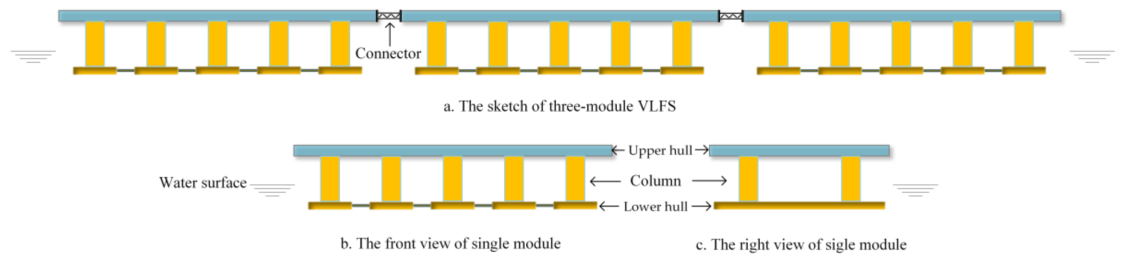
3.1. Parameters of the VLFS

To verify the applicability and accuracy of the proposed numerical model, physical model tests were conducted. The case studies focused on a VLFS composed of three identical semi-submerged platforms connected in a series via flexible connectors, as depicted in Figure 4 and Figure 5. Each semi-submerged platform comprises an upper hull, ten columns, and five lower hulls. The geometric and structural parameters of the semi-submerged platform are provided in

Table 1. Main parameters of the VLFS’s single module.

Term	Parameter	VLFS	Term	Parameter	VLFS
Upper hull	Length/m	300	Inertia radius	Roll/m	28.47
	Width/m	100		Pitch/m	86.31
	Height/m	6		Yaw/m	89.77
Lower hull	Length/m	96	Others	Draught/m	12
	Width/m	30		Displacement/t	93,614
	Height/m	5		Center of gravity/m	12
Columns	Cross-section	Circle
	Radius/m	9
	Height/m	16

.

The flexible connector was represented by an elastic bar model, and its equivalent parameters were determined through mechanical testing on a dedicated test platform. These parameters are presented in

Table 2. Connector parameters in the numerical and experimental test.

Connector	Young’s Modulus	Shear Modulus	Cross-Section		Length
	E/MPa	G/MPa	a/m	b/m	Lc/m
-	50	25	5	5	6

. By utilizing the provided values for the Young’s modulus, shear modulus, length, and cross-section parameters, the stiffness matrix of the flexible connector can be calculated using Equation (10).

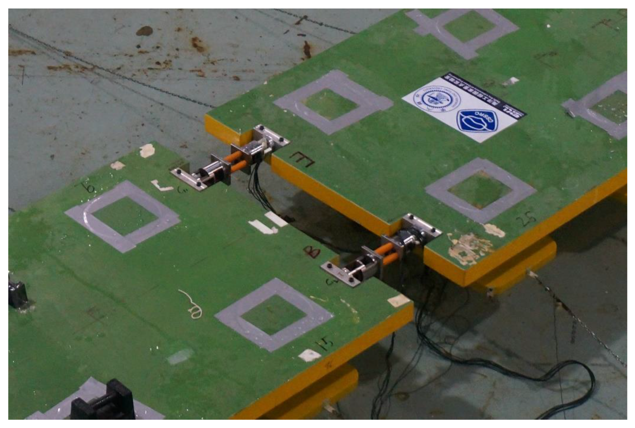
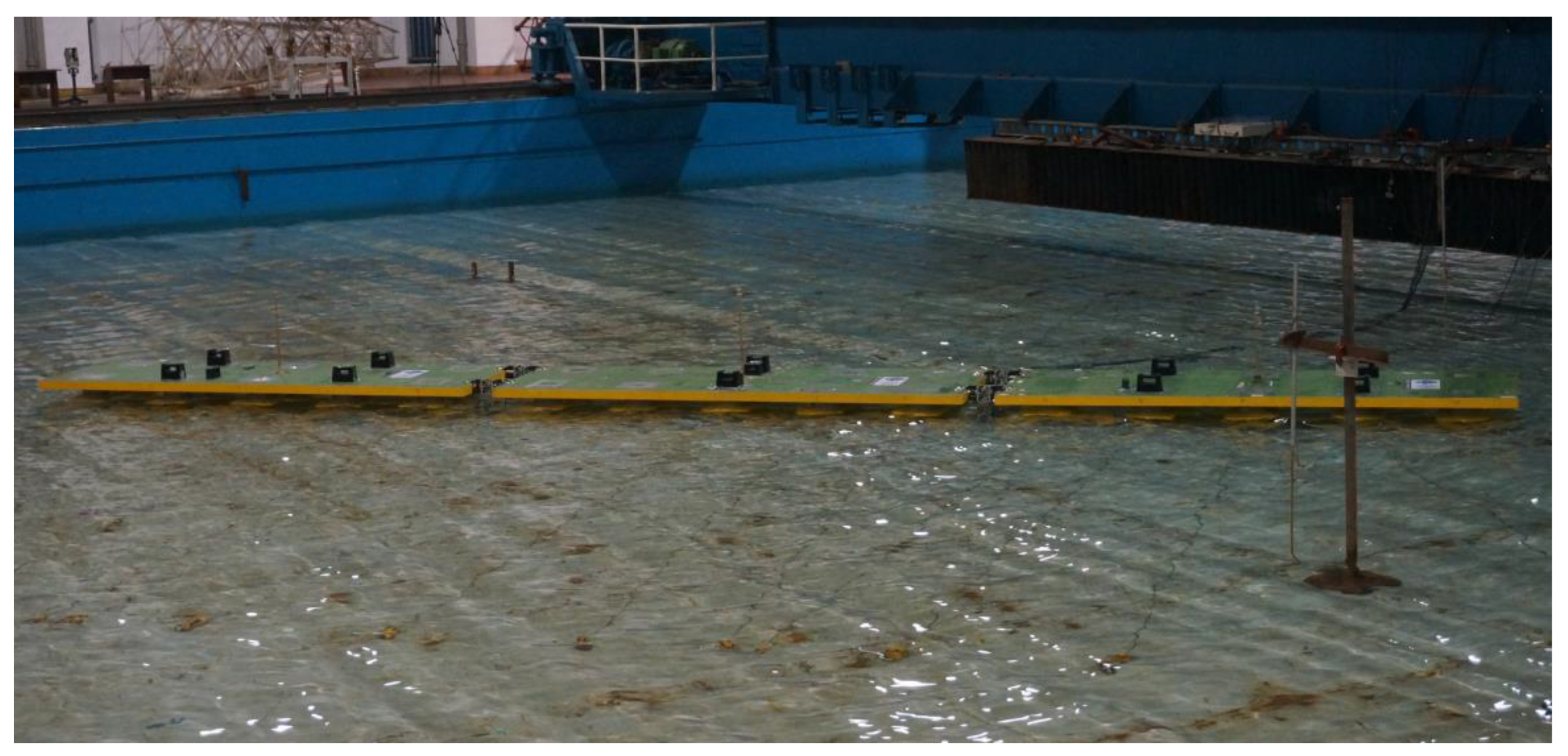
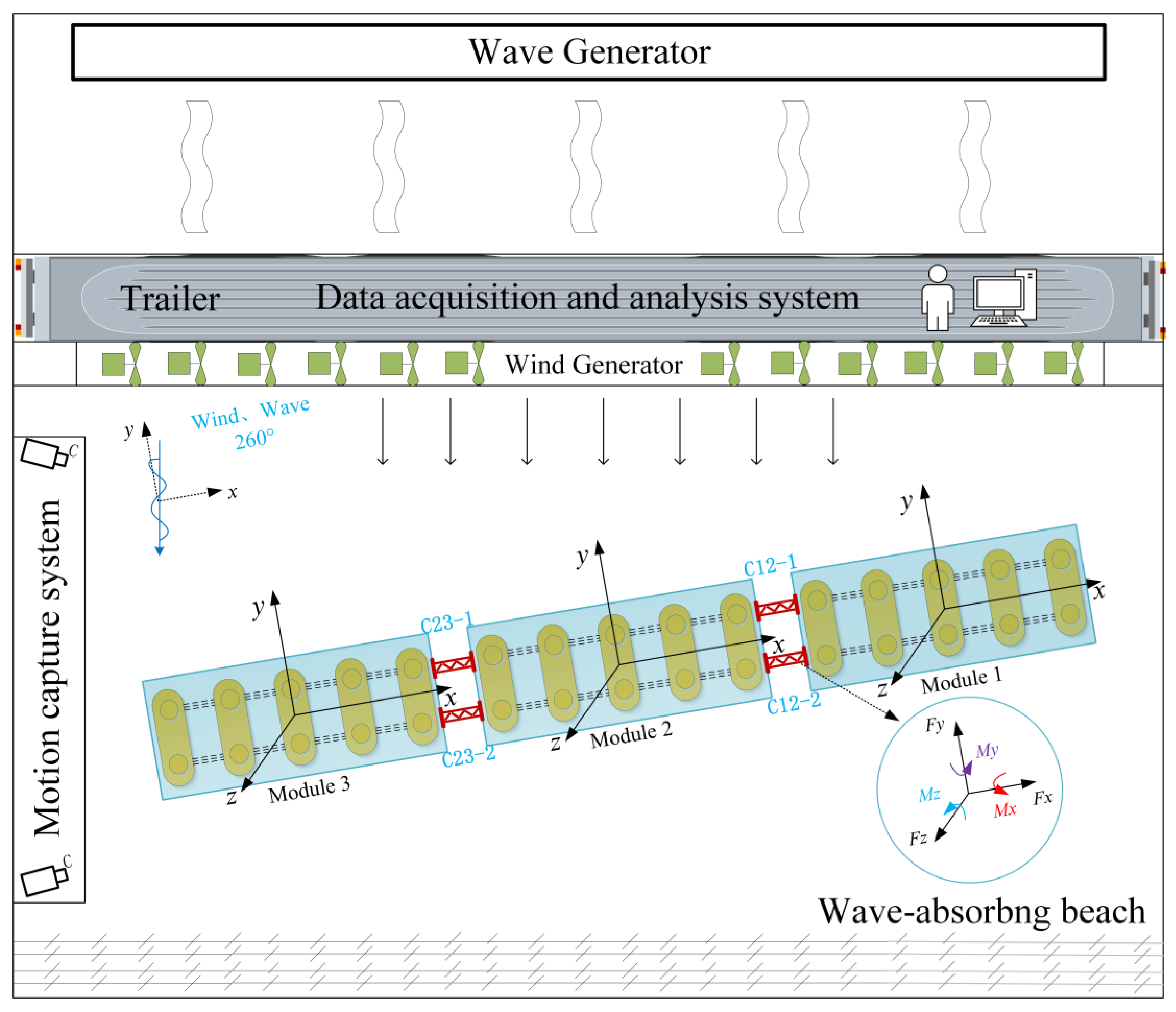
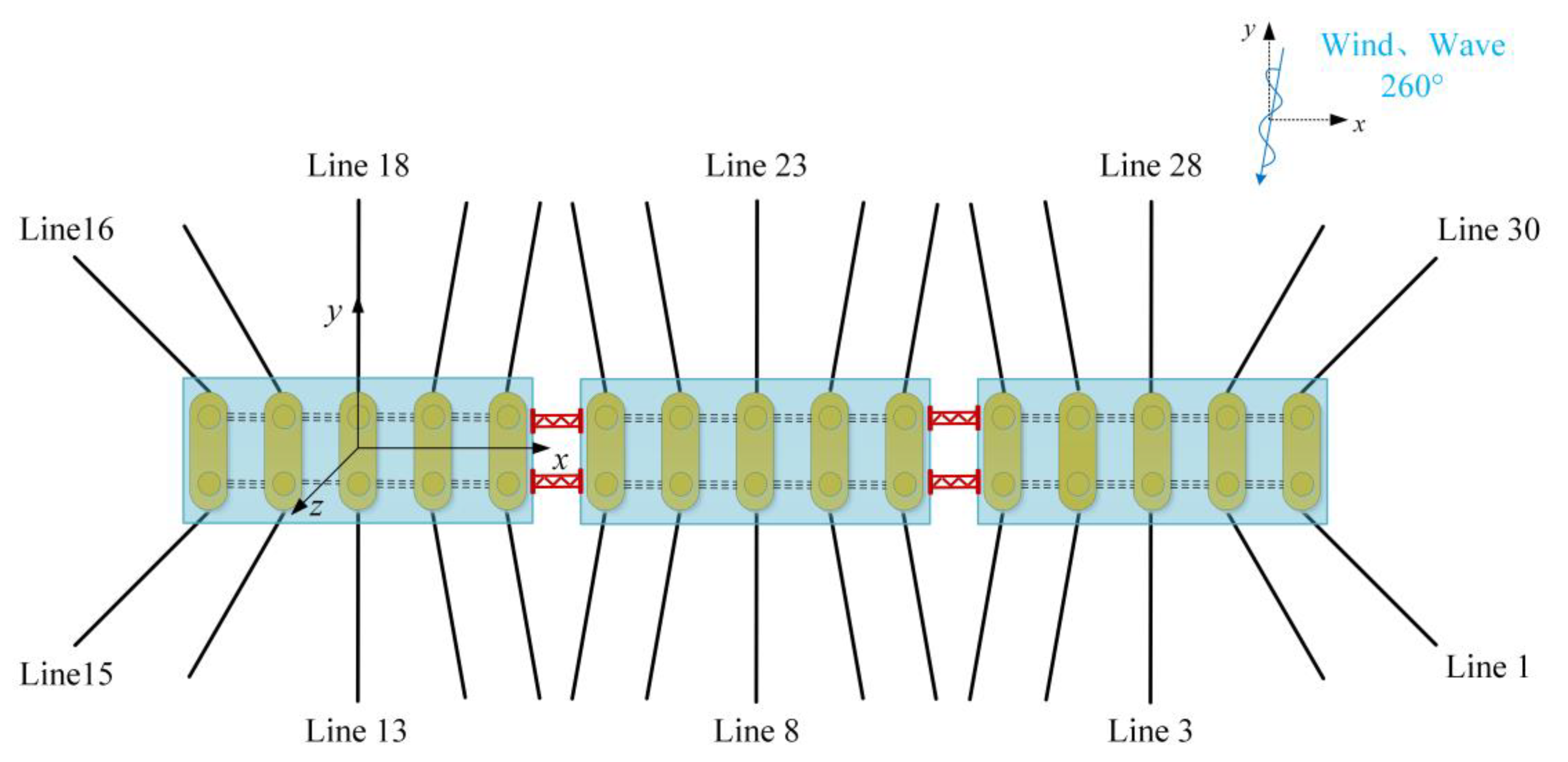
3.2. Setting of the Experimental Parameters

The physical model test was carried out in the ocean engineering basin at the State Key Laboratory of Ocean Engineering, Shanghai Jiao Tong University, as shown in Figure 6. The ocean engineering basin has a main scale of 50 m in length and 30 m in width. The water depth of the basin can be adjusted within a range of 0 m to 5 m.

Table 3. Environment conditions.

No.	Significant Wave	Spectrum Peak	Wind
	Height [m]	Period [s]	[m/s]
1	3	7.48	10
2	5	9.66	36

provides the environmental parameters for inhomogeneous wave and wind conditions in the vicinity of the South China Sea reef. The No. 1 wave condition, with a height of 3 m, represents the operational condition of the VLFS, while the No. 2 wave condition, with a height of 5 m, represents the condition when the connectors are unlocked. The target wave was generated using a wave generator and validated prior to the model’s test. Similarly, the target wind was generated using an axial flow fan and also validated prior to the model’s test.

Figure 7 illustrates the overall layout of the VLFS model in the ocean engineering basin. It includes the direction of the environmental forces, the coordinate system of each module, the arrangement of the connectors, and a component diagram of the connectors. In total, there were four connectors between adjacent VLFS modules, namely, C12-1, C12-2, C23-1, and C23-2.

During the model’s test, the six degrees-of-freedom (6-DOF) motions of the VLFS were captured using an optical motion capture system (called the Marine Trak system). The motion measurement’s accuracy was 1 mm. Additionally, the forces acting on the mooring lines and connectors were measured using force sensors.

Figure 8 shows the overall layout of the VLFS mooring system. The mooring system consists of a total of 30 mooring lines.

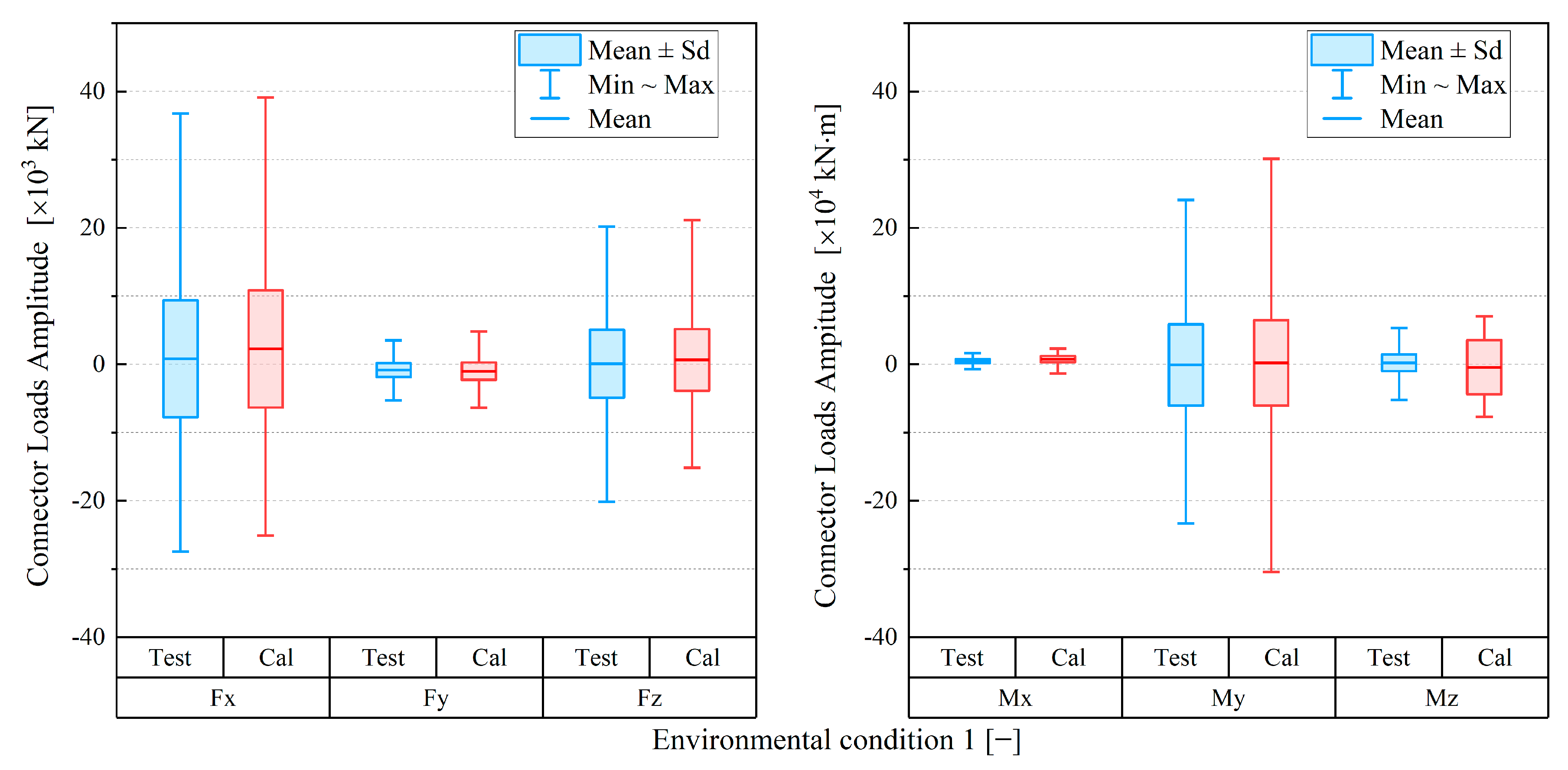
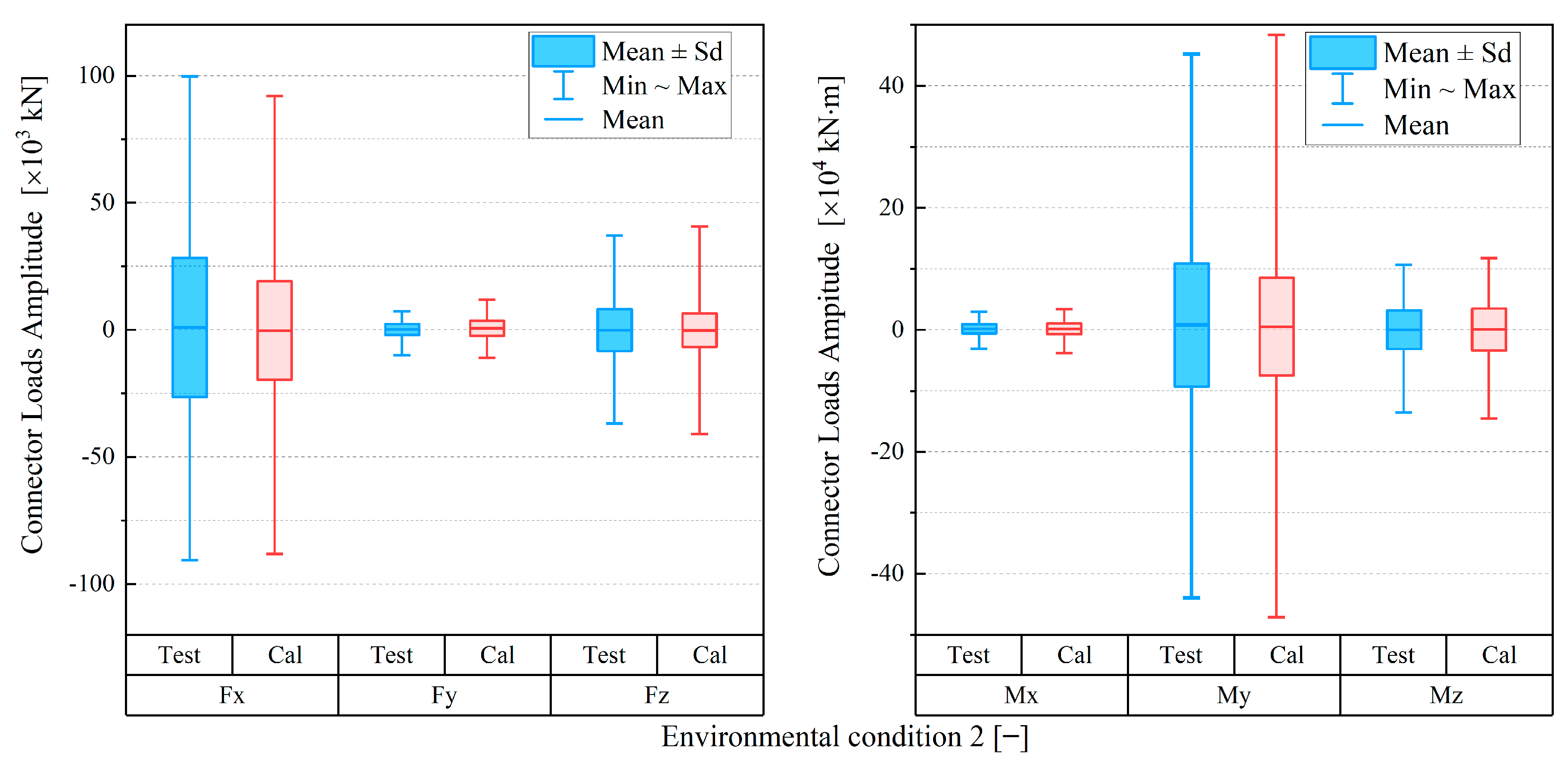
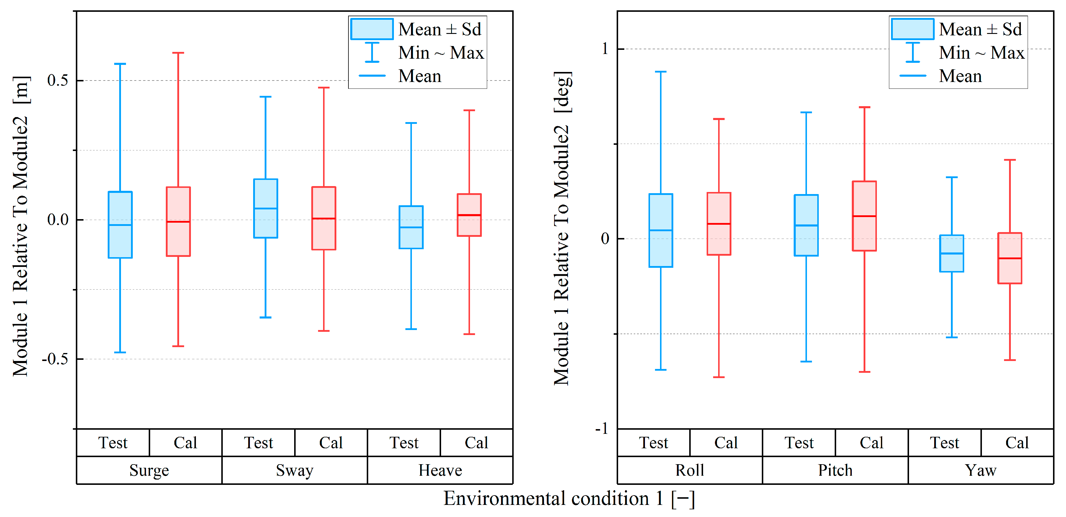
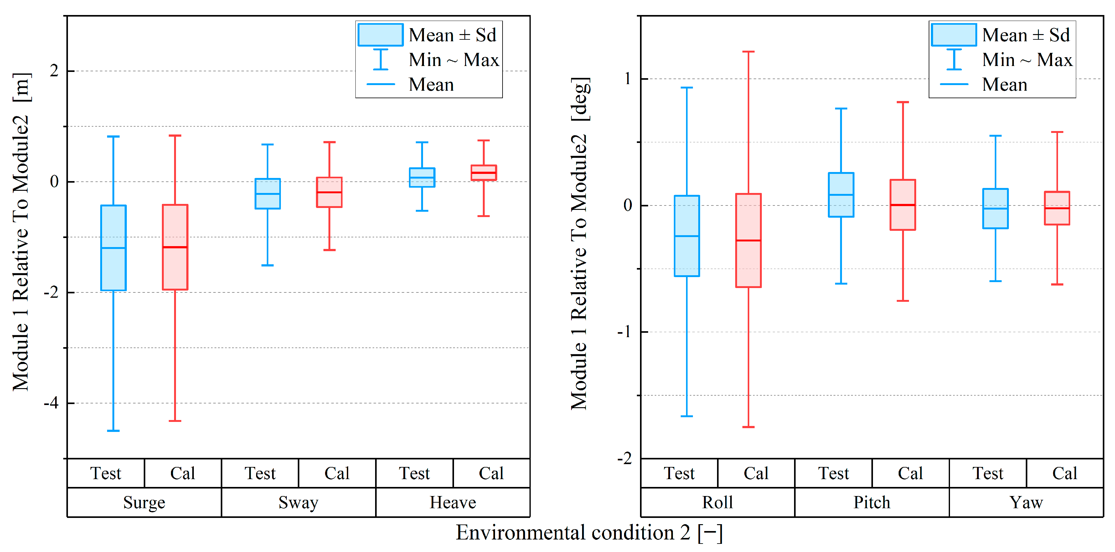
3.3. Verification Results

The physical model test was conducted in the ocean engineering basin to validate the accuracy and rationality of the numerical simulation model. As depicted in Figure 9 and Figure 10, a comparison was made between the loads acting on connector C12-1 obtained from the numerical simulation and the experimental tests. The results indicate a close agreement in terms of the peak loads experienced by the connector in all directions.

As illustrated in Figure 11 and Figure 12, a comparison was conducted between the relative motion of the VLFS modules obtained from the numerical simulation and the experimental tests. The results demonstrate a favorable agreement in terms of the relative motions among the VLFS modules. This suggests that the numerical simulation can serve as a valuable research tool, providing guidance for conducting sensitivity analyses and optimization of the connector parameters.

Based on the verifications conducted, it was determined that the proposed numerical model is suitable for analyzing the dynamic responses of connectors and VLFS systems. In the subsequent section, the focus is on the study of the connector parameters using the numerical simulation model.

4. Connector Parameter Analysis and Optimization

The geometrical and structural parameters of the connector can have a significant impact on the dynamic response of the VLFS modules. However, studying these parameters often requires a large number of numerical simulations and corresponding experiments. To reduce the number of tests required, the orthogonal experiment method is employed. This method combines probability theory and mathematical statistics to systematically and efficiently explore the effects of multiple parameters on the dynamic response of the VLFS modules. By using this method, it is possible to obtain valuable insight while minimizing the number of numerical and experimental tests needed.

In this paper, the research on the connector parameters is essentially a complicated multi-objective optimization problem. The decision variable primarily consists of the stiffness matrix of the connector, while the objective function encompasses both the motion parameters of the VLFS and the loads imposed on the connector itself. The internal parameters of the connector stiffness matrix, being the decision variable, are intricate, and hence, specific key parameters were selected for investigation. Furthermore, the objective function is a multidimensional function. For the three-module VLFS, each module exhibits 6-DOF in motion, and each connector is subjected to forces and torque in all directions. To simplify the problem, the objective functions, motion amplitudes, and connector loads are discussed and normalized as performance criteria for the connector, based on the requirements of the VLFS application scenario.

4.1. VLFS Motion Normalization

VLFSs serve various purposes, such as floating airports, floating landing platforms, and bridges at sea. It is crucial to ensure deck flatness in small VLFS modules, which can be achieved through the optimization of connector parameters. However, examining the 6-DOF motions of each module individually during the optimization process can result in a complicated problem with multiple dimensions. Additionally, relying solely on the 6-DOF motion amplitudes of the VLFS module may not accurately depict the flatness of the VLFS deck, particularly the relative displacement changes at the module joints. To address this, the relative changes in the position and attitude between adjacent faces of the modules were normalized to illustrate the flatness of the VLFS deck.

As shown in the Figure 2, there exist two modules denoted by their respective center of gravity points, as follows: $P_i$ and $P_j$. The position of the two modules can be expressed in the global coordinate system as follows:

$$\begin{array}{rr}{\mathbf{P}}_{\mathbf{i}}& ={\left[\begin{array}{ccc}{X}_i& Y_i& Z_i\end{array}\right]}^{\mathrm{T}}\\ {\mathbf{P}}_{\mathbf{j}}& ={\left[\begin{array}{ccc}{X}_j& Y_j& Z_j\end{array}\right]}^{\mathrm{T}}\end{array}$$

(13)

The analysis focused on the relative changes in the position and attitude between the adjacent faces of the modules, namely, $p_{i1}{p}_{i2}{p}_{i3}{p}_{i4}$ and $p_{j1}{p}_{j2}{p}_{j3}{p}_{j4}$. To establish the motion relationship between these faces, we initially select points at the four corners of each face. The positions of these eight points on the two faces can be determined based on the geometric dimensions of the module. For instance, the coordinates $p_{i1}$ and $p_{j1}$ can be expressed in the local coordinate systems of the respective modules as follows:

$$\begin{array}{ll}{\mathbf{p}}_{\mathbf{i}1}& ={\left[\begin{array}{ccc}{x}_{i1}& y_{i1}& z_{i1}\end{array}\right]}^{\mathrm{T}}={\left[\begin{array}{ccc}150& 50& 15\end{array}\right]}^{\mathrm{T}}\\ {\mathbf{p}}_{\mathbf{j}1}& ={\left[\begin{array}{ccc}{x}_{j1}& y_{j1}& z_{j1}\end{array}\right]}^{\mathrm{T}}={\left[\begin{array}{ccc}-150& 50& 15\end{array}\right]}^{\mathrm{T}}\end{array}$$

(14)

The coordinates of point $p_{i1}$ and $p_{j1}$ can be transformed to the global coordinate system using the coordinate transformation matrices ${\mathbf{T}}_{\mathbf{i}}$ and ${\mathbf{T}}_{\mathbf{i}}$, respectively. Subsequently, by adding the coordinates of the module’s center of gravity, the coordinates of $p_{i1}$ and $p_{j1}$ in the global coordinate system can be obtained. Mathematically, they can be expressed as follows:

$$\begin{array}{rr}{\mathbf{P}}_{\mathbf{i}1\_\mathbf{g}\mathbf{l}\mathbf{o}\mathbf{b}\mathbf{a}\mathbf{l}}& ={\left[\begin{array}{ccc}{X}_{i1}& Y_{i1}& Z_{i1}\end{array}\right]}^{\mathrm{T}}={\mathbf{T}}_{\mathbf{i}}\cdot {\mathbf{p}}_{\mathbf{i}1}+{\mathbf{P}}_{\mathbf{i}}\\ {\mathbf{P}}_{\mathbf{j}1\_\mathbf{g}\mathbf{l}\mathbf{o}\mathbf{b}\mathbf{a}\mathbf{l}}& ={\left[\begin{array}{ccc}{X}_{j1}& Y_{j1}& Z_{j1}\end{array}\right]}^{\mathrm{T}}={\mathbf{T}}_{\mathbf{j}}\cdot {\mathbf{p}}_{\mathbf{j}1}+{\mathbf{P}}_{\mathbf{j}}\end{array}$$

(15)

where ${\mathbf{P}}_{\mathbf{i}1\_\mathbf{g}\mathbf{l}\mathbf{o}\mathbf{b}\mathbf{a}\mathbf{l}}$ and ${\mathbf{P}}_{\mathbf{j}1\_\mathbf{g}\mathbf{l}\mathbf{o}\mathbf{b}\mathbf{a}\mathbf{l}}$ represent the coordinates of $p_{i1}$ and $p_{j1}$ in the global coordinate system, respectively. ${\mathbf{T}}_{\mathbf{i}}$ and ${\mathbf{T}}_{\mathbf{i}}$ are the coordinate transformation matrices, and $P_i$ and $P_j$ are the coordinates of the center of gravity of the respective modules.

Similarly, we can determine the coordinates of the other points in the global coordinate system. Once the coordinates of these points are obtained, the changes in the relative position and attitude of the adjacent modules can be expressed as follows:

$$\begin{array}{r}{D}_{ij}={\sum }_{n=1}^4\left||X_{in}-X_{jn}|+|Y_{in}-Y_{jn}|+|Z_{in}-Z_{jn}|-d\right|\end{array}$$

(16)

In the equation, the term $d$ represents the initial spacing between adjacent modules. The term $D_{ij}$ is a normalized objective function that encompasses all 6-DOF motions. It accurately reflects the influence of different connector decision variables on the motion response performance of the VLFS. The absolute value signs in the equation ensure that the criterion takes into account all variations in the relative position in all directions. When the modules remain stationary relative to each other, the objective function, $D_{ij}$, is equal to 0 m. As the amplitude of the relative motion among the modules increases, the objective function, $D_{ij}$, increases. For a three-module VLFS, the largest value of $D_{ij}$, denoted as $D_{max}$, is selected as the final objective function. A smaller value of the objective function, $D_{max}$, indicates a better performance by the connector.

$$\begin{array}{r}{D}_{max}=\mathrm{m}\mathrm{a}\mathrm{x}\left\{D_{12},D_{23}\right\}\end{array}$$

(17)

4.2. Connector Load Normalization

When selecting the appropriate connector parameters based on $D_{max}$, a screening method for the connector parameters is developed using the connector load selection criteria. This method aims to minimize manufacturing difficulties and improve the service life of the connector. The screening criteria determine the optimal parameter scheme by considering the connector with smaller loads. Therefore, the objective functions are proposed, which include connector loads and moments in the $x$, $y$, and $z$ directions.

At the end point of the connector, there is the connector coordinate system $UVW$, as shown in Figure 2. Since the connection point of the connector and the VLFS module is rigidly connected and the 6-DOF motions are fully constrained, the coordinate system is parallel to module $i$’s local coordinate system. The loads acting on the connector are multidimensional and encompass the forces and moments in various directions. Under connector coordinate system $UVW$, the force at both ends of the elastic bar can be expressed as follows:

$$\begin{array}{r}{\overline{\mathbf{F}}}_{\mathbf{i}\mathbf{c}}={\left[\begin{array}{cccccc}{\overline{F}}_{xi}& {\overline{F}}_{yi}& {\overline{F}}_{zi}& {\overline{M}}_{xi}& {\overline{M}}_{yi}& {\overline{M}}_{zi}\end{array}\right]}^{\mathrm{T}}\end{array}$$

(18)

Two objective functions are defined, which represent the maximum force and torque on the connector, respectively, as follows:

$$\begin{array}{ll}{F}_{max}& =\mathrm{m}\mathrm{a}\mathrm{x}\left\{F_x,F_y,F_z\right\}\\ M_{max}& =\mathrm{m}\mathrm{a}\mathrm{x}\left\{M_x,M_y,M_z\right\}\end{array}$$

(19)

In the process of the connector parameters’ sensitivity analysis and optimization, we considered the relative motion among the modules to have higher priority than the connector load. However, there is still a dynamic balance between them. It is not advisable to optimize one side blindly while ignoring the other.

4.3. Setting of the Orthogonal Analysis Strategy

The orthogonal experiment method was employed to analyze the impact of the connector parameters on the dynamic response of the VLFS. This method proves to be an efficient tool in engineering, as it requires a minimum number of numerical simulations and corresponding experiments. However, before designing the orthogonal tests, it is crucial to determine the key parameters that will be investigated.

Based on the analysis of the previous model tests, it can be concluded that the stiffness matrices play a crucial role in influencing the motion response of the VLFS, as well as the loads on the connectors. When considering numerical models for connectors, the stiffness matrix is determined by parameters such as the Young’s modulus, shear modulus, and cross-sectional parameters. In the design of the orthogonal simulation tests, the key parameters of the connector stiffness matrix were the Young’s modulus (E), shear modulus (G), and cross-sectional parameters (a, b). By utilizing these factors, a stiffness matrix can be derived using Formula (6). Subsequently, the effects of the connector stiffness matrix on the motion response of the VLFS and the loads on the connectors can be studied.

According to the experimental tests, three levels for each key factor of the connector are proposed. In this way, there are altogether $81$ connectors with different parameters. In addition, two different waves should be used in the test, so there are altogether $162$ cases. The number of cases can be too computationally demanding. The experiment can be designed according to a four-factor, and three-level orthogonal table (

Table 4. Factor level of the flexible connector orthogonal test scheme.

No.	Young’s Modulus	Shear Modulus	Cross-Section		Length
	E [MPa]	G [MPa]	a [m]	b [m]	Lc [m]
1	10	5	4	4	6
2	10	50	4.5	4.5	6
3	10	25	5	5	6
4	50	25	4.5	4	6
5	50	5	5	4.5	6
6	50	50	4	5	6
7	100	50	5	4	6
8	100	25	4	4.5	6
9	100	5	4.5	5	6

). The four-factor and three-level orthogonal experiment regarded the relative motion amplitude (objective function, $D_{max}$) and connector loads ($F_{max}$ and $M_{max}$) as indicators for evaluating the connector performance [23].

The equivalent parameters were determined according to the connector’s structural form and material characteristics; however, this does not mean that there must be a certain material with these properties.

4.4. Results and Discussion

The calculated dynamic response characteristics of the VLFS equipped with different connectors under environmental forces, as well as the objective function statistics, are shown in total in

Table 5. Objective functions for different connectors.

Connector	${\mathit{D}}_{\mathit{m}\mathit{a}\mathit{x}}$ (m)		${\mathit{F}}_{\mathit{m}\mathit{a}\mathit{x}}$ ($\times {10}^3 \mathbf{k}\mathbf{N}$)		${\mathit{M}}_{\mathit{m}\mathit{a}\mathit{x}}$ ($\times {10}^4 \mathbf{k}\mathbf{N} \mathbf{m}$)
	Env_Con_1	Env_Con_2	Env_Con_1	Env_Con_2	Env_Con_1	Env_Con_2
1	2.37	3.11	5.33	17.57	30.99	63.77
2	2.91	3.59	8.53	22.92	33.96	88.58
3	2.77	3.11	7.12	20.02	36.42	95.27
4	2.19	2.26	8.92	19.76	28.91	68.78
5	2.3	2.47	9.01	21.8	34.24	82.68
6	2.01	2.25	8.66	24.8	32.11	72.19
7	1.47	1.58	11.02	25.58	38.13	75.92
8	1.68	1.77	10.73	27.06	30.97	69.83
9	1.78	1.9	12.08	29.14	35.13	76.83

. This table provides an overview of the performance metrics for the VLFS with different connectors.

To study the influence of the connector parameters on the dynamic response of the VLFS, the orthogonal test analysis method was used to calculate the comprehensive influence of each factor on the objective functions $D_{max}$, $F_{max}$, and $M_{max}$.

$K_1$, $K_2$, and $K_3$ are defined as the three levels of the connector parameters; for instance, corresponding to the connector parameter $E$, $K_1$, $K_2$, and $K_3$ are $10$ MPa, $50$ MPa, and $100$ MPa, respectively. The corresponding average $D_{max}$ under different $E$ levels are denoted as $D_{max.E.K_1}$, $D_{max.E.K_2}$, and $D_{max.E.K_3}$, respectively. As shown in Table 4 and Table 5, each level of the connector for any parameter was simulated three times. Thus, the average of $D_{max}$ under three $E$ levels and environment No. 1can be calculated.

$$\begin{array}{rr}{D}_{max.E.K_1}& =2.68 \mathrm{m}\\ D_{max.E.K_2}& =2.17 \mathrm{m}\\ D_{max.E.K_3}& =1.64 \mathrm{m}\end{array}$$

(20)

$R$ is defined as the range of the $D_{max}$ values observed for each parameter at different levels. $R$ provides a measure of the dispersion or variability of $D_{max}$ under the influence of various connector factors. For instance, $R_E$ represents the degree of influence of parameter $E$ on the range of the $D_{max}$ values.

$$\begin{array}{r}{R}_E=D_{max.E.K_1}-D_{max.E.K_3}=1.04\end{array}$$

(21)

By calculating R for each parameter, we can assess the extent to which different connector factors contribute to the variability of $D_{max}$. This information is essential for understanding the sensitivity and impact of these factors on the performance of the connectors. Generally speaking, the larger $R$ is, the more important the corresponding factor.

For the remaining connector parameters and objective functions, the same calculation method was used. All of these calculations are presented in Figure 13, Figure 14 and Figure 15, which show the connector parameters’ effects on the objective functions. The range of the objective functions for each parameter at different levels are also shown in Figure 16.

It can be observed from these figures that, when the connector parameters are given, $D_{max}$, $F_{max},$ and $M_{max}$ are larger in the connector’s unlocked condition (Env_Con_2) than those in the operating condition (Env_Con_1), which means that the VLFS module motions are more intense under terrible ocean environmental conditions. Under the same environmental conditions, it is apparent that as connector parameter $E$ increases, $D_{max}$ and $F_{max}$ decrease. Conversely, the change in parameter $G$ has relatively little influence on $D_{max}$ and $F_{max}$. In the range corresponding to $E$, $G$, $a$, and $b$, the range of $E$ is larger (Figure 16), indicating that $E$ has a greater influence on $D_{max}$ and $F_{max}$.

Under the same environmental conditions, it can be found that as the connector parameters $E$ and $G$ change, $M_{max}$ does not change significantly, while the change in parameter $G$ has relatively little influence on $M_{max}$. In the range corresponding to $E$, $G$, $a,$ and $b$, the range corresponding to $a$ and $b$ are larger, indicating that changing the section shape has a greater impact on the bending moment, $M_{max}$, among which, $a$ in the wave direction has the greatest impact on the bending moment. Compared with the stress on the connector, the influence of the connector parameters on its bending moment is more complicated.

In order to further analyze the impact of the various connector parameters on the performance, as well as to consider three optimization objectives ($D_{max}$, $F_{max}$, and $M_{max}$) comprehensively, the connector parameters are analyzed one by one below.

As shown in Figure 13, Figure 14 and Figure 15, the values of $D_{max}$, $F_{max},$ and $M_{max}$ exhibit an upward trend with the growth in environmental forces. However, it is worth noting that $F_{max}$ and $M_{max}$ increase more significantly. To reduce $D_{max}$, $F_{max},$ and $M_{max}$ as much as possible, blindly improving $E$ is not an optimal strategy, and it is not advisable to reduce or increase $G$ directly. Although increasing E leads to a decrease in $D_{max}$, it also results in increases in $F_{max}$ and $M_{max}$. In this case, setting $E$ to 50 MPa seems reasonable, while a value of 25 MPa appears to be more appropriate for $G$.

It can be observed that the influence factors of $a$ and $b$ on $D_{max}$, $F_{max},$ and $M_{max}$ are also relatively complex. Considering that the $D_{max}$ values are all small and within the target interval, we mainly refer to $F_{max}$ and $M_{max}$ to reduce the connector loads as much as possible. It can be found that with the increases in $a$ and $b$, $F_{max}$ and $M_{max}$ also increase. Therefore, it is more suitable to choose smaller values for $a$ and $b$, specifically 4 m in this case.

Therefore, the influence of the connector parameters on the dynamic response is complex. Considering the connector parameters and engineering manufacturing capabilities, selecting the appropriate parameter combination is of great significance for the design and construction of connectors.

5. Conclusions

In this paper, we investigated a moored three-module VLFS with four connectors and examined the impact of the connector parameters on the dynamic response of the VLFS. Additionally, an optimization method for improving the performance of the VLFS was discussed.

The study employed elastic beam theory to simulate the behavior of the connectors and derive their stiffness matrix, which was validated through experimental testing. Objective functions were defined using normalized connector loads and VLFS motions to evaluate the connector performance. The normalized motion function accurately represented the flatness of the VLFS deck and can be used as a measure for floating airports or other applications. It is essential to strike a balance between deck flatness and connector load to achieve optimal results.

Through analysis of the connector’s parameters, loads, and VLFS module motions, it was observed that increasing the connector’s Young’s modulus, $E$, can reduce the amplitude of the platform motion but increase the connector loads. It is beneficial to the flatness of the VLFS deck, but it will reduce the service life of the connector. The impact of the shear modulus, $G$, on connector loads and VLFS motions was less pronounced compared to the Young’s modulus, $E$, and a value of 25 MPa was considered appropriate for $G$. The study found that within the investigated range of section sizes, the cross-sectional parameters had minimal influence on the VLFS motions. However, reducing the section size was necessary to minimize the connector loads.

Based on the numerical model proposed in this paper, studying how to design connectors according to the optimal connector parameters is a future research focus of this article.

References

1. Armstrong, E.R. Sea Station. U.S. Patent 1,511,153, 7 October 1924. [Google Scholar]
2. Armstrong, E.R. The seadrome project for transatlantic airways. Seadrome Pat. Wilmington 1943. [Google Scholar]
3. Wu, C. Wave-induced connector loads and connector design considerations for the mobile offshore base. In Proceedings of the International Workshop on Very Large Floating Structures, SRI, Hayama, Japan, 25–28 November 1996. [Google Scholar]
4. Pratt, J.A.; Priest, T.; Castaneda, C.J. Offshore Pioneers: Brown & Root and the History of Offshore Oil and Gas; Elsevier: Amsterdam, The Netherlands, 1997. [Google Scholar]
5. Figari, J.G. Floating Airport and Method of Its Construction. U.S. Patent 3,913,336, 21 October 1975. [Google Scholar]
6. Maeda, H.; Masuda, K.; Miyajima, S.; Ikoma, T. Hydroelastic responses of pontoon type very large floating offshore structure. J. Soc. Nav. Archit. Jpn. 1995, 1995, 203–212. [Google Scholar] [CrossRef] [PubMed]
7. Wung, C.C.; Manetas, M.; Ying, J. Hydrodynamic computational tools validation against mobile offshore base (mob) model testing. In Proceedings of the 3rd 505 International Workshop on Very Large Floating Structures, Honolulu, HI, USA, 22–24 September 1999; pp. 538–545. [Google Scholar]
8. Wang, D.; Ertekin, R.C.; Riggs, H.R. Three-dimensional hydroelastic response of a very large floating structure. Int. J. Offshore Polar Eng. 1991, 1, 307–316. [Google Scholar]
9. Kim, B.W.; Hong, S.Y.; Kyoung, J.H.; Cho, S.K. Evaluation of bending moments and shear forces at unit connections of very large floating structures using hydroelastic and rigid body analyses. Ocean Eng. 2007, 34, 1668–1679. [Google Scholar] [CrossRef]
10. Riggs, H.; Ertekin, R.; Mills, T. Impact of stiffness on the response of a multimodule mobile offshore base. Int. J. Offshore Polar Eng. 1999, 9, 126–133. [Google Scholar]
11. Zhang, H.; Xu, D.; Xia, S.; Wu, Y. A new concept for the stability design of floating airport with multiple modules. Procedia IUTAM 2017, 22, 221–228. [Google Scholar] [CrossRef]
12. Wu, Y.s.; Ding, J.; Tian, C.; Li, Z.w.; Ling, H.j.; Ma, X.z.; Gao, J.l. Numerical analysis and model tests of a three-module VLFS deployed near islands and reefs. J. Ocean Eng. Mar. Energy 2018, 4, 111–122. [Google Scholar] [CrossRef]
13. Riggs, H.; Ertekin, R.; Mills, T. Characteristics of the wave response of mobile offshore bases. In Proceedings of the 18th International Conference on Offshore Mechanics and Arctic Engineering, St. John’s, NL, Canada, 11–16 July 1999; pp. 1–9. [Google Scholar]
14. Riggs, H.; Ertekin, R. Response characteristics of serially connected semisubmersibles. J. Ship Res. 1999, 43, 229–240. [Google Scholar] [CrossRef]
15. Xu, D.L.; Zhang, H.C.; Qi, E.R.; Hu, J.J.; Wu, Y.S. On study of nonlinear network dynamics of flexibly connected multi-module very large floating structures. In Vulnerability, Uncertainty, and Risk: Quantification, Mitigation, and Management; American Society of Civil Engineers: Reston, VA, USA, 2014; pp. 1805–1814. [Google Scholar]
16. Zhang, H.; Xu, D.; Lu, C.; Qi, E.; Hu, J.; Wu, Y. Amplitude death of a multi-module floating airport. Nonlinear Dyn. 2015, 79, 2385–2394. [Google Scholar] [CrossRef]
17. Shi, Q.; Xu, D.; Zhang, H.; Zhao, H.; Wu, Y. Optimized stiffness combination of a flexible-base hinged connector for very large floating structures. Mar. Struct. 2018, 60, 151–164. [Google Scholar] [CrossRef]
18. Michailides, C.; Loukogeorgaki, E.; Angelides, D.C. Response analysis and optimum configuration of a modular floating structure with flexible connectors. Appl. Ocean Res. 2013, 43, 112–130. [Google Scholar] [CrossRef]
19. Ding, R.; Zhang, H.; Liu, C.; Xu, D.; Shi, Q.; Liu, J.; Zou, W.; Wu, Y. Connector configuration effect on the dynamic characteristics of multi-modular floating structure. J. Ocean Eng. Sci. 2024, 9, 517–527. [Google Scholar] [CrossRef]
20. Zhang, X.; Chen, Y.; Shen, K.; Lu, M.; Ren, X.; Cui, L.; Zhang, Y. A discrete-module-beam hydroelasticity method with finite element theory in analyzing VLFS in different engineering scenarios. Ocean Eng. 2024, 307, 118121. [Google Scholar]
21. Chen, Y.; Wei, Z.; Gu, X.; Ni, X.; Lu, Y.; Geng, Y.; Ding, J.; Wang, S. Numerical and experimental studies on a 2-module VLFS with hinged connector. Ocean Eng. 2024, 310, 118552. [Google Scholar]
22. Cummins, W.E. The impulse response functions snd ship motion. Schiffstechnik 1962, 9, 101–109. [Google Scholar]
23. Cai, S.; Bao, G.; Ma, X.; Wu, W.; Bian, G.B.; Rodrigues, J.J.; de Albuquerque, V.H.C. Parameters optimization of the dust absorbing structure for photovoltaic panel cleaning robot based on orthogonal experiment method. J. Clean. Prod. 2019, 217, 724–731. [Google Scholar] [CrossRef]
Figure 1. Global coordinate system: O G X G Y G Z G ; local coordinate systems: O x y z .
Jmse 13 01148 g001
Figure 2. Geometric diagram of an adjacent module connector and the coordinate systems of the elastic bar connector.
Jmse 13 01148 g002
Figure 3. Diagram of the motion decomposition of the elastic bars.
Jmse 13 01148 g003
Figure 4. Sketch of the three-module VLFS.
Jmse 13 01148 g004
Figure 5. An image of the connector.
Jmse 13 01148 g005
Figure 6. An image of the model’s test.
Jmse 13 01148 g006
Figure 7. General layout of the model test in the ocean engineering basin.
Jmse 13 01148 g007
Figure 8. General layout of the mooring system.
Jmse 13 01148 g008
Figure 9. VLFS connector C12−1’s loads in the numerical and experimental tests, with the effect from environmental condition No. 1.
Jmse 13 01148 g009
Figure 10. VLFS connector C12−1’s loads in the numerical and experimental tests, with the effect from environmental condition No. 2.
Jmse 13 01148 g010
Figure 11. VLFS module’s relative motion in the numerical and experimental tests, with the effect from environmental condition No. 1.
Jmse 13 01148 g011
Figure 12. VLFS module’s relative pitch responses in the numerical and experimental tests, with the effect from environmental condition No. 2.
Jmse 13 01148 g012
Figure 13. The connector parameter effects on the objective function, D m a x .
Jmse 13 01148 g013
Figure 14. The connector parameter effects on the objective function, F m a x .
Jmse 13 01148 g014
Figure 15. The connector parameter effects on the objective function, M m a x .
Jmse 13 01148 g015
Figure 16. The range of R for each parameter at different levels.
Jmse 13 01148 g016