Comparisons of Machine Learning Methods in Ship Speed Prediction Based on Shipboard Observation

Abstract

This study presents a novel approach to predicting ship speed based on real-time voyage observation data, aiming to enhance maritime safety and operational efficiency. Observational data from a 20,000-ton bulk carrier, including variables such as latitude, longitude, GPS orientation, wind direction, wind speed, and main engine parameters, were collected and preprocessed to mitigate noise and handle missing values. Six machine learning models—the Backpropagation (BP) Neural Network, Support Vector Regression (SVR), Decision Tree (DT), Random Forest (RF), XGBoost, and LightGBM—were employed to develop predictive models. Among these, the LightGBM model demonstrated the highest prediction accuracy, achieving a Root Mean Squared Error (RMSE) of 0.188, Mean Absolute Error (MAE) of 0.149, and a coefficient of determination (R²) of 0.978. The results highlight the potential of the LightGBM model in optimizing ship navigation and improving maritime operational efficiency. These findings offer a reliable foundation for further advancements in predictive maritime technologies and route optimization.

1. Introduction

Maritime transportation is essential to the global economy, facilitating the movement of approximately 90% of international trade. The efficiency of this mode of transport is closely linked to the operational performance of ships, with speed being a critical factor. Ship speed influences voyage duration, fuel consumption, greenhouse gas emissions, and operational costs. As such, accurate prediction of ship speed under varying environmental and operational conditions is vital for optimizing maritime logistics and ensuring compliance with the increasingly stringent environmental regulations set by the International Maritime Organization (IMO) [1].

Predicting ship speed is a complex task due to the myriad factors that influence it, including vessel design, load conditions, sea state, weather, and engine performance. Traditional predictive models have largely relied on empirical or simplified physical formulations, which often fail to capture the intricate, nonlinear relationships between these variables [2]. For example, resistance formulas such as those developed by Holtrop and Mennen, derived from regression analyses of model test data, have been widely used to estimate ship speed [3]. While these models have proven effective under controlled experimental conditions, they often lack accuracy when applied to real-world maritime operations where environmental factors and ship conditions can vary significantly [4]. Additionally, studies such as that of Kim et al. [5], which employ numerical simulations to estimate speed loss under wind and wave conditions, highlight the importance of integrating dynamic environmental variables into ship speed predictions.

In recent years, the rapid advancement of data analytics and machine learning (ML) techniques has provided a new paradigm for improving the accuracy of ship speed predictions. Machine learning models, including artificial neural networks (ANNs), support vector machines (SVMs), and Decision Trees, have demonstrated their capacity to capture the complex, nonlinear interactions between environmental and operational factors, offering significant improvements over traditional methods [6]. These models can be trained on extensive datasets that include real-time operational and environmental data, enabling them to learn patterns and relationships that may not be apparent through traditional methods [7].

A major challenge in applying machine learning to ship speed prediction lies in the availability of high-quality, comprehensive datasets that reflect the full spectrum of variables influencing ship performance. These datasets typically include variables such as ship speed, engine power, draft, trim, sea state, wind conditions, and others. Furthermore, the accuracy of machine learning models is heavily dependent on the quality of the preprocessing stages, which include data cleaning, normalization, and handling missing or noisy data [8]. Several studies have explored the application of ML to ship speed prediction, showing promising results. For instance, BRANDSAETER [9] utilized regression models to predict ship speed based on sensor data from full-scale ships, while the ANNs and Support Vector Regression (SVR) were combined to predict speed across various environmental conditions [10,11]. Similarly, BASSAM et al. [12] employed Random Forests (RFs) to model ship speed, demonstrating their effectiveness in handling complex nonlinearities and interactions among variables. Alexiou, K. et al. [13] reviewed the application of data-driven methods for predicting ship performance (speed–power relationship) under actual sea conditions. It compares various modern approaches, including artificial neural networks and support vector machines, and provides an in-depth analysis of the advantages and disadvantages of each method. DeKeyser, S. et al. [14] utilized in-service monitoring data from multiple ships of different types to compare the accuracy of data-driven machine learning algorithms with traditional methods in modeling the speed–power relationship. It finds that simple neural networks outperform traditional semi-empirical formulas in certain cases. Wakita, K. et al. [15] proposed a probabilistic prediction method that combines ensemble learning with feedforward neural networks for predicting ship maneuvering motion, emphasizing the capability to capture uncertainty under conditions of imbalanced or insufficient data. D’Agostino, D. et al. [16] evaluated the capability of recurrent neural networks (including LSTM and GRU) for real-time short-term prediction of ship motions under high sea states, demonstrating the potential of these models in handling complex time-series data. Other studies, such as that by Gan et al. [17], have leveraged long short-term memory (LSTM) networks to capture temporal dependencies in speed data, further enhancing predictive accuracy. El Mekkaoui, S. et al. [18] demonstrated that deep learning models, when combined with maritime data, can effectively address the challenges of speed estimation, thereby enhancing operational efficiency and navigational safety. Moreira, L. et al. [19] demonstrated high accuracy in predicting both ship speed and fuel consumption, confirming the potential of neural networks in handling complex nonlinear relationships. Yang, Y. et al. [20] argued that the stacked ensemble learning model outperforms basic machine learning models and traditional semi-empirical formulas in terms of prediction accuracy, demonstrating the promising potential of machine learning in the prediction of ship hydrodynamic performance.

Despite these advancements, several challenges remain in ship speed prediction. Real-time data integration is crucial for enabling adaptive decision making in dynamic maritime environments, but it requires robust data pipelines capable of managing the high velocity and volume of sensor data generated by modern ships [21]. Additionally, real-time data are often prone to issues of quality and reliability due to sensor malfunctions, communication failures, and environmental interference, necessitating advanced preprocessing techniques like anomaly detection, imputation for missing values, and noise filtering [22,23].

Another important consideration is the interpretability of machine learning models. While complex models, such as deep neural networks and ensemble methods, may provide high predictive accuracy, they often operate as “black boxes”, making it difficult to understand the underlying reasons for their predictions. This lack of transparency can hinder the adoption of these models in operational settings, where decision makers must understand and trust the model’s recommendations. Recent efforts have focused on developing interpretable machine learning models and techniques such as SHAP (SHapley Additive exPlanations) and LIME (Local Interpretable Model-agnostic Explanations), which offer insights into how individual features contribute to model predictions [24].

In summary, accurately predicting ship speed is a complex yet essential task in the maritime industry, with significant implications for operational efficiency, safety, and environmental sustainability. Traditional methods are constrained by their inability to account for the complex, nonlinear interactions between multiple influencing factors. However, machine learning models present a promising alternative, particularly when combined with real-time data and sophisticated data processing techniques. By addressing challenges related to data quality, real-time integration, and model interpretability, these models have the potential to revolutionize ship operations, driving a more efficient, safer, and environmentally sustainable maritime industry.

2. Materials and Methods

2.1. Data Collection

2.1.1. Ship Selection and Observation Period

This study was conducted on a bulk carrier operating across various international routes, including the Pacific, Atlantic, and Indian Oceans. This ship has ratios of L/B = 5.90, B/D = 2.80, displacement/draft = 2970.00, respectively, and was chosen due to its frequent exposure to a wide range of environmental conditions, making it an ideal candidate for collecting a comprehensive dataset for predictive modeling. The data collection period extended over six months, encompassing diverse weather patterns, sea states, and loading conditions. The variability in these conditions allowed for the capture of a broad spectrum of operational scenarios, thereby enhancing the robustness and generalizability of the resulting models.

2.1.2. Data Acquisition Systems

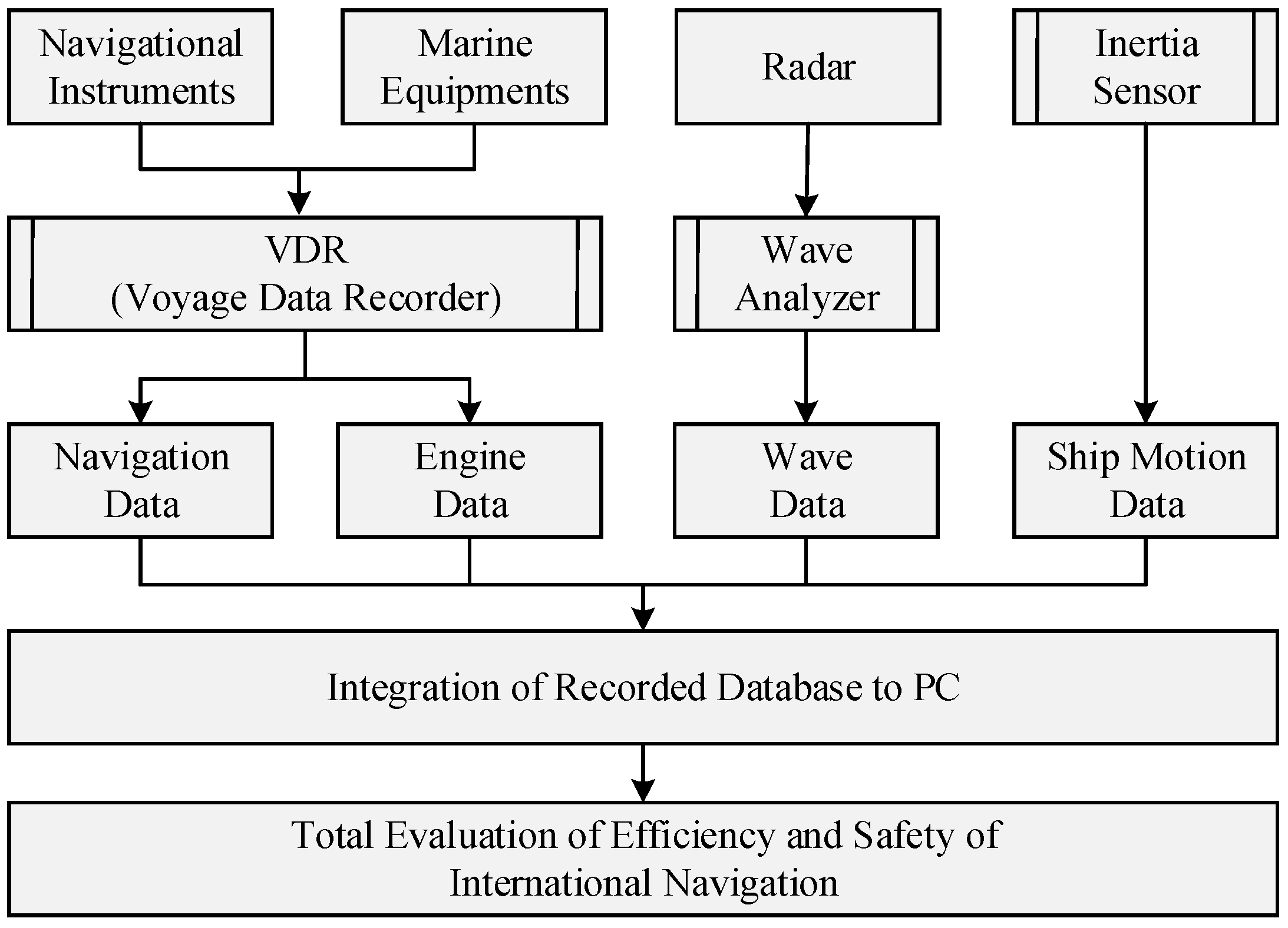
Data for this study were acquired through an integrated shipboard monitoring system, which incorporated a variety of sensors and instruments, as illustrated in Figure 1. The primary data acquisition systems included the following:

Global Positioning System (GPS): Continuously tracked the vessel’s location, speed over ground, and course, providing critical positional data for modeling ship movement and navigation.

Anemometer: Measured wind speed and direction, enabling the capture of atmospheric conditions that influence ship performance and fuel consumption.

Engine Monitoring System: Recorded key engine parameters, such as revolutions per minute (RPM), ship speed, and engine load, offering valuable insights into the vessel’s operational efficiency and power output.

Wave Radar: Measured wave height and direction, providing real-time data on sea state, which is essential for understanding the impact of environmental conditions on ship speed and stability.

Inertial Measurement Unit (IMU): Monitored the ship’s motion, capturing roll, pitch, and yaw, which are crucial for assessing the vessel’s dynamic behavior in response to environmental forces.

These systems collectively provided a comprehensive dataset that captured the ship’s operational and environmental conditions, essential for the predictive modeling of ship speed.

These instruments were connected to a central data logger, which recorded data at one-minute intervals. The high frequency of data recording allowed for the capture of transient phenomena, providing a detailed dataset for analysis.

2.2. Data Preprocessing

The multi-source energy data were continuously sampled over time, resulting in raw datasets that often-contained errors and anomalies due to factors such as ship docking, vessel swaying, data transmission delays, and other operational influences. For instance, while the normal range of engine speed typically falls between 100 and 200 RPM, the dataset contained anomalous readings, including engine speeds between 0 and 100 RPM. Similarly, for ship position, data samples with values of 0 or NaN were clearly erroneous and not representative of actual positions.

The preprocessing process began by removing obviously incorrect data points. Subsequently, abnormal values, including missing and outlier data, such as those that fall outside the physically reasonable range for ship navigation or environmental conditions (e.g., negative ship speeds, wave heights exceeding 50 m, wind speeds above 100 m/s), were addressed. Data samples with continuous gaps of 50 min or more were excluded, while missing values with durations shorter than 50 min were interpolated to fill the gaps.

The diversity of input features and differences in their dimensions can also adversely affect prediction results. Therefore, in this study, two types of collected data were normalized to support and enhance subsequent predictions. The principle of normalization is to control the values of different types of data within the same range, which can effectively eliminate the influence of feature scales on model performance and significantly improve the accuracy of predictions.

In this study, the Min-Max method was selected through comparative analysis for data normalization. This method maps all raw data to the [0,1] interval. The corresponding transformation formula is shown in Equation (1).

$${\overline{x}}_i={\displaystyle \frac{x_i-x_{\min }}{x_{\max }-x_{\min }}}$$

(1)

Environmental feature variables, such as wind speed and wind direction, have a significant impact on a ship’s energy consumption, and there are interactions among these factors. Numerous internal and external environmental factors related to the vessel can lead to considerable variations in energy consumption during navigation.

To improve the accuracy of the model, correlation analysis was conducted on the preprocessed data. Based on the results, the degree of correlation between different feature parameters can be determined, thereby providing support for subsequent analysis. Following these cleaning procedures, a final dataset comprising 10,226 valid data points was retained for ship speed prediction. A partial subset of the multi-source data after preprocessing is shown in

Table 1. Partial multi-source data after data processing.

Speed Over Ground (SOG) /(kn)	Wind Dir /(°)	Wind Speed /(m/s)	Engine Speed /(rpm)	Pitch Angle /(°)	Roll Angle /(°)	Wave Height /(m)	Wave Period /(s)	Wave Dir /(°)	Fuel Consumption /(Liter/Hour)
15.2	194	27.6	108	1.45	5.00	2.56	8.7	209	720
15.4	198	28.1	108	1.41	4.15	2.53	8.7	209	720
15.2	200	28.4	108	1.38	5.12	2.5	8.7	208	732
15.2	201	28.8	108	1.71	4.55	2.48	8.7	208	730
14.9	201	29.9	108	1.38	4.53	2.45	8.7	208	730
…	…	…	…	…	…	…	…	…	…

. The wind and wave direction are given in an absolute Earth-fixed reference system, with 0° corresponding to the north, increasing clockwise (i.e., 90° is east, 180° is south, etc.)

2.3. Correlation Analysis

It is important to recognize that various feature variables can influence real-time ship speed, and different characteristics may have differing levels of impact. Previous research has demonstrated the value of performing correlation analysis to identify key features that contribute to ship speed prediction while removing redundant or irrelevant variables. Ship speed is influenced not only by navigational state variables such as speed over ground (SOG), course over ground (COG), and engine speed, but also by environmental factors such as wind speed, wind direction, wave height, wave period, and wave direction.

In this study, Pearson’s correlation coefficient $r$ was employed to assess the relationships between the multi-source data variables. The formula for calculating r is shown in Equation (2), and the results of the correlation analysis, particularly the relationship between ship speed and various ship parameters, are presented in Figure 2.

$$r={\displaystyle \frac{{\displaystyle \sum _{i-1}^n\left(X_i-\overline{X}\right)\left(F_i-\overline{F}\right)}}{\sqrt{{\displaystyle \sum _{i-1}^n{\left(X_i-\overline{X}\right)}^2}}\sqrt{{\displaystyle \sum _{i-1}^n{\left(F_i-\overline{F}\right)}^2}}}}$$

(2)

where $X_i$ indicates the feature variables, $F_i$ indicates ship speed and represents its respective average values, and n represents the length of the variables. We then divide the correlation into 5 grades: very strong ($r$ > 0.65), strong (0.5 < $r$ < 0.65), moderate (0.35 < $r$ < 0.5), weak (0.2 < $r$ < 0.35), and very weak ($r$ < 0.2).

A detailed analysis of Figure 2 reveals the following insights: both wave height and wind speed show a negative correlation with ship speed. This indicates that under conditions of higher wind speeds and greater wave heights, the resistance to navigation increases, leading to a reduction in ship speed. In such scenarios, ship fuel consumption shows a positive correlation with wave height and wind speed. These results suggest that under harsh environmental conditions, fuel consumption increases, which negatively affects the vessel’s energy efficiency. Therefore, it is essential to fully account for this phenomenon during data processing.

Considering the interference caused by factors such as the ship’s navigation posture and meteorological conditions, internal variables were excluded in the modeling process. Ultimately, the selected feature variables include wind speed, wind direction, course, and wave height, which are used to predict the ship’s energy consumption and speed.

2.4. Models for Prediction

Model Selection

The selection of predictive models for this study was based on their ability to effectively handle nonlinear relationships and their demonstrated performance in previous research. The following models were chosen for their suitability to the problem at hand.

Backpropagation Neural Network (BPNN): Selected for its capability to model complex, nonlinear relationships between input variables. The BPNN is particularly effective for problems where the underlying relationships between data features are not explicitly known, making it ideal for capturing intricate patterns in the dataset. For the Backpropagation Neural Network (BPNN), we adopted a mini-batch training strategy with a batch size of 64, using 160 epochs. The Mean Squared Error (MSE) was selected as the loss function, and the ReLU activation function was used in the hidden layers. These settings were determined through grid search and training stability analysis.

Support Vector Regression (SVR): Chosen for its robustness in managing high-dimensional data and its ability to avoid overfitting, particularly in scenarios with smaller datasets. SVR is well suited for problems involving noisy or limited data. For the SVR model, we used the radial basis function (RBF) as the kernel. The penalty factor C was set to 10, and the gamma parameter was set to 0.23. These values were selected based on grid search optimization using 5-fold cross-validation.

Decision Tree (DT): Selected for its simplicity, interpretability, and ability to reveal hierarchical relationships among input features. DTs provide a transparent model, which is beneficial for understanding the decision-making process and identifying key contributing factors. For the Decision Tree (DT) model, we optimized key hyperparameters through grid search and cross-validation. The final configuration used in the experiments includes a maximum depth of 11, minimum samples split of 9, and a minimum sample of 1 per leaf. The max_features parameter was set to “auto”, allowing the model to automatically consider all input features during splits.

Random Forest (RF): An ensemble learning method that aggregates multiple Decision Trees to enhance prediction accuracy and robustness. RF excels in handling noisy datasets and missing data, offering improved generalization over individual Decision Trees. For the Random Forest (RF) model, we employed an ensemble of 150 Decision Trees. The hyperparameters were tuned using grid search and cross-validation. The optimal configuration included a maximum tree depth of 14, minimum samples required to split a node set to 8, and a minimum sample of 1 per leaf node.

XGBoost: An optimized and scalable implementation of the gradient boosting framework. It is widely recognized for its high performance, efficiency, and accuracy, especially in predictive modeling tasks involving structured/tabular data. For the XGBoost model, we set the number of boosting rounds to 140, with a maximum depth of 14 per tree. The learning rate was tuned to 0.09, and the minimum sample per leaf was set to 1. All hyperparameters were selected based on a combination of grid search and performance evaluation through cross-validation.

LightGBM: A high-performance, open-source gradient boosting framework developed by Microsoft. It is designed to be faster, more efficient, and more scalable than traditional gradient boosting algorithms like XGBoost, especially when dealing with large datasets and high-dimensional features. For the LightGBM model, the number of boosting iterations was set to 155, with a maximum depth of 13, and a learning rate of 0.076. The minimum sample per leaf was set to 1. These hyperparameters were selected based on grid search optimization to achieve the best trade-off between model accuracy and generalization.

2.5. Model Training and Validation

(1)

Data Splitting

The preprocessed dataset was partitioned into training and testing subsets using an 80–20 ratio. The training set, comprising 80% of the data, was utilized to develop and train the predictive models, while the remaining 20% of the data served as the testing set to evaluate model performance.

(2)

Cross-Validation

To assess the robustness and generalizability of the models, k-fold cross-validation was employed during the training phase. A 10-fold cross-validation approach was adopted, in which the dataset was randomly divided into ten subsets. For each iteration, one subset was used as the testing set, while the remaining nine subsets were used for training. This process was repeated ten times, with each subset serving as the testing set exactly once, ensuring a comprehensive evaluation of model performance across different data splits.

(3)

Model Optimization

Hyperparameter optimization was performed using grid search techniques to identify the best parameters for each model. For the Backpropagation Neural Network (BPNN), the optimization process focused on parameters such as the number of hidden layers, the number of neurons per layer, and the learning rate. In the case of Support Vector Regression (SVR), the kernel type (linear, polynomial, or radial basis function [RBF]) and regularization parameters were fine-tuned. For the Decision Tree (DT) and Random Forest (RF) models, the key hyperparameters optimized included tree depth, the minimum number of samples required to split an internal node, and the number of trees for the RF model. For XGBoost, a robust ensemble learning algorithm, several key hyperparameters were carefully tuned using grid search to enhance model generalization and control overfitting. And for LightGBM, a gradient boosting framework was optimized for efficiency and scalability.

2.6. Model Evaluation

The performance of each model was evaluated using the following metrics, as given in Equations (2)–(4):

• Mean Squared Error (MSE): Measures the average squared difference between predicted and actual values, providing a measure of the model’s accuracy.
• Root Mean Squared Error (RMSE): The square root of the MSE, providing a more interpretable metric by expressing the error in the same units as the output variable.
• R-Squared (R²): Indicates the proportion of the variance in the dependent variable that is predictable from the independent variables.

$$RMSE=\sqrt{{\displaystyle \frac{1}{m}}{\displaystyle \sum _{i=1}^m(y_i}-{\widehat{y}}_i{)}^2}$$

(3)

$$MAE={\displaystyle \frac{1}{m}}{\displaystyle \sum _{i=1}^m\left|(y_i-{\widehat{y}}_i)\right|}$$

(4)

$$R^2=1-{\displaystyle \frac{{\displaystyle \sum _i{({\widehat{y}}_i-y_i)}^2}}{{\displaystyle \sum _i{({\overline{y}}_i-y_i)}^2}}}$$

(5)

3. Results

3.1. Model Performance Comparison

To evaluate the predictive capability of each model, three standard performance metrics were employed: Root Mean Square Error (RMSE), Mean Absolute Error (MAE), and the coefficient of determination (R²). These metrics collectively assess both the accuracy and robustness of the models in ship speed prediction based on shipboard observational data. The performance comparison of all the models is summarized in

Table 2. Performance comparisons of all models.

	BP	SVR	DT	RF	XGBoost	LightGBM
RMSE	0.253	0.395	0.316	0.297	0.198	0.188
MAE	0.311	0.315	0.247	0.236	0.157	0.149
R2	0.951	0.850	0.930	0.934	0.973	0.978

.

3.2. Overall Model Performance

Among the models tested, LightGBM demonstrated the best overall performance, achieving the lowest RMSE (0.188) and MAE (0.149), alongside the highest R² score (0.978). This indicates a highly accurate and consistent prediction capability with minimal deviation from actual values.

XGBoost also performed exceptionally well, slightly trailing LightGBM with an RMSE of 0.198, MAE of 0.157, and R² of 0.973, showcasing its robustness in modeling nonlinear relationships and handling noisy, multivariate maritime data.

The Random Forest (RF) and Decision Tree (DT) models achieved reasonable accuracy, with RF slightly outperforming DT in all three metrics. The BPNN provided solid results, but its RMSE and MAE were notably higher than those of the boosting-based models.

In contrast, Support Vector Regression (SVR) yielded the lowest performance, particularly evident in its higher RMSE (0.395) and lower R² (0.850), suggesting limited capability in capturing the complex relationships present in the dataset.

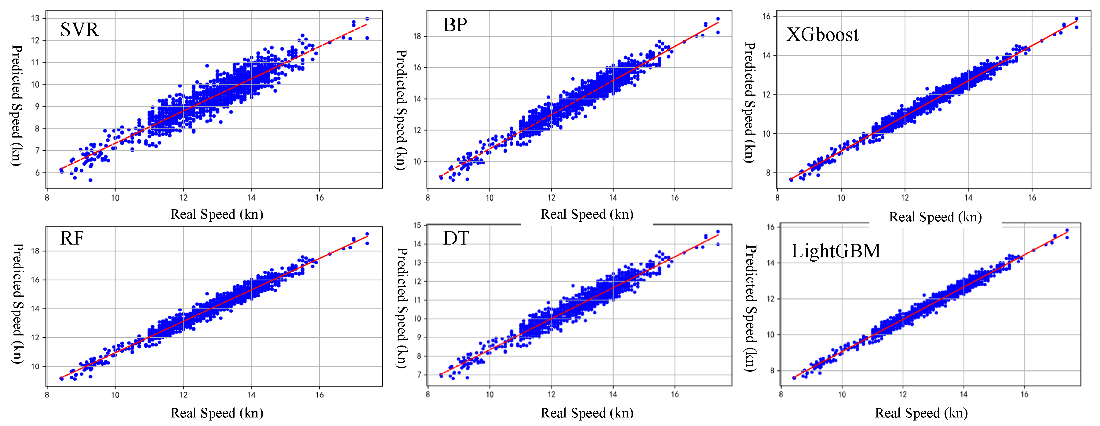
Overall, ensemble learning methods—particularly LightGBM and XGBoost—proved to be the most effective approaches for ship speed prediction in this study, offering strong generalization ability and prediction precision. To further illustrate the performance of the models, Figure 3 compares the predicted ship speeds against the actual ship speeds for all models, which were the top performers.

The plots reveal that the predictions from these models closely track the actual data, with only minor deviations. Among all the models, LightGBM exhibited the most accurate alignment with observed ship speeds across the entire range, demonstrating its strong ability to generalize and adapt to varying input conditions. The prediction points are densely clustered around the 45-degree reference line, indicating minimal error. Similarly, XGBoost produced highly reliable predictions, with slightly larger residuals in a few outlier cases, but it maintained a high degree of consistency overall.

The Random Forest (RF) and Decision Tree (DT) models also displayed good predictive capacity, though a slightly wider spread of data points around the reference line was observed, particularly at extreme values of ship speed. This suggests that while they can capture general trends, their performance may be slightly less stable under more variable conditions.

The Backpropagation Neural Network (BPNN) provided reasonably accurate predictions, but some under- and overestimations were observed, likely due to its sensitivity to the choice of network architecture and training parameters. In contrast, Support Vector Regression (SVR) showed the largest deviations, with less consistent tracking of actual speeds, reflecting its lower performance metrics.

In summary, the scatter plots in Figure 3 visually confirm the numerical evaluation results, reinforcing the conclusion that boosting-based ensemble models, particularly LightGBM and XGBoost, offer superior predictive accuracy and stability for ship speed prediction using shipboard observational data.

4. Discussion

4.1. Model Performance Analysis

The comparative analysis of multiple machine learning models—including the BPNN, SVR, DT, RF, XGBoost, and LightGBM—demonstrated that ensemble-based models, particularly LightGBM and XGBoost, consistently outperformed others across all evaluation metrics. LightGBM achieved the lowest RMSE (0.188) and MAE (0.149), along with the highest R² value (0.978), indicating its superior capability in learning complex, nonlinear relationships between ship operational and environmental parameters. XGBoost followed closely, also delivering highly reliable predictions.

The Random Forest and Decision Tree models, though less accurate than the boosting-based models, still achieved acceptable results, suggesting that tree-based architectures are well suited for ship speed prediction. The BPNN, despite its flexibility, showed moderate prediction accuracy, likely due to its sensitivity to hyperparameter tuning and potential to overfit on limited data. SVR performed the poorest among all models, struggling to capture the intricacies of the data distribution, especially under high environmental variability.

4.2. Factors Affecting Prediction Accuracy

Several factors were found to influence the prediction accuracy of the models:

(1)

Sensor-based shipboard observations often include noise, missing values, or asynchronous measurements. Models such as LightGBM and XGBoost are inherently robust to such imperfections due to built-in regularization and handling of missing data.

(2)

The inclusion of key environmental and operational variables—such as wind speed, wind direction, wave height, and course—was critical. These features have strong physical correlations with ship resistance and propulsion efficiency, directly affecting speed.

(3)

Ensemble models benefited from well-optimized hyperparameters and were less sensitive to overfitting compared to neural networks. On the other hand, simpler models like SVR suffered due to their limited capacity to handle nonlinearity and feature interaction.

(4)

The range and variability in the training data also impacted model generalization. LightGBM’s leaf-wise growth strategy allowed it to learn more specific patterns when sufficient diverse data were available.

4.3. Comparison with Existing Research

The findings of this study are consistent with the existing literature in the field of maritime machine learning applications. Previous research, such as that by Coraddu et al. [6], has also shown that ensemble methods outperform traditional regression and support vector-based approaches in ship performance prediction tasks.

Our results reinforce the trend observed in recent works toward the adoption of gradient boosting frameworks, which provide a balance between accuracy, interpretability, and computational efficiency. While earlier studies often focused on limited feature sets or simpler models, this study extends the analysis with a comprehensive dataset and detailed hyperparameter optimization across multiple model families.

4.4. Application Prospects and Limitations

The high predictive accuracy of boosting-based models like LightGBM suggests strong potential for real-world deployment in intelligent ship routing systems, performance monitoring platforms, and fuel efficiency optimization tools. These models can be embedded within decision-support systems for voyage planning, enabling more accurate speed forecasting under varying environmental conditions, and supporting strategies for emission reduction and energy savings. However, several limitations must be acknowledged:

(1)

The models were trained on data from a specific vessel or voyage pattern. Their performance on other ship types, routes, or climatic conditions may vary and require retraining or transfer learning.

(2)

Although feature importance metrics are available, models like LightGBM and XGBoost still function as “black boxes” to some extent, which may limit interpretability in critical decision-making scenarios.

(3)

While the models are computationally efficient during inference, real-time deployment requires integration with onboard systems and robust preprocessing pipelines to handle live sensor data and maintain data quality.

5. Conclusions

In this study, multiple machine learning models—including the Backpropagation Neural Network (BPNN), Support Vector Regression (SVR), Decision Tree (DT), Random Forest (RF), XGBoost, and LightGBM—were systematically evaluated for the task of ship speed prediction based on shipboard observational data. The following key conclusions can be drawn:

(1)

Among all models tested, LightGBM achieved the best overall performance, followed closely by XGBoost. Both models significantly outperformed traditional regression-based models and neural networks in terms of prediction accuracy, with LightGBM reaching an RMSE of 0.188 and an R² of 0.978.

(2)

Ensemble learning techniques, especially gradient boosting frameworks, demonstrated strong generalization ability and robustness to noisy and complex data. Their capability to model nonlinear relationships and handle high-dimensional features makes them well suited for maritime applications.

(3)

The application of high-performing machine learning models, particularly LightGBM and XGBoost, holds great promise for real-time decision support in ship routing, fuel consumption optimization, and emission reduction strategies. These models can serve as the foundation for intelligent maritime navigation and energy-efficient operations.

While the results are encouraging, the current models are trained on specific datasets, and their applicability to different ship types and routes requires further validation. Future research may focus on developing hybrid models that integrate physical and data-driven approaches, incorporating broader datasets, and enhancing model interpretability for operational deployment.