Abstract
The improved control performance of the buoy and winch collaborative control system can enhance the stability of the connection between underwater robots and ground industrial control equipment. To overcome the challenge of mathematical modeling of this control system, this research introduces reinforcement learning and transformer models in the design process. The main contributions include the development of two simulation environments for training DRL agents, designing a reward function to guide the exploration process, proposing a buoy control algorithm based on the discrete soft actor-critic (SAC) algorithm, and proposing a winch cable length prediction algorithm based on a lightweight transformer model. The experiment results demonstrated significant improvements in rewards diagrams, buoy control trajectories, and winch model performance, showcasing the effectiveness of our proposed system. The average error of the buoy tracking trajectories induced by different policies trained in the two environments is less than 0.05, and the evaluation error of the behavior cloning lightweight transformer model is less than 0.03.
1. Introduction
The integration of artificial intelligence technology into underwater robots has paved the way for the implementation of underwater tasks, including territorial sea exploration and monitoring of underwater facilities. However, advanced underwater robots face hardware limitations and necessitate a host computer to supply computing resources. They also require real-time positioning on the water surface to prevent economic losses resulting from signal loss. Consequently, underwater robots frequently need to establish a connection with the host computer and control unit via cables to achieve stable real-time scheduling. The data generated from the buoy play a crucial role in devising observation policies and analyzing the motion status of underwater robots [1]. Moreover, a collaborative control system, consisting of a winch and a buoy, is employed to regulate the cable length and prevent it from breaking due to entanglement by external forces. Thus, a pivotal challenge for underwater robots is to enhance the control performance of the buoy and winch collaborative control system, ensuring that it aligns with the pertinent requirements for underwater robot operations.
The buoy and winch control system can help underwater vehicles operate stably in complex waters and improve the efficiency and safety of operations [2]. Liu et al. [3] introduced a data collection scheme designed for unmanned aerial vehicle (UAV)-assisted ocean monitoring networks (OMNs), aiming to optimize the energy efficiency of the IoUT. Shin et al. [4] proposed an optimization method that combines the beam divergence angle and transmission power level in an underwater sensor to maintain optical beam alignment in underwater optical wireless communication (UOWC) for buoys. Meanwhile, a lot of control technologies have been proposed to improve the control effect of buoys and winches. Wei et al. [5] used the fuzzy PID self-tuning control method and IIR digital filter to reduce the interference of sea waves during the data collection process, and proposed a data acquisition control system with automatic lifting for buoy control. Liu et al. [6] proposed a model-free buoy control scheme with a robust exact differentiator that outperforms the root mean square error of conventional proportion differentiation controllers. Vallegra et al. [7] designed an efficient collective operation of heterogeneous systems consisting of 22 autonomous buoys. Zhang [8] proposed a multiple buoy control platform based on BeiDou difference, with in-field recording tests at Tianjin port verifying the effectiveness of the control system. To solve the problem of dynamic optimization of ping schedules in an active sonar buoy network, Saksena et al. [9] proposed a novel ping optimization method, based on the application of approximate partially observable Markov decision process (POMDP) techniques, which can also be regarded as the first method that applied reinforcement learning (RL) to a buoy control system. Sarkisov et al. [10] proposed a winch-based actuation method for crane-stationed cable-suspended aerial manipulators. With a winch control system, aerial manipulation systems achieve the ability to generate a wrench that reduces the effect of gravitational torque. Kim et al. [11] proposed a winch device that allows a tether to spool or unspool underwater to adjust the tether length of underwater robots. Generally, these methods require precise and well-designed mathematical models. However, it is difficult to obtain an explicit mathematical model of a real environment due to many contingencies. Therefore, we consider introducing deep reinforcement learning algorithms (DRL) into buoy and winch control systems.
With the rapid development of artificial intelligence, many advanced algorithms have been introduced into robotic control tasks. In recent years, there has been a notable surge, particularly in the utilization of transformer models and reinforcement learning techniques for robotic control tasks. Staroverov et al. [12] proposed multimodal transformer models, which can process and integrate information from multiple modalities, such as vision, language, and sensory inputs, to generate actions in various environments. Meanwhile, Liu et al. [13] presented a robotic continuous grasping system that employs a shape transformer to estimate the position of multiple objects simultaneously. Núñez et al. [14] focused on the application of transformer and multi-layer perceptron (MLP) models for classification in an anthropomorphic robotic hand prosthesis using myoelectric signals. Masmitja et al. [15] investigated the use of reinforcement learning for the dynamic tracking of underwater targets by robots. This study explores the challenges and opportunities of applying long short-term memory (LSTM) and soft actor-critic(SAC) algorithms to AUV controlling tasks, with a focus on improving tracking accuracy and robustness. Hu et al. [16] proposed a trajectory tracking control system for robotic manipulators that combines SAC and ensemble random network distillation, which improves the precision and adaptability of robotic manipulators in complex tasks. Additionally, Dao and Phung [17] proposed a robust integral of sign of error (RISE)-based actor-critic reinforcement learning control method for a perturbed three-wheeled mobile robot with mecanum wheels. The method introduced a nonlinear RISE feedback term-associated discount factor to eliminate dynamic uncertainties from an affine nominal system. On the other hand, Han et al. [18] proposed an actor-critic reinforcement learning framework for controlling 3D robots, incorporating a Lyapunov critic function to guarantee closed-loop stability.Furthermore, the combined offline reinforcement method decision transformer using a transformer model achieved better control performance in many control tasks [19]. Collectively, these studies underscore the immense potential of transformer models and reinforcement learning techniques in enhancing the capabilities of robots across various environments. By harnessing these advanced machine learning methodologies, researchers have significantly improved the performance, accuracy, and adaptability of robotic systems in control tasks and trajectory tracking.
Inspired by those AI control works, we consider using reinforcement learning and a transformer model to achieve collaborative control between the buoy and winch. Thus, we decomposed the collaborative control system into a buoy control system based on a DRL algorithm and a winch control system based on a behavior cloning transformer model.
The main contributions of this research include the following: (a) Development of a simulation environment for training DRL agents using a multi-agent particle environment (MPE). (b) Designing a reward function with a bonus to guide the exploration process of agents in the environment. (c) Proposing a buoy control algorithm based on the discrete SAC algorithm. (d) Proposing a winch cable length prediction algorithm based on a lightweight transformer model.
Subsequent experimental analyses were conducted for the following: (a) Analyzing the impact of reward bonuses on buoy control performance under various parameters and different environmental settings. (b) Analyzing the training effects of different reward components under diverse environmental settings. (c) Demonstrating the buoy control effect and validating the effectiveness of the SAC-based buoy control algorithm. (d) Collecting offline experience data through the trained buoy control system and presenting the training effect of the lightweight transformer, thus confirming the algorithm’s effectiveness.
2. Related Work
DRL, a fusion of deep learning and RL, serves as an algorithmic solution for complex decision-making problems. Some popular DRL algorithms are popular in control applications. DeepMind proposed the proximal policy optimization (PPO) method [20], widely used for training RL agents in diverse applications. Afterwards, Fujimoto et al. [21] combined the double DQN and DDPG method, introducing the twin delayed deep deterministic policy gradient (TD3) method. Subsequently, investigating the equivalence between policy gradient and value iteration [22], Haarnoja [23] proposed the soft actor-critic (SAC) method. The inclusion of maximum entropy regularization in SAC proves advantageous in encouraging exploration during the learning process. This algorithm proves particularly effective when dealing with situations where the specific mathematical model is unknown, allowing the agent to generate superior policies through environment exploration [24].
With the rapid development of RL algorithm applications, many RL methods have been used in buoy or other underwater vehicle control tasks. Zhang et al. [25] introduced the reinforcement learning method into the buoy control system to maximize the operational duration of smart buoys while ensuring normal power consumption for each sensor. Hribar et al. [26] designed a deep deterministic policy gradient which can significantly extend the sensors’ lifetime. Su et al. [27] proposed a DRL-based latching duration strategy to amplify a wave energy converter’s (WEC) response to wave motion. Zheng et al. [28] proposed a novel end-to-end multi-sensor fusion algorithm rooted in DRL to maximize the efficiency of underwater acoustic sensor networks (UASNs). Hu et al. [29] proposed two on-policy hierarchical actor-critic algorithms which reduce the economy, security, and fairness costs of grid control. Sivaraj [30] proposed a set of continuous state-action space-based DRL algorithms to generate path following of a ship in calm water and waves. Kouzehgar et al. [31] proposed a modified version of the multi-agent deep deterministic policy gradient (MADDPG) approach and a reward function that intrinsically leads to collective behavior. Recently, several DRL algorithms have been applied to the design of buoy and winch control systems. Bruzzone et al. [32] proposed a simple and low-cost RL-based wave energy converter to dynamically adjust the generator speed–torque ratio as a function of the sea state, which can efficiently decrease the motion of buoys caused by the waves. Liu et al. [33] proposed an RL-based obstacle avoidance controller for the path planning task of a robot with a fixed-length cable connected to a mobile base. Experimental results prove that the RL algorithm can help cables dynamically avoid obstacles. Liang et al. [34] designed a multi-agent DRL algorithm based on a hybrid discrete and continuous action space to generate the transmission power of buoys. The DRL-based buoy control system learns a criteria and higher spreading of agents for area coverage. Among these studies, there is a lack of application of DRL in the domain of buoy and winch collaborative control systems.
3. Training Environment
3.1. Buoy and Winch Control Environment
Based on MPE, we build an RL environment to simulate the underwater robot, buoy, and winch control scenarios. The environment is shown in Figure 1, including three dots and three perspectives. Among them, three dots with different colors are marked, respectively:
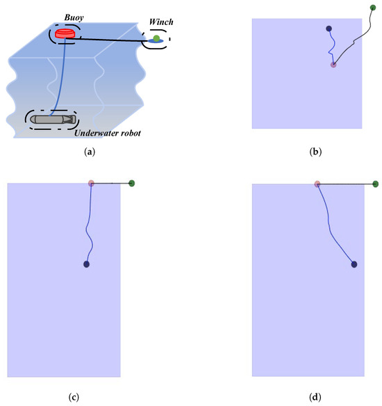
Figure 1.
Diagrams of the environment: (a) schematic diagram of the work scenario; (b) main view of the environment; (c) top view of the environment; (d) left view of the environment.
(a) The green dot represents the winch. Generally, when the underwater robot is working, the winch must be fixed on the shore, so the green dot will remain stationary and will not shift after initialization.
(b) The pink dot represents the buoy, serving as a controllable agent in the environment. The objectives for training this agent are as follows: 1. Keep the underwater umbilical cable vertical to prevent the cable from wrapping around itself or becoming entangled with the underwater robot. 2. The buoy should only move horizontally on the water surface and remains relatively stationary with the underwater robot in the horizontal direction.
(c) The black dot represents the underwater robot operating underwater and can move horizontally and vertically; it is responsible for underwater detection.
(d) The blue box in the picture is the movable water area, and underwater robots and buoys will only operate within this range.
The observation and action space of the environment are defined as follows:
(a) The state s of the environment includes the following parts: the buoy coordinates , the underwater robot coordinates , the relative distance , the buoy speed vector , the underwater robot speed vector , buoy speed, and the buoy angular velocity .
(b) The dynamic buoy uses discrete movements to control the horizontal displacement direction, including north, south, west, east. When the action is 0, the buoy is stationary; when the action is 1, the buoy runs north; when the action is 2, the buoy runs south; when the action is 3, the buoy runs east; and when the action is 4, the buoy runs west.
3.2. Cable Simulation
Set the dots which represent the positions of the winch, buoy, and underwater robot to A, B, and C. Then, the cable in the environment will be divided into two parts: the surface cable and the underwater cable . Furthermore, in order to reduce the computational complexity of the cable simulation, the underwater cable is decomposed into a horizontal cable and a vertical cable . Therefore, the environment contains three cables: , , and , and the corresponding number of cable nodes are , , and .
(a) As shown in Figure 2a, the black line segment AB represents cable . The cable end is connected to the winch, and the cable head end is connected to the buoy. Winch point A is fixed, so the cable end remains stationary, while the cable head end tracks the buoy’s movement. On the other hand, the buoy does not dive or float, allowing the line segment to directly simulate the stretching and deformation of the umbilical cable in the water.
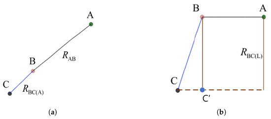
Figure 2.
Diagrams of the cables: (a) top view of the simulated ropes; (b) main view of the simulated ropes.
(b) As shown in Figure 2a, the blue line segment BC represents cable . The cable end is connected to the buoy, and the cable head is connected to the underwater robot. In the environment, the points on the line segment BC are only affected by the horizontal force from the buoy and the underwater robot.
(c) As shown in Figure 2b, the brown line segment BC’ represents the vertical projection of cable . In the environment, the points on the line segment BC’ are only affected by the vertical force from the buoy, the underwater robot, and gravity.
3.3. Reward Function
On the one hand, DRL algorithms with low sample efficiency require special reward functions to guide agent training [35]. The buoy needs to move to the target location quickly, and a sparse reward function will increase the difficulty for the agent to find the target. Therefore, we set a basic reward function that is positively related to the buoy tracking effect.
3.3.1. Basic Reward
The definition of basic reward is designed as follows:
The idea is that as the horizontal distance between the buoy and the underwater robot increases, the reward value rises. Conversely, when this distance decreases, the base reward value decreases. By providing continuous base rewards, we can motivate the agent to reduce the horizontal gap between the buoy and the robot. Essentially, offers a straightforward way to gauge how well the buoy is being tracked. However, relying solely on as a training criterion still has its drawbacks.
3.3.2. Bonus Reward
When the buoy is far away from the target position, will be a small negative value. However, when the buoy is close to the target position, will tend to 0, and the change amplitude of the state value will also tend to 0. Thus, the agent is not able to receive equivalent positive encouragement for the behavior of staying at the target location, which is much smaller than the reward for moving to the target location. Therefore, we design the bonus reward to guide the agent to stay within a very close distance of the target point.
The idea is that as the buoy maintains a horizontal distance of less than 0.05 from the underwater robot, an incremental bonus reward will be given to accelerate the learning of the agent. On the other hand, once the buoy deviates from the underwater robot by more than 0.05, the bonus will be cleared. Thus guides the agent to stay close to the underwater robot for a long time.
3.3.3. Rope Reward
In terms of safety performance, in actual application scenarios, excessive vibration of the umbilical cable will increase the probability that the cable will become entangled with itself or become entangled with the equipment. Thus, we design the rope reward:
Its physical meaning is as follows: a reward negatively related to the length of the cables and , used to reduce the umbilical cable jitter caused by the RL policy.
Ultimately, the final reward function is as follows:
4. Control Algorithm
First of all, in actual scenarios, there are complex environmental noises such as obstacles and water flow speeds in the dam. This type of highly random noise is difficult to express through traditional control algorithms. On the other hand, the buoy-winch coordinated control system has two controlled objects: the buoy and the winch. The control equations of the two control objects are highly coupled. Changes in the buoy’s movement direction and movement speed have different ideal umbilical cable lengths. If the winch does not release the umbilical cable length that meets the needs of the current scenario, there is a high probability that the cable will become entangled or broken. Therefore, collaborative control systems are difficult to model.
This article divides the buoy-winch coordination control system into two parts: the buoy control system and the winch control system. The two systems are implemented using machine learning algorithms that meet the system characteristics. The control logic of the two control systems are as follows: (1) a SAC-based buoy control algorithm; (2) a lightweight transformer-based winch control algorithm.
4.1. SAC-Based Buoy Control Algorithm
Since the state-action space is relatively complex, DRL algorithms are considered to optimize the control policy of the buoy. Usually, the acquisition of new knowledge relies on online exploration. However, random exploration will introduce new variance and increase the instability of policies, resulting in lower sample efficiency of the RL algorithm [36].
The reward function and learning target components in the environment are relatively complex, so the buoy control system requires a more efficient exploration algorithm. The DRL algorithm based on maximizing policy entropy can effectively improve the sample efficiency and policy stability of the algorithm. Thus, the discrete SAC algorithm [37] is used to implement the buoy control system.
Assume the dimension m of the action space, the action vector is . The value function iteration function is as follows:
where represents the transpose of vector x, the policy vector of discrete action is , is the temperature parameter which determines the relative importance of the entropy term versus the reward, and the Q value vector is . The update objection of the Q value net is
where represents the target value function, gives the distribution over the next state given the current state and action, and each transition is sampled from the experience replay buffer D. The soft expectation value is calculated over the state-action distribution.
The update objection of the temperature parameter is
where is a constant vector equal to the hyperparameter representing the target entropy.
Finally, the update objection of the actor network is as follows:
where represents the Q value vector induced by the Q value net .
4.2. Lightweight Transformer-Based Winch Control Algorithm
The length of the cable output by the winch will directly determine the safety performance of the control system: if the cable released by the winch is too long, although it will not bring additional pulling force to the underwater robot, it will increase the risk of cable entanglement; if the cable released by the winch is too short, it will apply extra tension to the cable, increasing the risk of the umbilical cord being torn. Therefore, this study opts for a deterministic algorithm to estimate the expected cable length for the movement of the underwater robot and buoy.
The control system primarily employs the behavior cloning algorithm, which directly learns the mapping of states to expert actions through a function approximation method. The input state is defined as the environmental information collected by the winch from the Ethernet, and the output action is the length of the three cables: , , and . The expert action corresponds to the experience data induced by the trained buoy control policy. In place of the traditional function approximation method, a lightweight transformer model with enhanced learning efficiency is adopted for behavior cloning to efficiently learn environmental information.
As showed in Figure 3, the lightweight transformer model only contains a multi-head attention module [38]. Following the encoding of the sequence by the embedding layer, positional encoding based on time steps is introduced. The data are then fed into the multi-head attention layer, followed by the feedforward neural network. After passing through the normalization layer and fully connected layer, the model outputs the expected cable length.
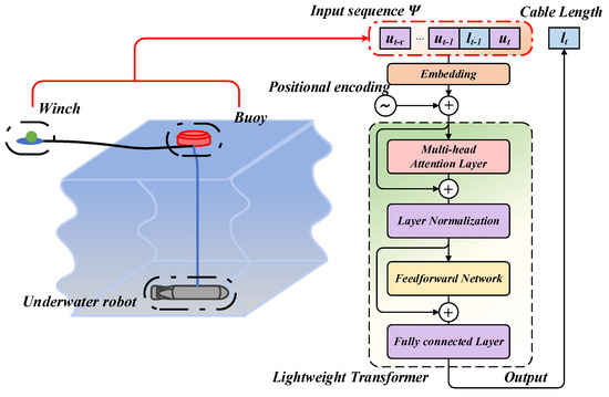
Figure 3.
Diagram of the lightweight transformer based winch control algorithm.
The input sequence is a set of environmental information from the previous steps. Every time step, the transition provided by the environment is . Where the state , represents the depth of underwater robot. , which is the vector of the lenth of surface cable and underwater cables and .
The update objection of the lightweight transformer model can be concluded as the following formula:
where q is the input sequence of the lightweight transformer and , and B is the offline experience buffer.
Based on the offline experience buffer B of the environment, the lightweight transformer, employing the behavioral cloning method, can dynamically forecast the anticipated length of the current cable in real time. Thus, the winch adjusts the umbilical cable length based on the real-time behavior of the underwater robot and buoy. This adaptive control mechanism helps prevent entanglement or breakage, facilitating the collaborative control of the winch and buoy.
5. Experiment Result
5.1. Buoy Control System
5.1.1. Environment Settings
If the underwater robot exhibits random behavior, it could lead to difficulties in the buoy tracking process, exacerbating the limitations stemming from the low sample efficiency inherent in DRL algorithms. Conversely, if the underwater robot remains stationary, the agent will not gather adequate environmental information. To address this, we devised two distinct environments, denoted as and , each configured with unique settings. This allows us to assess how different environments and reward structures influence the learned policy of the buoy control system.
(a) : Environment with stationary underwater robot
In , both the underwater robot and buoy start with randomly initialized coordinates. Throughout the episode, the underwater robot remains stationary, while the buoy, acting as the controlled entity, has the freedom to move. The optimal policy in this scenario is to efficiently guide the buoy to the target coordinates.
(b) : Environment with random walking underwater robot
shares the same initialization as . During the episode, both the underwater robot and buoy have the freedom to move. The agent takes on the role of the buoy, and the optimal control policy involves directing the movement of the buoy to overlap with the underwater robot at each time step.
The algorithm proposed in this article undergoes training in both environments. The trained policy is tested in both the training and evaluation phases. During training, the agent selects actions based on the probability distribution generated by the actor network. In the evaluation phase, the agent acts greedily, choosing the action with the highest probability. For ease of subsequent experimental analysis, we denote the policy obtained by training the agent in environment as . Additionally, the settings of hardware, software, and some hyper parameters are shown in Table 1 and Table 2.

Table 1.
Hardware and operating system specifications.
Table 2.
Software configuration and training parameters for SAC.
5.1.2. Bonus Reward Settings
In this section, we delve into the impact of the parameter in bonus rewards on the training of DRL, employing surface graphs and surface projections to analyze . The parameter is systematically varied across values of 1, 2, 3, and 5, and the agent undergoes training in both and . Contrasting with the final reward r, the basic reward provides a more intuitive reflection of the buoy’s tracking performance. Consequently, we present surface graphs and surface projections that capture the changing trend of . The specific experimental diagram is outlined below.
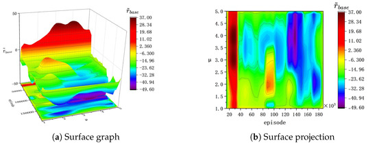
Figure 4.
of the training process in .
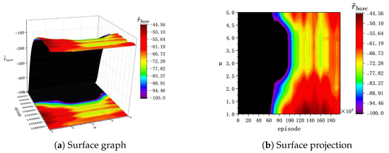
Figure 5.
of the evaluation process in .
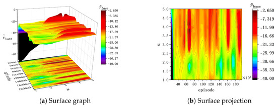
Figure 6.
of the training process in .
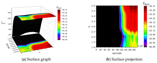
Figure 7.
of the evaluation process in .
(a) In , before the 40k episode during the training process, bonus rewards effectively enhance the speed of policy optimization. However, after 40k episodes and with , a noticeable degradation trend is observed in during training. This suggests that the agent no longer performs policy optimization and falls into a local optimum. Therefore, a larger value in bonus rewards increases the likelihood of overfitting in agent training within .
(b) In , both during training and evaluation, higher values of correspond to a higher achieved by the agent, with displaying a more pronounced upward trend. Consequently, in the context of , a higher effectively improves the buoy’s tracking performance. Therefore, under the setting of , a higher effectively improves the buoy’s tracking performance.
(c) In , during the evaluation process, there is a negative correlation between the buoy’s tracking effectiveness and the parameter . In contrast, in , during the evaluation process, there is a positive correlation between the changing trends in the basic reward and the parameter .
5.1.3. Reward Content Analysis
Based on the analysis in (1) of bonus reward settings, we take the agents of in and in as two typical cases to analyze the reward components. There are differences in the magnitude of rewards under different environments, so we normalize all rewards to the interval [0,1] and draw reward curves to analyze the components of reward functions in two types of environments.
As shown in Figure 8, the underwater robot remains stationary in , enabling the agent to easily accrue bonus rewards. Therefore, during the training process, the final reward r is dominated by bonus reward . This elucidates the observed policy degradation phenomenon in the training process within ; the bonus reward function is designed by logic and is not continous, and its variance is positively correlated with . Thus, higher leads to higher variance, which results in the non-monotonic policy optimization. In contrast, during training in , where the underwater robot moves randomly and the bonus reward remains elusive in the long term, the final reward r is governed by the basic reward with minimal variance. Moreover, larger values grant the agent additional rewards for tracking behaviors.
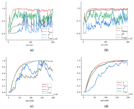
Figure 8.
Diagrams of rewards: (a) training process reward components in ; (b) training process reward components in ; (c) evaluation process reward components in ; (d) evaluation process reward components in .
On the other hand, the reward component curves of the evaluation process reveal that, despite the pronounced jitter in the and curves in , the evaluation policies and undergo monotonic optimization.
Afterwards, in order to further analyze the reward components, we provide interval diagrams of , , and in Figure 9, Figure 10 and Figure 11. In the legends of the interval diagrams, represents the statistical interval corresponding to the entire set of reward data obtained by the agent in , where specifically refers to the statistical interval corresponding to the last 10% of the reward data acquired in . The ensuing conclusions are as follows:
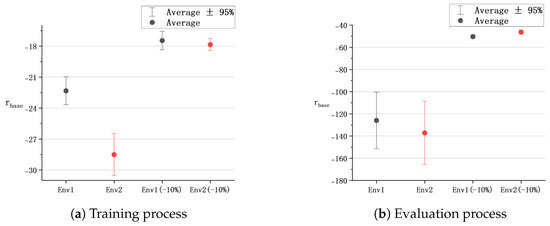
Figure 9.
Interval diagrams of .
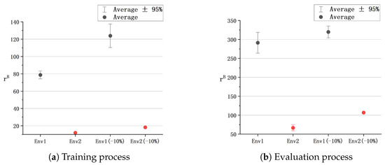
Figure 10.
Interval diagrams of .
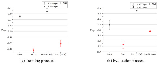
Figure 11.
Interval diagrams of .
(a) According to the interval diagram of the basic reward , it can be seen that in the early stage of training, the tracking effect of the agent trained in is better than that in . However, as experience data accumulate, agents in exhibit overfitting issues, leading to the degradation of policy . The experiment results corroborate that remains relatively stable and exhibits superior tracking performance.
(b) According to the interval diagram of the bonus reward , in both training and evaluation processes, the variance in the bonus reward obtained in significantly exceeds that in . Such high reward variance poses an impediment to the training of deep learning algorithms.
(c) It is noteworthy that the value of the rope reward correlates positively with the buoy’s jitter frequency. The interval diagram for illustrates that, in both training and evaluation processes, the values and variances obtained by the trained agent in outperform those in . That is, compared to , effectively mitigates cable shaking and demonstrates superior safety performance.
In summary, since the target position in remains unchanged, is more accustomed to conservative displacement and reduces the jitter of the cable. In , where the target position changes at each time step, adeptly tracks underwater robots with complex behavior.
5.1.4. Buoy Control Effect
We manually designed two trajectories: tractory , where the target position changes frequently; and tractory , where the target position changes slowly. The tracking effects of and are tested, respectively. The specific control trajectory diagram is shown in Figure 12 and Figure 13.
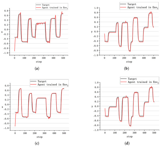
Figure 12.
The tracking effect of : (a) trajectory projection of x-axis induced by ; (b) trajectory projection of y-axis induced by ; (c) trajectory projection of x-axis induced by ; (d) trajectory projection of y-axis induced by .
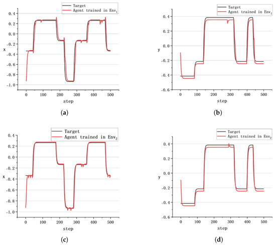
Figure 13.
The tracking effect of : (a) trajectory projection of x-axis induced by ; (b) trajectory projection of y-axis induced by ; (c) trajectory projection of x-axis induced by ; (d) trajectory projection of y-axis induced by .
Therefore, the following perspectives can be discerned:
(a) mainly provides experience data of the buoy moving to a stationary target position. Consequently, the efficacy of during the initialization phase surpasses that of due to specialized training within .
(b) The more frequently the target position changes, the worse the control effect of is. This is attributable to being inadequate in supplying sufficient environmental information to the agent, resulting in a challenge for to adeptly respond to rapid alterations in the target position.
(c) exhibits superior tracking capabilities, evidenced by significantly reduced trajectory jitter compared to .
In general, the buoy control algorithm based on SAC demonstrates a heightened response speed. Nonetheless, a certain degree of control signal error persists, necessitating additional filtering and stabilizers to enhance the ultimate control effectiveness.
5.2. Winch Control System
Initially, we gather offline experiential data from and to form behavior clone datasets, employing the trained policy . The behavior clone dataset comprises a total of 160k transitions, derived from 80 episodes in each environment, where each episode spans 100 sampling time steps. Subsequently, we embark on training a lightweight transformer model using this behavior clone dataset. The parameters of the lightweight transformer is shown in Table 3.
Table 3.
Training parameters for lightweight transformer.
For the transformer model used in the training process, the sequence length is set to 50, the attention heads are set to 7, and the hidden layer of the feedforward neural network contains 100 neurons. The specific loss convergence situation is shown in Figure 14.
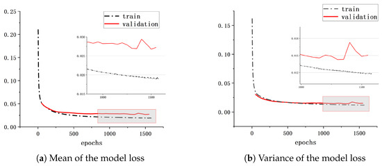
Figure 14.
The training effect of lightweight transformer.
As shown in Figure 14, the average evaluation error is below 0.03, and the training error is beneath 0.02. Furthermore, the evaluation error variance is less than 0.018, while the training error variance is below 0.015. This indicates that the lightweight transformer model adeptly captures the implicit relationship between environmental information and cable length, acquired from the behavior clone dataset. Moreover, it demonstrates high accuracy in predicting cable length in unfamiliar paths. Consequently, we posit that the lightweight transformer model can proficiently forecast cable lengths through behavioral cloning methodologies.
6. Conclusions
In this paper, we have presented a reinforcement learning (RL) approach for collaborative control between buoys and winches in underwater operations. We have introduced model-free algorithms based on soft actor-critic (SAC) and lightweight transformers, which enable efficient and adaptive control strategies. Through experimental evaluations, we have demonstrated that our proposed approach achieves a significant reduction in response time and an overall enhancement in controller performance compared to traditional methods. Our results highlight the potential of RL for underwater robotic operations, offering a promising direction for future research. However, we also acknowledge some limitations in our current approach, particularly in terms of control curve jitter, which may be addressed by exploring continuous action spaces and incorporating filters or alternative control methods.
To further refine our proposed approach, future research should focus on evaluating its robustness across diverse underwater conditions, such as varying currents and depths. Additionally, it would be beneficial to investigate the adaptability of our methods to different models and configurations of underwater robotic systems. Overall, our work paves the way for more advanced and intelligent underwater robotic operations, with the potential to revolutionize marine exploration and resource extraction.
Author Contributions
Software, Y.G.; Data curation, H.Y.; Writing—original draft, Y.G.; Writing—review & editing, J.N., Z.G. and B.Z.; Funding acquisition, J.N. All authors have read and agreed to the published version of the manuscript.
Funding
This research was funded by national key R&D program of china, grant number 2022YFB4703402.
Institutional Review Board Statement
Not applicable.
Informed Consent Statement
Not applicable.
Data Availability Statement
Publicly available datasets (including the environment and lightweight transformer model) were analyzed in this study. This data can be found here: https://github.com/sweetpot-to/Buoy-and-Winch-Collaborative-Control-System-Based-on-Deep-Reinforcement-Learning, accessed on 5 February 2025.
Conflicts of Interest
Author Zaiming Geng was employed by the company China Yangtze Power Co., Ltd. The remaining authors declare that the research was conducted in the absence of any commercial or financial relationships that could be construed as a potential conflict of interest.
References
- Cai, W.; Liu, Z.; Zhang, M.; Wang, C. Cooperative artificial intelligence for underwater robotic swarm. Robot. Auton. Syst. 2023, 164, 104410. [Google Scholar] [CrossRef]
- Viel, C. Self-management of ROV umbilical using sliding element: A general 3D-model. Appl. Ocean Res. 2024, 151, 104164. [Google Scholar] [CrossRef]
- Liu, Z.; Meng, X.; Yang, Y.; Ma, K.; Guan, X. Energy-Efficient UAV-Aided Ocean Monitoring Networks: Joint Resource Allocation and Trajectory Design. IEEE Internet Things J. 2022, 9, 17871–17884. [Google Scholar] [CrossRef]
- Shin, H.; Kim, S.M.; Song, Y. Learning-aided Joint Beam Divergence Angle and Power Optimization for Seamless and Energy-efficient Underwater Optical Communication. IEEE Internet Things J. 2023, 10, 22726–22739. [Google Scholar] [CrossRef]
- Wei, Y.; Wu, Y.; Zhang, X.; Ren, J.; An, D. Fuzzy self-tuning pid-based intelligent control of an anti-wave buoy data acquisition control system. IEEE Access 2019, 7, 166157–166164. [Google Scholar] [CrossRef]
- Liu, Q.; Li, M. Tracking control based on gps intelligent buoy system for an autonomous underwater vehicles under measurement noise and measurement delay. Int. J. Comput. Intell. Syst. 2023, 16, 36. [Google Scholar] [CrossRef]
- Vallegra, F.; Mateo, D.; Tokić, G.; Bouffanais, R.; Yue, D.K.P. Gradual collective upgrade of a swarm of autonomous buoys for dynamic ocean monitoring. In Proceedings of the OCEANS 2018 MTS/IEEE Charleston, Charleston, SC, USA, 22–25 October 2018; pp. 1–7. [Google Scholar]
- Zhang, H.; Zhang, D.; Zhang, A. An innovative multifunctional buoy design for monitoring continuous environmental dynamics at tianjin port. IEEE Access 2020, 8, 171820–171833. [Google Scholar] [CrossRef]
- Saksena, A.; Wang, I.J. Dynamic ping optimization for surveillance in multistatic sonar buoy networks with energy constraints. In Proceedings of the 2008 47th IEEE Conference on Decision and Control, Cancun, Mexico, 9–11 December 2008; pp. 1109–1114. [Google Scholar]
- Sarkisov, Y.S.; Coelho, A.; Santos, M.G.; Kim, M.J.; Tsetserukou, D.; Ott, C.; Kondak, K. Hierarchical whole-body control of the cable-suspended aerial manipulator endowed with winch-based actuation. In Proceedings of the 2023 IEEE International Conference on Robotics and Automation (ICRA), London, UK, 29 May–2 June 2023; pp. 5366–5372. [Google Scholar]
- Kim, J.; Kim, T.; Song, S.; Yu, S.C. Parent-child underwater robot-based manipulation system for underwater structure maintenance. Control Eng. Pract. 2023, 134, 105459. [Google Scholar] [CrossRef]
- Staroverov, A.; Gorodetsky, A.; Krishtopik, A.; Izmesteva, U.; Yudin, D.; Kovalev, A.; Panov, A. Fine-tuning multimodal transformer models for generating actions in virtual and real environments. IEEE Access 2023, 11, 130548–130559. [Google Scholar] [CrossRef]
- Liu, J.; Sun, W.; Liu, C.; Zhang, X.; Fu, Q. Robotic continuous grasping system by shape transformer-Guided multiobject category-Level 6-D pose estimation. IEEE Trans. Ind. Inform. 2023, 19, 11171–11181. [Google Scholar] [CrossRef]
- Montoya, B.N.; Añazco, E.V.; Guerrero, S.; Valarezo-Añazco, M.; Espin-Ramos, D.; Farfán, C.J. Myo transformer signal classification for an anthropomorphic robotic hand. Prosthesis 2023, 5, 1287–1300. [Google Scholar] [CrossRef]
- Masmitja, I.; Martín, M.; O’Reilly, T.; Kieft, B.; Palomeras, N.; Navarro, J.; Katija, K. Dynamic robotic tracking of underwater targets using reinforcement learning. Sci. Robot. 2023, 8, eade7811. [Google Scholar] [CrossRef] [PubMed]
- Hu, J.; Wang, F.; Yi, J.; Li, X.; Xie, Z. Trajectory tracking control based on deep reinforcement learning and ensemble random network distillation for robotic manipulator. J. Phys. Conf. Ser. 2024, 2850, 012007. [Google Scholar] [CrossRef]
- Dao, P.N.; Phung, M.H. Nonlinear robust integral based actor–critic reinforcement learning control for a perturbed three-wheeled mobile robot with mecanum wheels. Comput. Electr. Eng. 2025, 121, 109870. [Google Scholar] [CrossRef]
- Han, M.; Zhang, L.; Wang, J.; Pan, W. Actor-critic reinforcement learning for control with stability guarantee. IEEE Robot. Autom. Lett. 2020, 5, 6217–6224. [Google Scholar] [CrossRef]
- Gajewski, P.; Żurek, D.; Pietro’n, M.; Faber, K. Solving multi-Goal robotic tasks with decision transformer. arXiv 2024, arXiv:2410.06347. [Google Scholar]
- Schulman, J.; Wolski, F.; Dhariwal, P.; Radford, A.; Klimov, O. Proximal policy optimization algorithms. arXiv 2017, arXiv:1707.06347. [Google Scholar]
- Fujimoto, S.; Hoof, H.; Meger, D. Addressing function approximation error in actor-critic methods. In Proceedings of the 35 th International Conference on Machine Learning, Stockholm, Sweden, 10–15 July 2018; pp. 1587–1596. [Google Scholar]
- Schulma, J.; Chen, X.; Abbeel, P. Equivalence between policy gradients and soft q-learning. arXiv 2017, arXiv:1704.06440. [Google Scholar]
- Haarnoja, T.; Zhou, A.; Hartikainen, K.; Tucker, G.; Ha, S.; Tan, J.; Kumar, V.; Zhu, H.; Gupta, A.; Abbeel, P.; et al. Soft actor-critic algorithms and applications. arXiv 2018, arXiv:1812.05905. [Google Scholar]
- Wang, Y.; Shang, F.; Lei, J. Reliability Optimization for Channel Resource Allocation in Multihop Wireless Network: A Multigranularity Deep Reinforcement Learning Approach. IEEE Internet Things J. 2022, 9, 19971–19987. [Google Scholar] [CrossRef]
- Zhang, R.; Zhao, C.; Pan, M. Efficient Resource Allocation for Offshore Intelligent Navigational Aids Using Deep Reinforcement Learning. In Proceedings of the 34th International Ocean and Polar Engineering Conference, Rhodes, Greece, 16–21 June 2024; pp. 16–21. [Google Scholar]
- Hribar, J.; Marinescu, A.; Chiumento, A.; Dasilva, L.A. Energy-Aware Deep Reinforcement Learning Scheduling for Sensors Correlated in Time and Space. IEEE Internet Things J. 2022, 9, 6732–6744. [Google Scholar] [CrossRef]
- Su, H.; Qin, H.; Wen, Z.; Liang, H.; Jiang, H.; Mu, L. Optimization of latching control for duck wave energy converter based on deep reinforcement learning. Ocean Eng. 2024, 309, 118531. [Google Scholar] [CrossRef]
- Zheng, L.; Liu, M.; Zhang, S.; Liu, Z.; Dong, S. End-to-end multi-sensor fusion method based on deep reinforcement learning in UASNs. Ocean Eng. 2024, 305, 117904. [Google Scholar] [CrossRef]
- Hu, X.; Zhang, Y.; Xia, H.; Wei, W.; Dai, Q.; Li, J. Towards Fair Power Grid Control: A Hierarchical Multi-Objective Reinforcement Learning Approach. IEEE Internet Things J. 2024, 11, 6582–6595. [Google Scholar] [CrossRef]
- Sivaraj, S.; Dubey, A.; Rajendran, S. On the performance of different deep reinforcement learning based controllers for the path-following of a ship. Ocean Eng. 2023, 286, 115607. [Google Scholar] [CrossRef]
- Kouzehgar, M.; Meghjani, M.; Bouffanais, R. Multi-agent reinforcement learning for dynamic ocean monitoring by a swarm of buoys. In Proceedings of the Global Oceans 2020: Singapore—U.S. Gulf Coast, Biloxi, MS, USA, 5–30 October 2020; pp. 1–8. [Google Scholar] [CrossRef]
- Bruzzone, L.; Fanghella, P.; Berselli, G. Reinforcement learning control of an onshore oscillating arm wave energy converter. Ocean Eng. 2020, 206, 107346. [Google Scholar] [CrossRef]
- Liu, Y.; Cao, Z.; Xiong, H.; Du, J.; Cao, H.; Zhang, L. Dynamic obstacle avoidance for cable-driven parallel robots with mobile bases via sim-to-real reinforcement learning. IEEE Robot. Autom. Lett. 2023, 8, 1683–1690. [Google Scholar] [CrossRef]
- Liang, Z.; Dai, Y.; Lyu, L.; Lin, B. Adaptive data collection and offloading in multi-uav-assisted maritime iot systems: A deep reinforcement learning approach. Remote. Sens. 2023, 15, 292. [Google Scholar] [CrossRef]
- Icarte, R.T.; Klassen, T.Q.; Valenzano, R.; McIlraith, S.A. Reward machines: Exploiting reward function structure in reinforcement learning. J. Artif. Intell. Res. 2022, 73, 173–208. [Google Scholar] [CrossRef]
- Plaat, A.; Kosters, W.; Preuss, M. High-accuracy model-based reinforcement learning, a survey. Artif. Intell. Rev. 2023, 56, 9541–9573. [Google Scholar] [CrossRef]
- Christodoulou, P. Soft actor-critic for discrete action settings. arXiv 2019, arXiv:1910.07207. [Google Scholar]
- Vaswani, A.; Shazeer, N.; Parmar, N.; Uszkoreit, J.; Jones, L.; Gomez, A.N.; Kaiser, L.; Polosukhin, I. Attention is all you need. In Proceedings of the 31st International Conference on Neural Information Processing Systems, Long Beach, CA, USA, 4–9 December 2017; pp. 5999–6009. [Google Scholar]
Disclaimer/Publisher’s Note: The statements, opinions and data contained in all publications are solely those of the individual author(s) and contributor(s) and not of MDPI and/or the editor(s). MDPI and/or the editor(s) disclaim responsibility for any injury to people or property resulting from any ideas, methods, instructions or products referred to in the content. |
© 2025 by the authors. Licensee MDPI, Basel, Switzerland. This article is an open access article distributed under the terms and conditions of the Creative Commons Attribution (CC BY) license (https://creativecommons.org/licenses/by/4.0/).