Article

Ship Anomalous Behavior Detection Based on BPEF Mining and Text Similarity

Navigation College, Jimei University, Xiamen 361021, China
*
Author to whom correspondence should be addressed.
J. Mar. Sci. Eng. 2025, 13(2), 251; https://doi.org/10.3390/jmse13020251
Submission received: 19 December 2024 / Revised: 26 January 2025 / Accepted: 26 January 2025 / Published: 29 January 2025
(This article belongs to the Section Ocean Engineering)

Abstract

:
Maritime behavior detection is vital for maritime surveillance and management, ensuring safe ship navigation, normal port operations, marine environmental protection, and the prevention of illegal activities on water. Current methods for detecting anomalous vessel behaviors primarily rely on single time series data or feature point analysis, which struggle to capture the relationships between vessel behaviors, limiting anomaly identification accuracy. To address this challenge, we proposed a novel vessel anomaly detection framework, which is called the BPEF-TSD framework. It integrates a ship behavior pattern recognition algorithm, Smith–Waterman, and text similarity measurement methods. Specifically, we first introduced the BPEF mining framework to extract vessel behavior events from AIS data, then generated complete vessel behavior sequence chains through temporal combinations. Simultaneously, we employed the Smith–Waterman algorithm to achieve local alignment between the test vessel and known anomalous vessel behavior sequences. Finally, we evaluated the overall similarity between behavior chains based on the text similarity measure strategy, with vessels exceeding a predefined threshold being flagged as anomalous. The results demonstrate that the BPEF-TSD framework achieves over 90% accuracy in detecting abnormal trajectories in the waters of Xiamen Port, outperforming alternative methods such as LSTM, iForest, and HDBSCAN. This study contributes valuable insights for enhancing maritime safety and advancing intelligent supervision while introducing a novel research perspective on detecting anomalous vessel behavior through maritime big data mining.

1. Introduction

With the increasing density of maritime traffic, the maritime navigation environment has become more complex, leading to higher demands for maritime safety supervision [1]. Against this backdrop, anomaly detection for vessel behavior has emerged as a critical tool for ensuring maritime safety and combating illegal activities [2]. By leveraging anomaly detection algorithms to effectively identify deviations in vessel navigation and behavioral patterns, overall waterway traffic safety is enhanced, and monitoring and early warning capabilities for potential illegal activities are strengthened. It provides the scientific foundation and technical support essential for achieving intelligent maritime regulation.
Anomaly refers to phenomena that are unusual or deviate from the norm. The concept of anomalous behavior originates from statistics and, in the context of vessel trajectory data mining, involves modeling normal behaviors by capturing predictable and repetitive patterns. Anomalous behaviors are those that do not conform to this model [3]. Normal vessel behaviors typically involve movements or patterns consistent with standard maritime operations, such as steady navigation, docking, and routine port activities. In contrast, anomalous behaviors are characterized by significant deviations from these expected actions, such as erratic course changes, disappearance of the vessel’s trajectory, or unusual navigation paths. These behaviors often indicate potential illegal activities or violations of maritime safety regulations. Traditional vessel anomaly detection has primarily relied on manual operations performed by land-based monitoring personnel. However, with the continuous growth of vessel traffic and the increasing complexity of environmental factors, manual monitoring is facing numerous limitations and struggling to meet the demands of modern intelligent maritime management [4]. In recent years, research on vessel anomaly detection methods has mainly focused on three categories: rule- and statistics-based methods, machine learning-based methods, and trajectory prediction-based methods [5,6,7].
Rule- and statistics-based methods are among the earliest solutions applied in maritime anomaly detection. These methods build probabilistic models of normal vessel behavior using mathematical modeling and statistical analysis, allowing for the identification of deviations and anomalous behaviors. Researchers analyze historical AIS data to examine features such as the spatial distribution and speed variations of vessel trajectories, identifying activities that deviate from normal navigation patterns [8]. Typical rule- and statistics-based methods include cluster analysis and dynamic differential thresholds. Cluster analysis models historical trajectories based on vessel characteristics like type, size, and destination, extracting regular routes and key waypoints [9,10,11]. The dynamic differential threshold method improves traditional distance algorithms by incorporating vessel motion characteristics, which enhances the accuracy of anomaly detection within specific time periods. Trajectory clustering groups vessel features such as speed, heading, and coordinates, enabling effective detection of potential anomalous behaviors [12,13].
Machine learning-based methods have demonstrated increasingly outstanding performance in complex scenarios in recent years. These methods allow the learning of patterns and relationships automatically from data, handle complex datasets, and detect anomalies that traditional methods may fail to identify. Researchers establish models of normal vessel behavior and compare new behavioral data against these models to flag anomalies [14]. For example, the combination of CNN (convolutional neural networks) and RAE (recursive autoencoders) optimizes feature extraction, significantly improving detection accuracy [15,16]. The joint use of density clustering algorithms (such as DBSCAN) and iForest (isolation forest) enhances the ability to identify complex anomalous behaviors [17]. Additionally, recent studies combine KNN (K-nearest neighbors) clustering with cross-trajectory attribute analysis, achieving significant progress in data preprocessing and model parameter optimization [18,19,20].
Prediction-based methods have become a research focus in maritime anomaly detection. These methods typically rely on time series models, such as LSTM (long short-term memory), transformer, and GRU (gate recurrent unit), to predict future vessel positions and speeds and detect anomalies by comparing predicted positions with actual ones [21]. Researchers have explored various directions in applying this approach. For instance, some studies use DBSCAN clustering results as traffic patterns to input into time series models, supporting real-time trajectory prediction and anomaly detection [22]. Other studies introduce regression models to quantify the uncertainty of future trajectories, further enhancing system robustness and detection accuracy [23]. In summary, maritime anomaly detection methods continue to evolve, with increasing integration and development among rule-based, statistical, machine learning, and trajectory prediction models. Rule-based methods, due to their simplicity and intuitiveness, suit static scenarios; machine learning-based methods excel in complex dynamic environments; and prediction-based methods offer clear advantages in real-time analysis and anomaly warning [24].
However, existing vessel anomaly detection methods often rely on single time series data or feature point analysis when building models, failing to fully consider the interrelationships and sequential features of vessel behavior [25,26]. Current methods struggle to capture subtle changes in complex behavioral patterns, which limits their effectiveness in identifying potential anomalous behaviors [27,28]. Specifically, traditional trajectory similarity calculation methods typically base their analysis on global similarity, often overlooking differences in local behavioral features, leading to false positives or false negatives [29]. Moreover, existing methods demonstrate poor robustness when handling dynamic environmental changes and lack the ability to perform comprehensive analysis of multidimensional behavioral features [30]. Therefore, there is a need for a method that integrates time series features, local behavioral feature differences, and multidimensional correlation analysis to more effectively identify potential vessel anomalies while maintaining high robustness and accuracy in dynamic environments.
With the rapid development of NLP (natural language processing) technologies, research on text similarity has provided new insights for overcoming the limitations of current vessel anomaly detection methods. Text similarity algorithms offer significant advantages in analyzing structured sequences, capturing both local and global feature differences, and modeling multi-dimensional features, demonstrating strong adaptability. These techniques exhibit high robustness and accuracy when handling dynamic and diverse data structures [31,32,33]. Amur et al. pointed out that traditional methods face significant limitations when processing short texts, as the limited information in short texts makes it difficult to accurately assess text similarity through simple lexical matching [34]. Zhou et al. proposed a model combining text and syntactic information, which enhances text understanding through graph convolutional networks, significantly improving performance on short text similarity tasks [35]. Additionally, Schopf et al. introduced the Lbl2Vec method, which performs unsupervised text classification by learning the similarity between text and labels without requiring large-scale labeled data [36]. Ismail et al. proposed a word alignment method particularly suitable for text similarity in Arabic, addressing the complexities and morphological variations in the language [37]. Deforche et al. further advanced the field by introducing a hierarchical orthographic similarity measure for interconnected texts. This method significantly improves the accuracy and interpretability of text similarity measurement by graphically representing texts and calculating structural similarities [38].
In response to the challenges faced by current vessel anomaly detection methods, we propose a novel vessel anomaly detection framework named BPEF-TSD (behavior pattern extraction framework and text similarity-based detection). This framework integrates the vessel behavior pattern recognition algorithm BPEF mining model, the Smith–Waterman local sequence alignment algorithm, and a text similarity measurement algorithm. First, we use the BPEF mining model to capture vessel behavior events from historical AIS data over different time periods and then perform temporal combination operations to construct a complete behavioral sequence chain for the vessel. Next, we apply the Smith–Waterman algorithm to locally align the target vessel’s behavioral sequence chain with those of known anomalous vessels. Finally, we calculate the overall similarity between behavioral sequence chains using an improved text similarity algorithm, marking vessels with similarity exceeding a certain threshold as anomalous.

2. Methods

The framework of the BPEF-TSD method, as shown in Figure 1, is structured as follows. First, we use the BPEF mining model to mine and identify all behavioral patterns of the target vessel, generating corresponding behavioral sequence chains through associative combinations. Then, the Smith–Waterman algorithm is applied to locally align the target vessel’s behavioral sequence chain with those of known illegal vessels, identifying the most similar local segments. Next, we improve the Jaro–Winkler text similarity algorithm and, in conjunction with the LCS (longest common subsequence) algorithm, calculate the overall similarity between the target vessel’s behavioral sequence chain and those of known illegal vessels. This process evaluates the similarity between local sequence fragments while quantifying the differences between local and complete fragments. Finally, to ensure the detection algorithm effectively distinguishes between normal and anomalous behaviors, we apply an alternating optimization method to determine relevant weights and thresholds, achieving accurate and efficient anomaly detection.

2.1. BPEF Mining Modeling

2.1.1. AIS Data Processing

Select the target detection area and filter the AIS data of vessels within the specified time range for that area while also collecting AIS data of vessels that have been identified as anomalous by maritime authorities. The AIS data contain a wealth of information related to vessel navigation, but errors may occur during transmission, reception, encoding, and decoding processes. Therefore, it is necessary to preprocess the AIS data before analyzing vessel anomalies in order to reduce the impact of erroneous data on subsequent experiments. The main steps of AIS data preprocessing are as follows:
  • MMSI Code Validation: Retain MMSI codes with a length of 9 digits to ensure the uniqueness of maritime mobile communication services.
  • Geographic Range Filtering: Retain data with longitude less than 180° and latitude less than 90° to ensure geographic validity.
  • Speed and Course Validation: Retain records with speed and course within normal ranges. Specifically, we limit heading values strictly to between 0 and 360 degrees to conform with standard navigational practices, where 0 degrees represents true north and 360 degrees completes the circle, thus ensuring all heading values are within this circular range. Additionally, speeds are ensured not to exceed a reasonable range, relevant to the type of vessel and prevailing conditions.
  • Redundant Data Removal: Remove duplicate records from the AIS data. Additionally, if a ship has insufficient trajectory points to reflect its movement characteristics, such data are discarded.
  • Drift Point Filtering: Eliminate trajectory drift points in the ship navigation data to improve accuracy.

2.1.2. Behavioral Pattern Characteristics

We define vessel behavior patterns by combining the vessel behavior characteristics. Then, we develop a vessel behavior pattern detection algorithm to mine behavior patterns from vessel AIS trajectory data, laying the foundation for constructing vessel behavioral sequence chains and calculating their similarity. Vessel behavior characteristics refer to the regularities and dynamic variations exhibited by a vessel during its voyage, which can be classified into temporal, spatial, and other aspects. Other aspects include speed stability, movement stability, low-speed maintenance, and positional sequence symmetry [39]. The definition and mathematical expression of the vessel behavior model are shown in Table 1.

2.1.3. Behavioral Pattern Association Combinations

Behavior pattern association and combination consist of two parts: the minimal operator computation set and the behavior pattern combination operation. Vessel behavior combination operation is a further combination of behavior patterns based on the minimal operator computation.
The minimal operator computation set forms the foundation for combining vessel behavior patterns. It is primarily divided into three categories: logic-based operators, time series-based operators, and other types of operators. This study focuses on time series-based operators. Specifically, the occurrence time of a behavior pattern is represented by an interval timestamp. We classify the relationships between behavior pattern interval timestamps into three types: (1) The interval timestamps of two behavior patterns do not overlap, (2) the interval timestamps of two behavior patterns completely overlap, and (3) the interval timestamps of two behavior patterns partially overlap. When the interval timestamps of two behavior patterns do not overlap, the sequence of the behavior patterns can be clearly identified. When the interval timestamps of two behavior patterns completely overlap, it indicates that the two behavior patterns occur concurrently within the same interval. When the interval timestamps partially overlap, we use the interval timestamp segmentation method to determine whether the behaviors occur sequentially or concurrently.
Based on the minimal operator computation set, we combine vessel behavior patterns to describe the vessel’s navigation process. The temporal combination operation takes into account the temporal relationships between behaviors, with operators such as “precedes”, “succeeds”, and “concurrent” involved. Figure 2 illustrates an example of the association and combination between two behavior patterns.

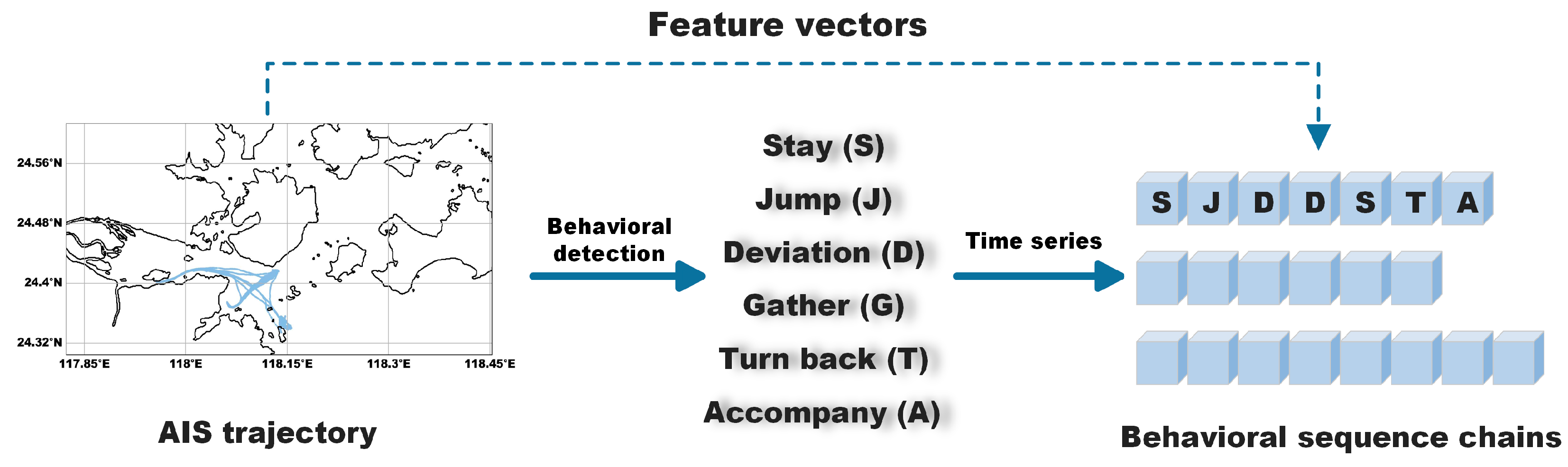
2.2. Behavioral Sequence Chain Construction

2.2.1. Behavior Symbolization and Vector Construction

The BPEF mining model provides a systematic framework for mining vessel behavior patterns and outlines the associations and combinations between different vessel behavior patterns. Next, we symbolize vessel behavior patterns by assigning a specific symbol to each pattern. For example, “S” represents stationary behavior, and “D” represents deviation from the route. This symbolic representation lays the foundation for constructing vessel behavior sequence chains. Table 2 lists the symbolic representations of vessel behavior patterns.
To accurately capture the dynamic and spatial information of each vessel behavior pattern, we assign a corresponding feature vector to each behavior pattern during the symbolic representation process. This vector is denoted as V = T , G , S , S i n θ , C o s θ . Each element in the vector represents a feature in a specific dimension, as detailed below:
  • Time Ratio (T): The time ratio represents the relative position of a specific behavioral pattern within the entire behavioral period. It normalizes the occurrence time of a behavior into the range of [0, 1]. Specifically, Tevent, Tstart, and Tend represent the absolute time of the behavioral event, the time the vessel enters the specified area, and the time it leaves, respectively, all measured in seconds. The time ratio is calculated as shown in Equation (1).
T = T e v e n t T s t a r t T e n d T s t a r t
2.
Grid encoding (G): Grid encoding represents the vessel’s geographical location by mapping its latitude and longitude coordinates to predefined grids. The area of interest is divided into fixed-size grids (e.g., 0.01° × 0.01°), and the vessel’s coordinates are assigned to the corresponding grid, producing the grid index G, This index is calculated based on the row (Row) and column (Col) indices of the grid. The specific calculation method is Equations (2)–(4).
Grid   row   index   ( Row ) =   Latitude Latitude min Grid   size  
Grid   column   index   ( Col ) = Longitude Latitude min Grid   size  
Grid   index   ( G ) = Row   ×   Total   number   of   columns + Col
3.
Speed Over Ground (S): S represents the rate at which a vessel moves per unit of time and is typically measured in knots (1 knot = 1 nautical mile/h). This value is directly obtained from AIS data.
4.
Sine and cosine values of heading angle(Sin(θ), Cos(θ)): The heading angle θ, measured in degrees and directly obtained from AIS data, is cyclic since 0° and 360° represent the same direction and is transformed into its Sin(θ) and Cos(θ) values to better capture this periodicity. The specific calculation method is outlined in Equations (5) and (6).
S i n θ = S i n 2 π × θ 360
C o s θ = C o s 2 π × θ 360

2.2.2. Behavioral Sequence Chain

Through the BPEF mining model in Section 2.1 of this paper, we mine all behavior patterns of the target vessel and known anomalous vessels, converting them into corresponding behavior symbols as described in Section 2.2.1. Then, based on the temporal sequence combination of vessel behavior patterns, all behavior pattern symbols are sorted by occurrence time, and the feature vectors of each behavior pattern are similarly ordered, ultimately forming a vessel behavior sequence chain with associated feature vectors. The specific construction process of the ship behavior sequence chain is shown in Figure 3.

2.3. Anomaly Detection

After constructing the vessel behavior sequence chain, the similarity between the target vessel’s behavior sequence and that of anomalous vessels is compared. We propose an improved Jaro–Winkler similarity algorithm to calculate the similarity between locally optimal matching sequences aligned by the Smith–Waterman algorithm. Additionally, to reduce the impact of sequence completeness on anomaly detection results, we apply the LCS method to evaluate the integrity of the behavior sequence chains. Next, we apply an alternating optimization method to determine three weight parameters and an anomaly threshold. Using these parameters, we calculate the overall similarity between vessel behavior sequence chains. Finally, anomalous vessels are identified by comparing the combined similarity with the anomaly threshold.

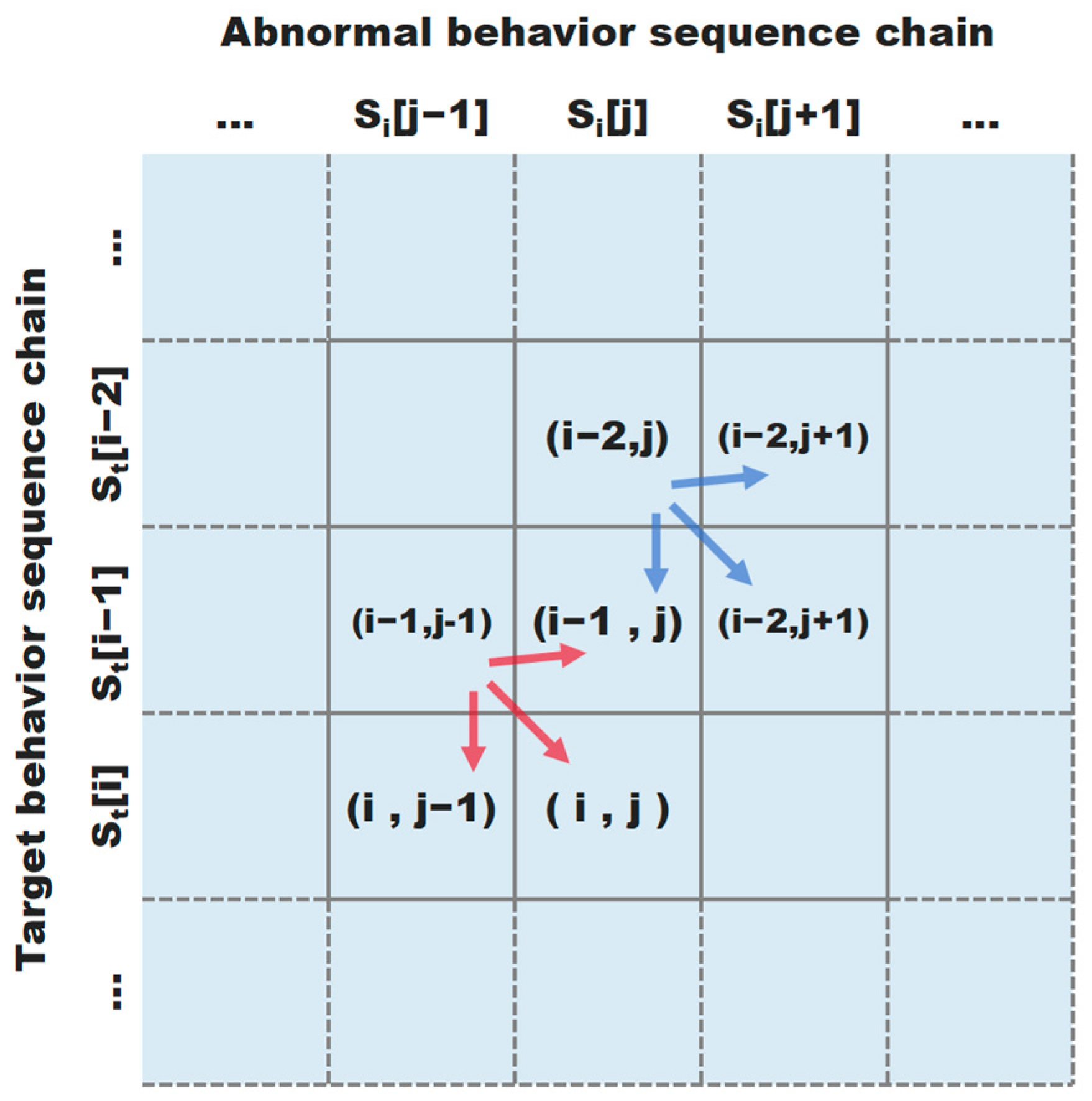
2.3.1. Smith–Waterman Local Alignment

The Smith–Waterman algorithm is a dynamic programming method widely used for local sequence alignment in bioinformatics. It constructs a dynamic programming matrix to evaluate all possible alignments and determine the optimal local alignment. In this study, the algorithm is applied to locally align the behavior sequence chains of the target vessel and anomalous vessels. By optimizing the scoring matrix and considering matches, mismatches, insertions, and deletions, the best local alignment between the two sequence chains is determined through backtracking of the score matrix.
We select the behavioral sequence chains S1 from the target vessel and S2 from the anomalous vessel, with lengths m = S 1 and n = S 2 , respectively. We construct a score matrix D of size m + 1 × n + 1 , where each cell represents the best alignment score up to that position. For each character pair in the two sequences, (1) we assign a match score of m = 3 if the characters match; (2) we apply a mismatch penalty of d = 3 if the characters do not match; and (3) we introduce gaps in the sequences to account for misalignments, with a gap penalty of g = 2 . A dynamic programming algorithm populates the score matrix D. Each cell’s value is determined by the maximum of four possible calculations: (1) The value from the diagonal cell plus the match score if the characters match or the mismatch penalty if they do not; (2) the value from the cell above, incremented by the gap penalty g; (3) the value from the cell to the left, incremented by the gap penalty g; and (4) a value of 0, indicating the start of a new local alignment.
Equation (7) and Figure 4 provide a detailed illustration of the computational steps involved in the Smith–Waterman algorithm.
D ( i , j ) = D ( i 1 , j 1 ) + s ( S t [ i ] , S i [ j ] ) D ( i 1 , j ) + g D ( i , j 1 ) + g 0
The score matrix initializes to zero, representing gaps at the start of the sequences and allowing local alignments to begin at any position within the chains. After filling all the cells, the highest value in the matrix D marks the endpoint of the optimal local alignment. Backtracking starts at this maximum value and continues towards the top-left corner, stopping when a cell with a value of 0 is reached. During backtracking, the optimal alignment is determined by these rules: (1) Move to the diagonal cell if the current cell originates from there and the characters match or mismatch; (2) move to the cell above if the current cell originates from it; and (3) move to the cell to the left if the current cell originates from it. For example, Figure 5 demonstrates the Smith–Waterman algorithm’s local alignment between the test sequence TGTTSCGG and the anomalous chain GGTTGSCTS. First, the score matrix is constructed and filled step-by-step, as shown in Figure 5a. Next, the highest value in the matrix is identified, marking the alignment’s endpoint. Following the backtracking rules, the process proceeds from this point, as shown in Figure 5b. Figure 5c highlights the most similar local regions, with vertical lines “|” representing matches and hyphens “-” indicating gaps.

2.3.2. Similarity Calculation

The similarity calculation between vessel behavior sequence chains consists of two parts: local similarity and comprehensive similarity. First, we propose an improved Jaro–Winkler algorithm to evaluate the local similarity between vessels, used to calculate the similarity between behavior sequence subsequences aligned by the Smith–Waterman algorithm. The Jaro–Winkler algorithm is a method for calculating the similarity between two strings, derived from the Jaro algorithm. The higher the score, the greater the similarity between the two strings, with a score of “1” indicating a perfect match and a score of “0” indicating no similarity. This algorithm is particularly suitable for calculating the similarity between short strings (such as behavior sequence subsequences) due to its high accuracy and efficiency when handling shorter strings.
The two aligned behavioral sequence sub-chains are denoted as S1′ and S2′, and the Jaro–Winkler similarity between them is computed using the formula in Equations (8) and (9). Specifically, M represents the sum of all match scores between behavioral sub-sequence chains, while |S1′| and |S2′| represent the lengths of strings S1′ and S2′. The term t refers to half the number of transpositions (e.g., if S1′ and S2′ have 6 matching characters, with 2 out of order, then t = 1). The factor P is the weighting factor (typically 0.1), and L represents the length of the common prefix, with a maximum value of 4.
J a r o = 1 3 ( M S 1 + M S 2 + M t M )
J a r o W i n k l e r = J a r o + P × L × 1 J a r o
In the original Jaro–Winkler algorithm, the match score M between two strings increases by 1 only when characters match. In our improved algorithm, we first filter all successfully matched character pairs based on the match threshold R (Equation (10)) and add them to the match set Mset (Equation (11)). Here, S1i′ and S2j′ ∈ Mset represent the character pairs in the match set. The match threshold R defines the maximum allowable distance between matching characters in the two behavior subsequence chains. Next, we extract each matching character pair and its corresponding feature vectors V1i and V2j from the match set Mset and compute the Mahalanobis distance between them (Equation (12)). This calculation provides a more precise match score for each character pair.
R = max ( S 1 , S 2 ) 2 1
M s e t = S 1 i , S 2 j S 1 i = S 2 j , i j R
D M ( V 1 i , V 2 j ) = ( V 1 i V 2 j ) T Σ 1 ( V 1 i V 2 j )
To prevent the direct summation of Mahalanobis distances from disproportionately affecting the overall similarity, we normalize all Mahalanobis distances (Equation (13)). After normalization, all distances are scaled to the [0, 1] range, eliminating biases caused by feature dimension differences and ensuring that each matching character pair contributes more fairly and consistently. Finally, we sum all the normalized Mahalanobis distances to obtain the final match score M (Equation (14)), providing a more accurate measure of the behavior pattern matching between the behavior subsequence chains.
D M n o r m ( S 1 i , S 2 j ) = D M ( S 1 i , S 2 j ) D m i n D max D min
M = ( S 1 i , S 2 j ) M s e t D M n o r m ( S 1 i , S 2 j )
We use the improved match score M to calculate the Jaro–Winkler similarity, thereby obtaining the similarity Slocal between the target behavior subsequence and the anomalous behavior subsequence.
In the similarity calculation of behavior sequence chains, not only the similarity between the aligned behavior subsequences needs to be considered, but also the degree of change in the sequence chain, i.e., the completeness of the sequence chain. This completeness measure evaluates whether the characteristics of the original behavior sequence chain are adequately preserved during the registration process to prevent over-trimming, which could cause sequence bias and impact the reliability of the similarity calculation. To fully consider the impact of behavior sequence chains on the anomaly detection results, we introduce the LCS to mitigate the bias caused by information loss and quantify the integrity of the sequence chain. The LCS values of the target sequence chain completeness and the anomalous sequence chain completeness are denoted as Sself-1 and Sself-2, respectively.
Next, we propose a weighted composite similarity method to further improve the accuracy and reliability of the anomaly detection results. This method combines local similarity Slocal, target sequence chain completeness Sself-1, and anomalous sequence chain completeness Sself-2, assessing the similarity between the target and the known anomalous sequence chains from multiple dimensions. Specifically, Slocal represents the local similarity after alignment, i.e., the similarity between the behavior subsequences, while Sself-1 and Sself-2 reflect the completeness measures of the target and anomalous sequence chains, respectively. Finally, the calculation formula for the composite similarity Scomp is as follows:
S c o m p = A × S l o c a l + B × S s e l f 1 + C × S s e l f 2
where A, B, and C are weighting coefficients used to adjust the relative importance of each similarity measure in the overall evaluation.

2.3.3. Adaptive Parameter Adjustment

This study employs an alternating optimization method to adjust the weights and thresholds. The weights A, B, and C reflect the contributions of different similarity measures to the comprehensive similarity, while the threshold determines whether the comprehensive similarity meets the anomaly detection standard. The specific optimization process involves initially setting the weights and thresholds. The initial threshold is determined by the quantile (e.g., 75% or 85%) of the local similarity between known anomalous ship behavioral sequence chains, and multiple initial weight parameters are set based on the importance of different features.
In each iteration, the weights are optimized while the threshold is fixed, followed by the optimization of the threshold with the weights fixed. This process is repeated until the detection performance of the model stabilizes, ensuring a detection efficiency of 95% or higher. After determining the threshold and weights, the anomaly standards for ships are established based on the comprehensive similarity. The comprehensive similarity Scomp is compared to the predefined threshold:
If Scomp ≥ threshold, the target ship’s behavior is considered highly similar to anomalous behavior, and the ship is classified as anomalous.
If Scomp < threshold, the target ship’s behavior does not meet the anomaly similarity standard, and the ship is classified as normal.

2.4. Mainstream Algorithms for Ship Anomalous Behavior Detection

To demonstrate the effectiveness of the BPEF-TSD framework, we compared its performance with several representative anomaly detection algorithms, including LSTM (long short-term memory), iForest (isolation forest), and HDBSCAN (hierarchical density-based spatial clustering of applications with noise) algorithms. The details of these algorithms can be found as follows:

2.4.1. LSTM

LSTM is a specialized recurrent neural network (RNN) recognized for its strong performance in sequence-based tasks and is particularly well-suited for anomaly detection in time series data. By incorporating gating mechanisms such as the input gate, forget gate, and output gate, LSTM dynamically regulates the retention and discarding of information, addressing the gradient vanishing problem in traditional RNNs and effectively capturing long-term dependencies in time series data. The specific formula is as follows:
C t = f t · C t 1 + i t · C ~ t
h t = o t · t a n h C t
where Ct is the current memory state; Ct−1 is the memory state from the previous step; it is the input gate output, determining how much new information to add, with it ∈ [0, 1]; C ~ t is candidate memory content, representing new input information, with C ~ t ∈ [−1, 1]; ot is output gate output, deciding how much of the memory state to reveal, with ot ∈ [0, 1]; ht is the hidden state, representing the current output of the LSTM cell; and tanh is the activation function used to scale values between [−1, 1].

2.4.2. iForest

The iForest method is based on the concept of “isolation” and constructs isolation trees by randomly selecting attributes and partitioning points to separate anomalous data. Inspired by the random forest approach, iForest is an unsupervised anomaly detection technique that operates on the core principle: “Outliers are more easily isolated”. This method integrates the temporal and spatial characteristics of AIS data, enabling it to effectively detect anomalies in both clustered and dispersed regions. iForest demonstrates exceptional computational efficiency when applied to high-dimensional datasets and reliably isolates anomalies, making it a powerful tool for anomaly detection. The specific formula is as follows:
s x , n = 2 E h x c n
c n = 2 l n n 1 + γ 2 n 1 n
where n is the number of samples in the dataset; s x , n is the anomaly score of sample x, with s x , n   ∈ [0, 1]; E h x is the expected path length of sample x, representing the number of splits needed to isolate x in the isolation tree; c n is a normalization factor for the average path length in a dataset of size n; and γ is Euler’s constant (approximately 0.577).

2.4.3. HDBSCAN

HDBSCAN effectively addresses challenges associated with uneven data distribution. This advanced density-based clustering algorithm excels in detecting trajectory points with abnormal density distributions. Constructing a minimum spanning tree represents the hierarchical relationships between points, while sparse points are identified as noise based on a predefined density threshold. Points with low density are classified as anomalies. The specific formula is as follows:
c o r e _ d i s t p = d i s t a n c e p ,   k t h   n e a r e s t   n e i g h b o r
m r e a c h p , q = m a x c o r e _ d i s t p , c o r e _ d i s t q , d i s t a n c e p , q
where m r e a c h p , q is the mutual reachability distance between points p and q, which reflects their local density relationship; c o r e _ d i s t p and c o r e _ d i s t q are the core distances of p and q, defining their local density; and d i s t a n c e p , q is the direct distance between points p and q.

2.5. Evaluation Metrics

We evaluate the results based on the true labels of AIS data, the artificially labeled generated trajectories, and the predicted labels. The primary goal of anomaly detection is to improve the detection accuracy for the minority anomalous class. To assess the efficiency and accuracy of the BPEF-TSD anomaly detection framework, we use four evaluation metrics: accuracy (Acc), precision (P), recall (R), and F1-score. The formulas for calculating these metrics are as follows.
A c c = T N + T P T N + T P + F N + F P
P = T P T P + F P
R = T P T P + F N
F 1 = 2 × P × R P + R
In the formula, TP refers to true positives (correctly detected normal samples); TN refers to true negatives (correctly detected anomalous samples); FP refers to false positives (anomalous samples incorrectly detected as normal); and FN refers to false negatives (normal samples misclassified as anomalous). Acc measures the model’s overall detection accuracy. P represents the precision in detecting positive samples, while R evaluates the proportion of correctly identified positive samples. The F1-score balances P and R, addressing the impact of class imbalances that can distort their values.

3. Experiments and Results

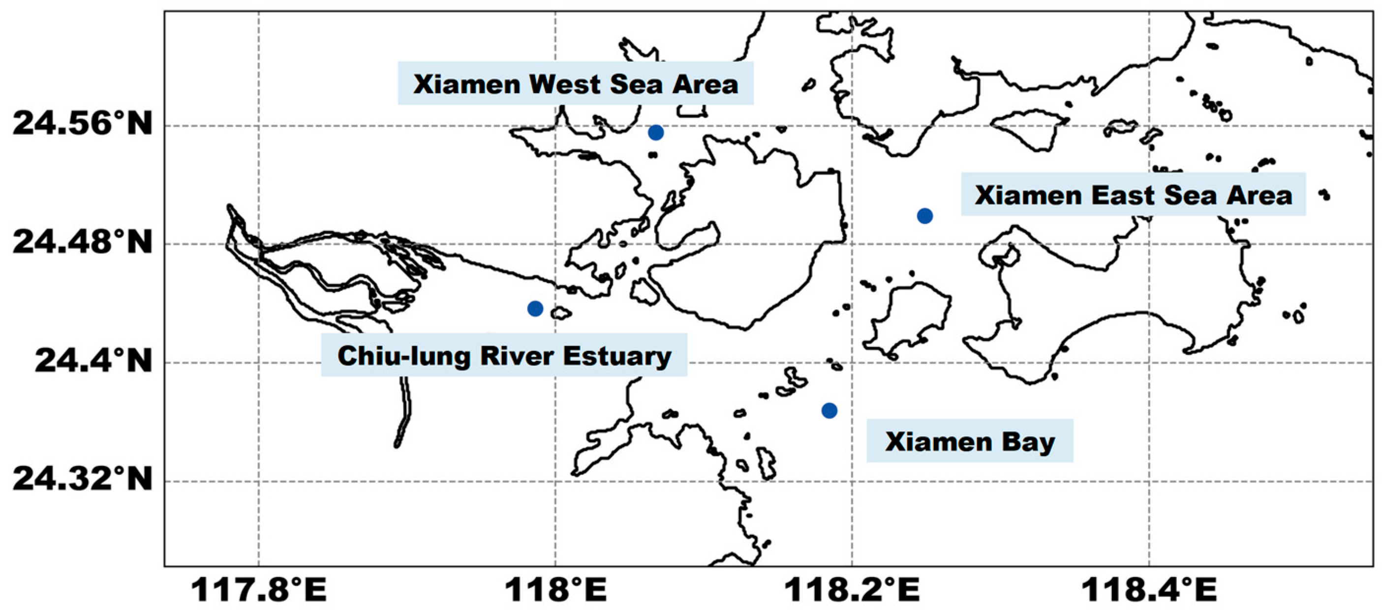
3.1. Study Area and Experimental Setup

We selected Xiamen Port and its surrounding waters as the experimental area for this study. Situated on the southeast coast of China, Xiamen Port is located at 118°04′ east longitude and 24°27′ north latitude, as shown in Figure 6. It is one of China’s significant coastal ports and serves as a key hub in the national transportation network. This study collected AIS data from Xiamen Port and its surrounding waters between 12 October and 31 December 2022, covering a geographical range of 24.30° to 24.60° north latitude and 117.80° to 118.45° east longitude, as shown in Figure 7. Within this study area, the average ship speed was 5.8 knots, with speeds ranging from 0 to 18.5 knots, and the average time interval between trajectory points was 2 min. After data cleaning and preprocessing, a total of 13,512 ship trajectories were obtained. To ensure the representativeness and reliability of model training and evaluation, the dataset was divided into a training set, validation set, and test set in a ratio of 3:1:1. The training set was used for model parameter learning, the validation set for optimizing hyperparameters, and the test set for evaluating model performance.
In maritime traffic, the number of ship behavior samples with anomaly labels is limited, and there is insufficient knowledge of potential anomalous behaviors. In order to obtain more trajectories of anomalous ship behavior, we need to mix anomalous behavior with known normal behavior. Consequently, this study introduces a method for generating anomalous trajectories based on existing AIS data. The steps involved are as follows:
First, we randomly select a trajectory from normal behavior samples and choose a random point within it as the starting point for behavior. From this point, a random navigation mode is selected based on the behavior pattern definitions. In each mode, randomly generated course and speed values fall within the ranges of 0–360° and 0–20 knots, respectively, and the navigation trajectory is simulated according to the behavior pattern’s characteristics. The duration of each behavior pattern is randomly determined within a specified range, and each anomalous trajectory may consist of multiple behavior patterns. To ensure diversity and plausibility, the occurrence of any behavior pattern in a single trajectory is limited to three times. Using this method, we generate a single anomalous trajectory. Two hundred anomalous trajectories were generated for each subset of the training dataset and the evaluation dataset.

3.2. Experimental Results and Analysis

3.2.1. Optimal Model Input Parameters Selection

Using the known anomalous ship behavior data in the training dataset, we first calculated the similarity distribution of ship behaviors among anomalous ships. Figure 8 illustrates that the similarity scores of anomalous ships are primarily distributed between 0.4 and 0.9, indicating a notable degree of behavioral similarity among anomalous ships. According to the similarity scores, a range of potential thresholds was established to balance detection accuracy and false positive rates. Here, we set the initial threshold as the 75th and 85th percentiles based on the statistical results, as these quantiles effectively represent the majority of anomalous behavior characteristics, ensuring both the sensitivity and precision of the model.
We conducted six experimental combinations with varying weight parameters (A, B, and C) and two initial similarity thresholds (75th and 85th percentiles) to explore the impact of these factors on anomaly detection performance. The different combinations were designed to assess how the relative importance of each similarity measure and the choice of threshold affect the overall detection accuracy, as follows: (1) A = 0.5, B = 0.25, C = 0.25, threshold = 0.73; (2) A = 0.5, B = 0.25, C = 0.25, threshold = 0.77; (3) A = 0.25, B = 0.5, C = 0.25, threshold = 0.73; (4) A = 0.25, B = 0.5, C = 0.25, threshold = 0.77; (5) A = 0.25, B = 0.25, C = 0.5, threshold = 0.73; and (6) A = 0.25, B = 0.25, C = 0.5, threshold = 0.77. We tested multiple weight configurations and threshold values to identify the optimal balance for distinguishing normal and anomalous vessel behaviors. The final model parameters were selected based on the average results from these experiments.
Figure 9a–f illustrates the dynamic trends of parameter A and parameters B and C under various parameter combinations and similarity threshold conditions. Across all combinations, parameter A exhibits an overall upward trend and consistently dominates, highlighting the critical role of local similarity in anomaly detection. Conversely, parameters B and C demonstrate a consistent downward trend, with their rates of decline and fluctuation characteristics influenced by the initial weight configuration and threshold selection. For the combination with initial weights A = 0.5, B = 0.25, and C = 0.25, as shown in Figure 9a,b. Parameter A undergoes a rapid initial adjustment followed by a significant increase, while parameters B and C decrease more gradually. This behavior indicates that the model progressively strengthens the weight of local similarity, emphasizing its priority. In contrast, when the initial weight of B or C is higher, as depicted in Figure 9c–f, parameters B or C decline more rapidly, whereas parameter A increases at a slower rate. In Figure 9d,f, where the initial weight of parameter B or C is the highest, the model initially relies on the integrity feature. However, as iterations progress, the weight of the local similarity feature A rises rapidly and eventually dominates, demonstrating the model’s ability to dynamically adjust feature weights for optimizing anomaly detection. Notably, in Figure 9f, parameter A experiences a significant drop around the 80th iteration, likely due to the objective function nearing convergence. During this stage, the model may make substantial weight adjustments to explore potentially better solutions, resulting in short-term fluctuations in local similarity weights. Nevertheless, parameter A recovers quickly and continues its upward trajectory, reaffirming the central importance of local similarity in the final optimization process.
We further analyzed the validity of the threshold in our method framework. As shown in Figure 10, the experimental results indicate that the threshold distribution exhibits significant regularity and adaptability under different combination modes. In Figure 10a,b,d,e, the threshold distribution exhibits a multi-modal characteristic, suggesting the model’s ability to flexibly explore multiple potential optimal ranges under complex conditions, thereby demonstrating strong adaptability. In Figure 10c,f, the threshold distribution is closer to unimodal, indicating that the model achieves greater focus and convergence under these conditions. Additionally, the threshold density is generally concentrated around 0.75, suggesting that this range may represent the optimal solution across multiple combinations. The secondary peaks in different combinations reflect the model’s ability to dynamically adjust based on varying scenarios.

3.2.2. Dynamic Trends and Validation of Model Performance Indicators

Figure 11a–f illustrates the dynamic changes in the model’s four performance indicators under various initial weight parameters and threshold settings. Across all combinations, the indicators generally follow a pattern of “slow growth in the early stage, rapid improvement in the middle stage, and stabilization in the late stage”. Specifically, Figure 11a,b show that accuracy and precision remain particularly stable during the middle stage and reach near-convergence in the late stage. In contrast, Figure 11c,d indicate more pronounced fluctuations in recall, especially during the early stage when the model’s ability to detect anomalous behavior is still developing. Figure 11e highlights significant improvements across all four indicators, with the F1-score exhibiting particularly notable growth. This pattern suggests that the model progressively enhances its ability to capture the local similarity of anomalous behavior as the influence of self-integrity features diminishes. Notably, in all combinations, although the overall performance of the indicators is strong, slight fluctuations occur during the later stage, around the 80th iteration, likely due to the fine-tuning of local feature weights. Additionally, the consistently high F1-scores across multiple combinations confirm the model’s ability to accurately identify abnormal behaviors and minimize missed detections, ensuring its reliability and adaptability for practical applications in diverse scenarios.
Figure 12a presents a radar chart comparing the optimal parameter combinations from six experiments conducted on the training dataset. The results indicate that the model maintains high recall and precision across different parameter configurations, with stable detection outcomes. Based on the optimization results from the training dataset, we set the weight parameters to 0.6, 0.2, and 0.2, and the threshold to 0.75. We then validated the model using the Xiamen Port test dataset. As shown in Figure 12b, the BPEF-TSD demonstrates outstanding performance across four metrics: precision, recall, F1-score, and accuracy. Specifically, the model achieves a precision of 0.964, a recall of 0.928, an F1-score of 0.945, and an accuracy of 0.910.

3.2.3. Comparative Experiment with Mainstream Algorithms

We conducted comparative experiments, and the results are presented in Table 3. Four methods, BPEF-TSD, LSTM, iForest, and HDBSCAN, were evaluated using four performance indicators: precision, recall, F1-score, and accuracy. The results indicate that BPEF-TSD significantly outperforms the other methods in overall performance. Specifically, BPEF-TSD achieved precision, recall, and F1-score values of 0.964, 0.928, and 0.945, respectively, which are higher than those of the other methods, demonstrating an effective balance between precision and recall. Although HDBSCAN exhibits the highest accuracy, its anomaly detection capability is limited, with precision and recall values of only 0.347 and 0.520, respectively. In contrast, BPEF-TSD demonstrates superior detection efficiency and accuracy, particularly in recognizing complex behavior patterns and detecting anomalies. These results validate the effectiveness and robustness of the BPEF-TSD framework in detecting abnormal ship behavior, providing critical support for maritime safety supervision.

4. Discussion

The test results indicate that, with appropriate weight and threshold configurations, the model can effectively detect anomalous behaviors and is suitable for the vessel anomaly detection task in the Xiamen Port area. However, during the course of this experiment, we identified certain limitations in the anomaly detection methods based on vessel behavior patterns.
  • Over-reliance on AIS data quality: During the experiment, we observed that the BPEF-TSD method is heavily dependent on the quality of AIS data, and its performance is limited by the available anomalous vessel data. AIS data integrity is essential for accurately capturing vessel behavior patterns, but the small number of anomalous data samples restricts model training and validation. To address the lack of real-world anomalous data, we introduced a synthetic data generation method that combines normal and anomalous behaviors, enhancing the dataset and model robustness. However, synthetic data may not fully capture the complexities of real-world anomalies, which could impact detection accuracy in actual maritime environments [40]. In the future, we can employ data augmentation techniques, such as SMOTE, to increase the number of anomalous samples [41,42]. Additionally, data fusion techniques can be used to integrate other data sources, such as radar, satellite imagery, and optical sensors, reducing reliance on a single data source and improving the accuracy and reliability of the detection process [43,44].
  • Generalizability of the Xiamen Port data: This study focuses on Xiamen Port, a key coastal and container port in China. However, the methods we developed are designed to be adaptable to other maritime environments. We selected Xiamen Port because it represents typical maritime behaviors, such as navigation, docking, and cargo handling. The BPEF-TSD framework, built on general principles of ship behavior, can be applied to other ports or waterways with similar conditions. By leveraging behavioral patterns, similarity measures, and anomaly detection algorithms, the framework demonstrates broad applicability. In future work, we plan to further test and validate the framework using data from other waterways. This will enable us to evaluate its effectiveness across a wider range of maritime environments, ensuring that the proposed anomaly detection system is not only suitable for Xiamen Port but also adaptable to various maritime contexts.
  • Limited applicability to multi-vessel scenarios: The BPEF-TSD method primarily targets the behavior patterns of individual vessels and does not fully account for multi-vessel coexistence scenarios, such as escorting or overtaking. This limitation reduces the method’s effectiveness in areas with frequent vessel interactions [45]. Future research could expand the behavior pattern recognition algorithm to analyze collective vessel behavior, enhancing its ability to recognize complex patterns such as group navigation and strategic avoidance [46,47].
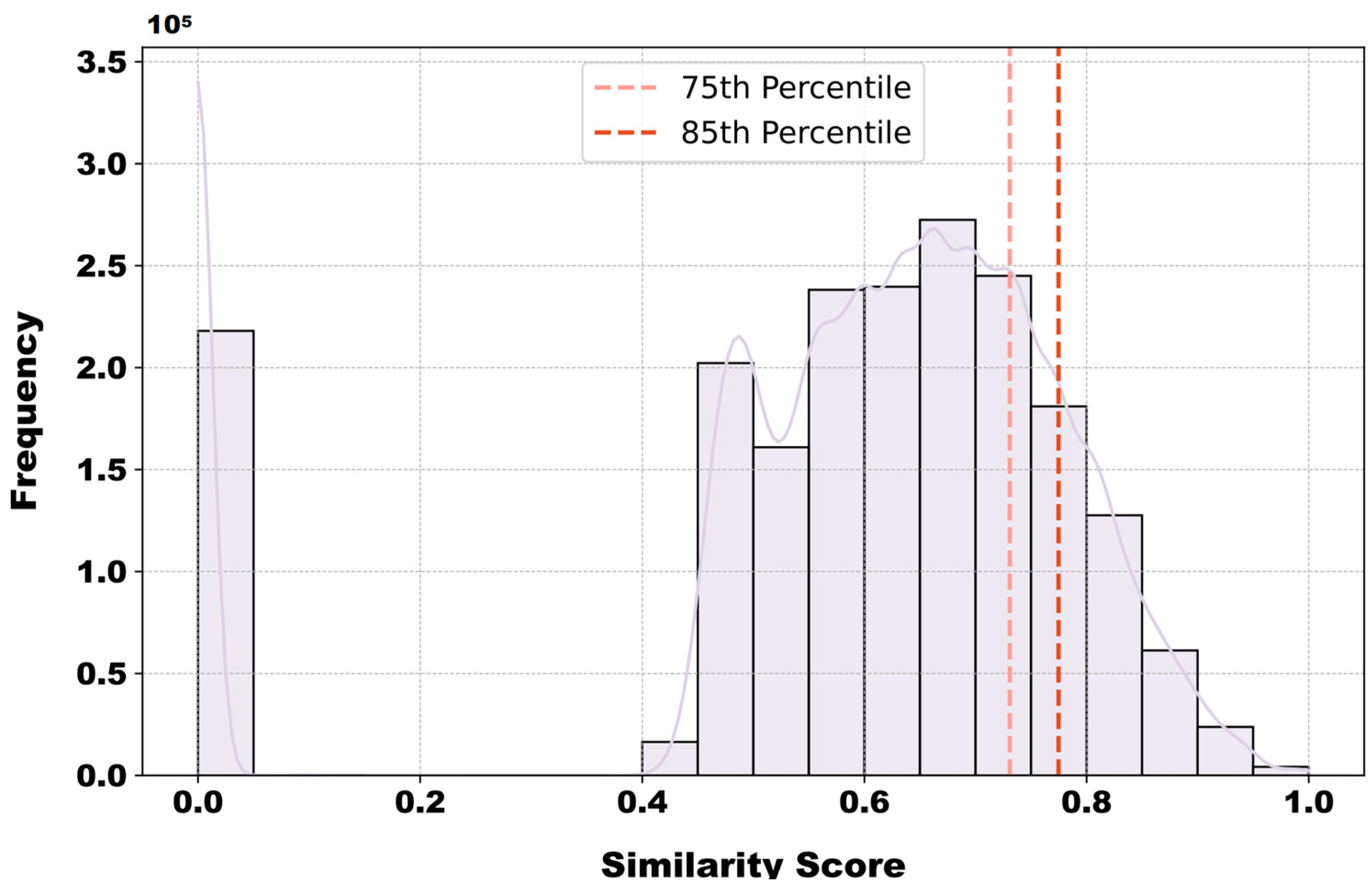
  • Challenges in threshold setting: In this study, we used a single threshold for anomaly behavior detection. In practical applications, the complexity of data characteristics and scenarios may render a fixed threshold unsuitable for all cases. Specifically, both excessively high and low thresholds can lead to incorrect anomaly detection. Previous studies have explored this issue, highlighting that the selection of an appropriate threshold should consider both data characteristics and the application scenario [48]. In the future, adaptive threshold techniques could be considered to dynamically adjust thresholds based on real-time data, or machine learning methods could be employed to automatically learn the optimal threshold, potentially improving detection sensitivity and accuracy [49].

5. Conclusions and Future Work

This study introduces a vessel anomaly detection framework based on BPEF mining and text similarity, designed to identify and detect target vessels that exhibit behavior patterns similar to known anomalous vessels during navigation. Our method utilizes BPEF mining to extract vessel behavior events and construct behavior sequence chains. We apply the Smith–Waterman algorithm to locally align the behavior sequence chains of target vessels with those of known illegal vessels, identifying the most similar local segments. Subsequently, we enhance the Jaro–Winkler text similarity algorithm and combine it with the LCS algorithm to calculate the overall similarity between the behavior sequence chains of target vessels and known illegal vessels, effectively identifying potential risk vessels.
Experimental results demonstrate that this detection method maintains high precision and recall while delivering stable detection outcomes under appropriate weight parameters and threshold configurations. Compared to manually annotated anomalous trajectory points, our proposed method achieves an accuracy exceeding 95% in identifying anomalous behaviors. This further validates that appropriate parameter adjustments enable the model to sustain high detection performance in real-world scenarios, providing efficient and reliable technical support for maritime safety supervision and showcasing its engineering application potential in maritime anomaly detection.
In future research, we could incorporate longer time span ship trajectory data to improve the accuracy of navigation pattern recognition. Additionally, integrating multi-source data, such as radar, satellite imagery, and environmental conditions, into the BPEF mining framework would enable a more comprehensive capture of ship behavior, thereby enhancing the robustness and accuracy of anomaly detection. Moreover, exploring adaptive thresholding mechanisms and improved data fusion techniques could better handle noisy or missing data, ensuring more reliable results. Finally, upon detecting anomalous behaviors, developing supplementary regulatory tools capable of swiftly identifying the causes of anomalies and mitigating false positives from normal navigation adjustments would further optimize maritime safety management.

Author Contributions

Conceptualization, Y.S., Y.W. and L.C.; methodology, Y.W.; software, Y.W.; validation, Y.S. and Y.W.; formal analysis, Y.W.; data curation, Y.W.; writing—original draft preparation, Y.W.; writing—review and editing, Y.W. and L.C.; funding acquisition, Y.S. All authors have read and agreed to the published version of the manuscript.

Funding

This work was supported by Natural Science Foundation of Xiamen, China (No. 3502Z202473059), the Chunhui Project Foundation of the Education Department of China (No. 202200324), the National Natural Science Foundation of China (No. 52371369), the Key Projects of National Key R & D Program (No. 2021YFB390150), the Natural Science Project of Fujian Province (No. 2022J01323, 2021J01822, 2020J01660, 20230019), the Fuzhou-Xiamen-Quanzhou Independent Innovation Region Cooperated Special Foundation (No. 3502ZCQXT2021007).

Institutional Review Board Statement

Not applicable.

Informed Consent Statement

Not applicable.

Data Availability Statement

The datasets presented in this article are not readily available because the data are subject to copyright restrictions by the data provider and can only be accessed upon request or after the decryption period. Requests to access the datasets should be directed to 202212861028@jmu.edu.cn.

Conflicts of Interest

The authors declare no conflicts of interest.

References

  1. Xin, X.; Liu, K.; Loughney, S.; Wang, J.; Yang, Z. Maritime Traffic Clustering to Capture High-Risk Multi-Ship Encounters in Complex Waters. Reliab. Eng. Syst. Saf. 2023, 230, 108936. [Google Scholar] [CrossRef]
  2. Durlik, I.; Miller, T.; Dorobczyński, L.; Kozlovska, P.; Kostecki, T. Revolutionizing Marine Traffic Management: A Comprehensive Review of Machine Learning Applications in Complex Maritime Systems. Appl. Sci. 2023, 13, 8099. [Google Scholar] [CrossRef]
  3. Li, B. Multi-Feature Fusion Anomaly Detection Model Based on Ship Behavior Analysis; Dalian Maritime University: Dalian, China, 2022. [Google Scholar]
  4. Wang, L.; Chen, P.; Chen, L.; Mou, J. Ship Ais Trajectory Clustering: An Hdbscan-Based Approach. J. Mar. Sci. Eng. 2021, 9, 566. [Google Scholar] [CrossRef]
  5. Chen, Y.; Yang, S.; Suo, Y. Research Progress of Ship Behavior Anomaly Detection. J. Transp. Inf. Saf. 2020, 38, 1–11. [Google Scholar]
  6. Tang, H.; Yin, Y.; Shen, H. Survey of Abnormal Behavior of Marine Vessels. J. Chongqing Jiaotong Univ. Nat. Sci. 2019, 38, 109–115. [Google Scholar]
  7. Zhang, B.; Ren, H.; Wang, P.; Wang, D. Research Progress on Ship Anomaly Detection Based on Big Data. In Proceedings of the 2020 IEEE 11th International Conference on Software Engineering and Service Science (ICSESS), Beijing, China, 16–18 October 2020; pp. 316–320. [Google Scholar]
  8. Rong, H.; Teixeira, A.P.; Guedes Soares, C. Data Mining Approach to Shipping Route Characterization and Anomaly Detection Based on Ais Data. Ocean Eng. 2020, 198, 106936. [Google Scholar] [CrossRef]
  9. Yu, S.; Zhou, H.; Ye, C.; Wang, T. Sdfa: Study on Ship Trajectory Clustering Method Based on Multi-Feature Fusion. Comput. Sci. 2022, 49, 250–260. [Google Scholar]
  10. Wei, H.; Chen, Z.; Zhang, L. Anomaly Detection Framework of System Call Trace Based on Sequence and Frequency Patterns. Comput. Sci. 2022, 49, 350–355. [Google Scholar]
  11. Zhou, Y.; Damen, W.; Vellinga, T.; Hoogendoorn, S.P. Ship Classification Based on Ship Behavior Clustering from Ais Data. Ocean Eng. 2019, 175, 176–187. [Google Scholar] [CrossRef]
  12. Sun, S.; Chen, Y.; Zhang, J. Trajectory Outlier Detection Algorithm for Ship Ais Data Based on Dynamic Differential Threshold. J. Phys. Conf. Ser. 2020, 1437, 012013. [Google Scholar]
  13. Yang, A.; Chang, X.; Zhang, Q.; Zhao, F. Abnormal Behavior Detection of Ships in Sensitive Water Area Based on Ais Data. Command. Inf. Syst. Technol. 2023, 14, 32–37. [Google Scholar]
  14. Xie, Z.; Bai, X.; Xu, X.; Xiao, Y. An Anomaly Detection Method Based on Ship Behavior Trajectory. Ocean Eng. 2024, 293, 116640. [Google Scholar] [CrossRef]
  15. Yin, C.; Zhang, S.; Wang, J.; Xiong, N.N. Anomaly Detection Based on Convolutional Recurrent Autoencoder for Iot Time Series. IEEE Trans. Syst. Man Cybern. Syst. 2022, 52, 112–122. [Google Scholar] [CrossRef]
  16. Czaplewski, B.; Dzwonkowski, M. A Novel Approach Exploiting Properties of Convolutional Neural Networks for Vessel Movement Anomaly Detection and Classification. ISA Trans. 2022, 119, 1–16. [Google Scholar] [CrossRef] [PubMed]
  17. Wang, Z.; Zhao, K.; Cai, C.; Ding, M.; Wang, P. Analysis of Vessel Abnormal Behavior Based on Dbscan and Iforest Algorithms. Ship Electron. Eng. 2021, 41, 89–94. [Google Scholar]
  18. Wang, F.; Lei, Y.; Liu, Z.; Wang, X.; Ji, S.; Tung, A.K.H. Fast and Parameter-Light Rare Behavior Detection in Maritime Trajectories. Inf. Process. Manag. 2020, 57, 102268. [Google Scholar] [CrossRef]
  19. Shi, Y.; Long, C.; Yang, X.; Deng, M. Abnormal Ship Behavior Detection Based on Ais Data. Appl. Sci. 2022, 12, 4635. [Google Scholar] [CrossRef]
  20. Liu, H.; Wang, Y.; Chen, W. Anomaly Detection for Condition Monitoring Data Using Auxiliary Feature Vector and Density-Based Clustering. IET Gener. Transm. Distrib. 2019, 14, 108–118. [Google Scholar] [CrossRef]
  21. Pallotta, G.; Vespe, M.; Bryan, K. Vessel Pattern Knowledge Discovery from Ais Data: A Framework for Anomaly Detection and Route Prediction. Entropy 2013, 15, 2218–2245. [Google Scholar] [CrossRef]
  22. Zhao, L.; Shi, G. Maritime Anomaly Detection Using Density-Based Clustering and Recurrent Neural Network. J. Navig. 2019, 72, 894–916. [Google Scholar] [CrossRef]
  23. Singh, S.K.; Fowdur, J.S.; Gawlikowski, J.; Medina, D. Leveraging Graph and Deep Learning Uncertainties to Detect Anomalous Maritime Trajectories. IEEE Trans. Intell. Transp. Syst. 2022, 23, 23488–23502. [Google Scholar] [CrossRef]
  24. Karataş, G.B.; Karagoz, P.; Ayran, O. Trajectory Pattern Extraction and Anomaly Detection for Maritime Vessels. Internet Things 2021, 16, 100436. [Google Scholar] [CrossRef]
  25. Jin, L.; Luo, Z.; Gao, S. Visual Analytics Approach to Vessel Behavior Analysis. J. Navig. 2018, 71, 1195–1209. [Google Scholar] [CrossRef]
  26. Coleman, J.; Kandah, F.; Huber, B. Behavioral Model Anomaly Detection in Automatic Identification Systems (Ais). In Proceedings of the 2020 10th Annual Computing and Communication Workshop and Conference (CCWC), Las Vegas, NV, USA, 6–8 January 2020; pp. 481–487. [Google Scholar]
  27. Tang, H.; Wei, L.; Yin, Y.; Shen, H.; Qi, Y. Detection of Abnormal Vessel Behavior Based on Probabilistic Directed Graph Model. J. Navig. 2020, 73, 1014–1035. [Google Scholar] [CrossRef]
  28. He, F.; He, Z.; Yang, F.; Liu, L. Research on Recognition Method of Abnormal Behavior of Ships Based on Electronic Chart. J. Wuhan Univ. Technol. Transp. Sci. Eng. 2019, 43, 631–636+645. [Google Scholar]
  29. Bao, L. A Trajectory Data Anomaly Detection Method Based on Trajectory Cluster Distance. Ship Electron. Eng. 2020, 40, 56. [Google Scholar]
  30. Solano-Carrillo, E.; Carrillo-Perez, B.; Flenker, T.; Steiniger, Y.; Stope, J. Detection and Geo visualization of Abnormal Vessel Behavior from Video. In Proceedings of the 2021 IEEE International Intelligent Transportation Systems Conference (ITSC), Indianapolis, IN, USA, 19–22 September 2021; pp. 2193–2199. [Google Scholar]
  31. Dorsey, L.T.C.; Wang, B.; Grabowski, M.; Merrick, J.; Harrald, J.R. Self-Healing Databases for Predictive Risk Analytics in Safety-Critical Systems. J. Loss Prev. Process Ind. 2020, 63, 104014. [Google Scholar] [CrossRef]
  32. Rawson, A.; Brito, M. A Survey of the Opportunities and Challenges of Supervised Machine Learning in Maritime Risk Analysis. Transp. Rev. 2022, 43, 108–130. [Google Scholar] [CrossRef]
  33. Bai, X.; Zhang, X.; Li, K.X.; Zhou, Y.; Yuen, K.F. Research Topics and Trends in the Maritime Transport: A Structural Topic Model. Transp. Policy 2021, 102, 11–24. [Google Scholar] [CrossRef]
  34. Amur, Z.H.; Kwang Hooi, Y.; Bhanbhro, H.; Dahri, K.; Soomro, G.M. Short-Text Semantic Similarity (Stss): Techniques, Challenges and Future Perspectives. Appl. Sci. 2023, 13, 3911. [Google Scholar] [CrossRef]
  35. Zhou, Y.; Li, C.; Huang, G.; Guo, Q.; Li, H.; Wei, X. A Short-Text Similarity Model Combining Semantic and Syntactic Information. Electronics 2023, 12, 3126. [Google Scholar] [CrossRef]
  36. Schopf, T.; Braun, D.; Matthes, F. Semantic Label Representations with lbl2vec: A Similarity-Based Approach for unsupervised Text Classification. In Proceedings of the Web Information Systems and Technologies, Virtual, 26–28 October 2021; Springer: Cham, Switzerland, 2023. [Google Scholar]
  37. Ismail, S.; Shishtawy, T.E.L.; Alsammak, A.K. A New Alignment Word-Space Approach for Measuring Semantic Similarity for Arabic Text. Int. J. Semant. Web Inf. Syst. 2022, 18, 1–18. [Google Scholar] [CrossRef]
  38. Deforche, M.; De Vos, I.; Bronselaer, A.; De Tré, G. A Hierarchical Orthographic Similarity Measure for Interconnected Texts Represented by Graphs. Appl. Sci. 2024, 14, 1529. [Google Scholar] [CrossRef]
  39. Zhang, Z. Ship Behavior Pattern Mining Based on Event Flow; Jimei University: Xiamen, China, 2021. [Google Scholar]
  40. Du, Y.; Li, L.; Hou, R. Convolutional Neural Network-Based Data Anomaly Detection Considering Class Imbalance with Limited Data. Smart Struct. Syst. 2022, 29, 63–75. [Google Scholar]
  41. Dablain, D.; Krawczyk, B.; Chawla, N.V. Deepsmote: Fusing Deep Learning and Smote for Imbalanced Data. IEEE Trans. Neural Netw. Learn. Syst. 2023, 34, 6390–6404. [Google Scholar] [CrossRef]
  42. Pradipta, G.A.; Wardoyo, R.; Musdholifah, A.; Sanjaya, I.N.H.; Ismail, M. Smote for Handling Imbalanced Data Problem: A Review. In Proceedings of the 2021 Sixth International Conference on Informatics and Computing (ICIC), Virtual, 3–4 November 2021; pp. 1–8. [Google Scholar]
  43. Zheng, R.; Yu, S.; Wang, J.; Wang, J. Radar-Vision Fusion-Based Object Detection for Abnormal Data. In Proceedings of the Fourth International Conference on Telecommunications, Optics, and Computer Science (TOCS 2023), Xi’an, China, 15–16 December 2023. [Google Scholar]
  44. Long, J.; Luo, C.; Chen, R. Multivariate Time Series Anomaly Detection with Improved Encoder-Decoder Based Model. In Proceedings of the 2023 IEEE 10th International Conference on Cyber Security and Cloud Computing (CS Cloud)/2023 IEEE 9th International Conference on Edge Computing and Scalable Cloud (Edge Com), Xiangtan, China, 1–3 July 2023; pp. 161–166. [Google Scholar]
  45. Qiang, H.; Guo, Z.; Peng, X.; Jia, C. Fdbr: Ultra-Fast and Data-Efficient Behavior Recognition of Port Vessels Using a Statistical Framework. Ocean Eng. 2025, 315, 119737. [Google Scholar] [CrossRef]
  46. Lyu, H.; Ma, X.; Tan, G.; Yin, Y.; Sun, X.; Zhang, L.; Kang, X.; Song, J. Identification of Complex Multi-Vessel Encounter Scenarios and Collision Avoidance Decision Modeling for Mass. J. Mar. Sci. Eng. 2024, 12, 1289. [Google Scholar] [CrossRef]
  47. Papageorgiou, D.; Hansen, P.N.; Dittmann, K.; Blanke, M. Anticipation of Ship Behaviors in Multi-Vessel Scenarios. Ocean Eng. 2022, 266, 112777. [Google Scholar] [CrossRef]
  48. Pan, G.; Qian, J.; Ouyang, J.; Luo, Y.; Wang, H. Adaptive Threshold Event Detection Method Based on Standard Deviation. Meas. Sci. Technol. 2023, 34, 075903. [Google Scholar] [CrossRef]
  49. Yuan, Y.; Huang, Y.; Yuan, Y.; Wang, J. Dynamic Threshold-Based Two-Layer Online Unsupervised Anomaly Detector. arXiv 2024, arXiv:2410.22967. [Google Scholar]
Figure 1. BPEF-TSD framework, which is divided into four parts: BPEF mining ship behavior pattern recognition, ship behavior sequence chain construction, behavior sequence chain similarity calculation, and ship abnormal behavior judgment.
Jmse 13 00251 g001
Figure 2. Behavior pattern association and combination diagram. In this case, the interval timestamps of behaviors C1 and C2 partially overlap. Between timestamps t1 and t2, C2 precedes C1; between t2 and t3, C1 and C2 occur concurrently; and between t3 and t4, C2 follows C1.
Jmse 13 00251 g002
Figure 3. Ship behavior sequence chain construction process.
Jmse 13 00251 g003
Figure 4. Smith–Waterman diagram.
Jmse 13 00251 g004
Figure 5. Smith–Waterman algorithm. The red arrows in (a) indicate the possible movement directions during the score calculation process, including right, bottom-right, and down. The blue arrows in (b) represent the backtracking direction used to determine the optimal local alignment path, which starts from the highest scoring cell (highlighted in blue) and traces back until a cell with a score of zero is reached. (c) shows the optimal local alignment result obtained from the backtracking process.
Jmse 13 00251 g005
Figure 6. Xiamen Port basic information chart.
Jmse 13 00251 g006
Figure 7. Xiamen Port monthly traffic AIS flow chart.
Jmse 13 00251 g007
Figure 8. Similarity distribution between known illegal ships. Trajectory similarity is mainly distributed in the lower region and between 0.4 and 1, forming two more distinct regions of concentration. The lower region of similarity indicates that there are large differences between these trajectories, while the high similarity region between 0.4 and 1 reflects certain common behavioral patterns or characteristics.
Jmse 13 00251 g008
Figure 9. Variation of weight parameters A, B, and C in six combinations.
Jmse 13 00251 g009
Figure 10. Kernel density distribution of thresholds in six combinations. (af) corresponds to specific combinations of weight parameters (A, B, C) and initial thresholds, as outlined in the combinations presented in Figure 9. The x-axis represents the threshold values, while the y-axis denotes the density. These distributions illustrate the variations in threshold selection under different parameter configurations.
Jmse 13 00251 g010
Figure 11. Performance of six combinations during iterations. Including precision, recall, F1-score, and accuracy. (af) represents specific combinations of weight parameters (A, B, C) and initial thresholds, as detailed in the combinations shown in Figure 9. The x-axis depicts the number of iterations, while the y-axis represents the values of precision, recall, F1-score, and accuracy. These performance metrics provide insights into the stability and convergence trends across different parameter configurations.
Jmse 13 00251 g011
Figure 12. Performance comparison of different parameter combinations including precision, recall, F1-score, and accuracy. (a) shows a radar chart comparing the top five optimal parameter combinations, while (b) presents the model’s performance under the final configuration.
Jmse 13 00251 g012
Table 1. Definitions and mathematical expressions for ship behavior patterns. The mathematical expression includes the type of behavior pattern and the conditions associated with the pattern (such as temporal sequence, time intervals, location conditions, etc.). Here, oi represents the vessel object involved in the behavior pattern; (ta, tb) denotes the timestamp set of the behavior pattern, indicating the time period from ta to tb.
Behavioral PatternDefinition and Mathematical Expressions
StayThe vessel maintains a low speed or even a speed of zero over a period of time, typically occurring during berthing or anchoring processes, with trajectory points densely distributed in space.
Β S t a y = S t a y t i m e , p o s i t i o n , s t a b i l i t y , o i , t a , t b
JumpDue to AIS signal interruption or equipment malfunction, the vessel experiences missing trajectory data over a period of time, resulting in longer time gaps between trajectory points and causing breaks or jumps in the trajectory.
Β J u m p = J u m p t i m e , d i s p l a c e m e n t , o i , t a , t b
DeviationThe vessel deviates from its regular course over a period of time, with the trajectory straying from the main shipping lane, typically accompanied by abnormal changes in speed or heading.
Β D e v = D e v i a c t i o n t i m e , p o s i t i o n , o i , t a , t b
GatherThe vessel remains at low speed or in a stationary state over a period of time and comes into close proximity with other vessels within the same spatial range, forming a cluster of vessels.
Β G a t h e r = G a t h e r d e n s i t y , v e l o c i t y , o i , t a , t b
AccompanyOver a period of time, the vessel maintains a similar movement trajectory with one or more other vessels, remaining spatially close and synchronously moving within a similar timeframe.
Β A c c = A c c o m p a n y SpatialProximity , TemporalSynchronization , ( o i , o j ) , t a , t b
Turn backOver a period of time, the vessel repeatedly travels back and forth between symmetric starting and destination points, following the same routes or positional points.
Β T b a c k = T b a c k p l a c e 1 , p l a c e 2 , . . . , o i , t a , t b
Table 2. Symbolic representation of ship behavior patterns.
Vessel Behavior PatternsSymbolic Representation
Stay“S”
Jump“J”
Deviation“D”
Gather“G”
Accompany“A”
Turn back“T”
Table 3. Comparison of anomaly detection results of different methods.
ModelPrecisionRecallF1-ScoreAccuracy
BPEF-TSD0.9640.9280.9450.910
LSTM0.9320.8070.8720.884
iForest0.8430.7150.7740.917
HDBSCAN0.3470.5200.4160.995
Disclaimer/Publisher’s Note: The statements, opinions and data contained in all publications are solely those of the individual author(s) and contributor(s) and not of MDPI and/or the editor(s). MDPI and/or the editor(s) disclaim responsibility for any injury to people or property resulting from any ideas, methods, instructions or products referred to in the content.

