Effect of Seabed Type on Image Segmentation of an Underwater Object Obtained from a Side Scan Sonar Using a Deep Learning Approach

Abstract

This study examines the impact of seabed conditions on image segmentation for seabed target images acquired via side-scan sonar during sea experiments. The dataset comprised cylindrical target images overlying on two seabed types, mud and sand, categorized accordingly. The deep learning algorithm (U-NET) was utilized for image segmentation. The analysis focused on two key factors influencing segmentation performance: the weighting method of the cross-entropy loss function and the combination of datasets categorized by seabed type for training, validation, and testing. The results revealed three key findings. First, applying equal weights to the loss function yielded better segmentation performance compared to pixel-frequency-based weighting. This improvement is indicated by Intersection over Union (IoU) for the highlight class in dataset 2 (0.41 compared to 0.37). Second, images from the mud area were easier to segment than those from the sand area. This was due to the clearer intensity contrast between the target highlight and background. This difference is indicated by the IoU for the highlight class (0.63 compared to 0.41). Finally, a network trained on a combined dataset from both seabed types improved segmentation performance. This improvement was observed in challenging conditions, such as sand areas. In comparison, a network trained on a single-seabed dataset showed lower performance. The IoU values for the highlight class in sand area images are as follows: 0.34 for training on mud, 0.41 for training on sand, and 0.45 for training on both.

1. Introduction

Side-scan sonar is a device widely used for seabed characterization and target detection, providing data in the form of images. These images have been extensively utilized in studies related to seabed characteristics [1,2,3,4,5,6] and seabed targets [7,8,9,10,11,12,13,14,15,16,17,18,19,20]. This study aims to investigate the impact of seabed types on target image segmentation and assess the applicability of deep learning-based image segmentation across various seabed environments.

Research on seabed characteristics includes topics such as backscattering strength relative to seabed properties and roughness [1,2], image segmentation by seabed type [3,4], and bottom tracking [5,6]. Target-related research has explored the detection and segmentation of objects like shipwrecks and bottom-set mines [7,8,9,10,11,12,13,14,15,16,17,18,19,20,21,22,23,24]. Classical methods include Markov Random Field [7], CA-CFAR [8], feature detectors [9], and region-growing algorithms [10]. Recently, deep learning-based techniques that extract target features from data without operator intervention have been widely adopted [11,12,13,14,15,16,17,18,19,20,21]. These include detection methods using general convolutional neural networks [11,12], YOLO-based approaches [15,19], and comparative studies on various network architectures [14,18]. Additionally, recent research has explored combining YOLO with attention mechanisms [19]. In the field of image segmentation, numerous studies have compared the performance of custom networks with that of competitive algorithms [13,16,17,20]. ECNet [13] addressed the pixel imbalance problem caused by the large number of background pixels in images, using a pixel-frequency-based weighting loss function to manage this issue. MCF-CNN [16] employed adaptive transfer learning during the training process to enhance the robustness of image segmentation. ESSISS [17] proposed efficient strategies, such as the segmentation of sonar images. CGF-UNET [20] introduced a combination of U-NET with Transformer to improve segmentation performance.

Despite their advantages, deep learning-based target detection methods are data-driven and require large datasets to achieve optimal performance. However, the availability of sonar image datasets is relatively limited compared to optical imaging datasets due to the high costs of conducting sea experiments. Deep learning-based target detection and segmentation studies often rely on publicly available datasets [22,23,24], such as KLSG [22] and SCTD [23], with only a few utilizing directly measured data for papers [11,13,15]. To address data scarcity, some studies have incorporated optical images [12,21] or satellite images [21] into the training process.

Most previous studies have primarily focused on improving detection or segmentation performance through modifications to network architectures. However, current studies indicate that deep learning-based seabed target detection and segmentation lack robustness for application in diverse seabed environments, primarily due to the scarcity of diverse regional datasets and the insufficient investigation into the effects of seabed characteristics on detection and segmentation performance. We expect significant variations in acquired images depending on the operational area. These variations may cause challenges in distinguishing targets in certain regions. These variations are attributed to differences in backscattering strength, which is influenced by seabed material properties and roughness [25,26]. Even under identical conditions in terms of target distance, orientation, depth, geometry, and sonar characteristics, variations in seabed properties can vary the backscattering from the seabed and change the contrast between the target highlight and the seabed. This directly affects detection and segmentation performance and can reduce robustness across different seabed environments.

To ensure robustness to variations in seabed characteristics, it is necessary to investigate the effects of seabed characteristics on target detection and segmentation. This requires datasets that represent targets overlying various seabed types. However, due to limitations in publicly available datasets and experimental setups, studies exploring the influence of seabed conditions on target detection and segmentation are rare. For example, Kim et al. [15] applied detection techniques to seabed target images acquired from various seabed types (mud, sand, rock) but did not address image segmentation. As image segmentation for seabed targets aims to distinguish meaningful targets from the seabed, accounting for seabed type is essential.

This study examines the effects of seabed types on image segmentation in seabed target images. Previous studies focused on specific datasets or limited environments, whereas this research collected data from diverse seabed conditions to evaluate the influence of loss functions and seabed characteristics on segmentation performance. This approach distinguishes the study from prior research. Experimental data measured by Kim et al. [15] were utilized for analysis. We captured target images from various angles and distances, confirming differences in seabed properties across experimental areas. This study focuses on the target overlying two seabed types, mud and sand. The U-NET [27], a deep learning network for image segmentation, was employed with two weight types for loss function considered during training: equal weights and pixel-frequency-based weights. Simple-shaped objects, such as mine-like objects, often exhibit significant pixel frequency imbalances due to their small size. Previous studies [13,20] investigated the problem of pixel-frequency imbalances. We analyzed this issue by considering weight types for the loss function before conducting the main analysis. After evaluating the effects of loss function weighting, we assessed how seabed type influences segmentation performance by tailoring training datasets to specific seabed types.

The main contributions of this study are as follows.

• Applying equal weights in the cross-entropy loss function yielded superior performance compared to pixel-frequency-based weighting.
• Image segmentation for mud area images was easier than for sand area images.
• Networks trained using datasets from both seabed types demonstrated improved segmentation performance in challenging regions, such as sand areas, compared to networks trained on single-seabed datasets.

The structure of this paper is as follows: Section 2 introduces the experiment datasets. Section 3 describes network structure and training options, including loss function setting. Section 4 presents the primary analysis results, including the effects of weight type for the loss function, results of networks trained, validated, and tested on the same dataset, and results of networks tested on datasets differing in seabed type from those used for training and validation. Finally, Section 5 provides the conclusion.

2. Sea Experiment and Dataset

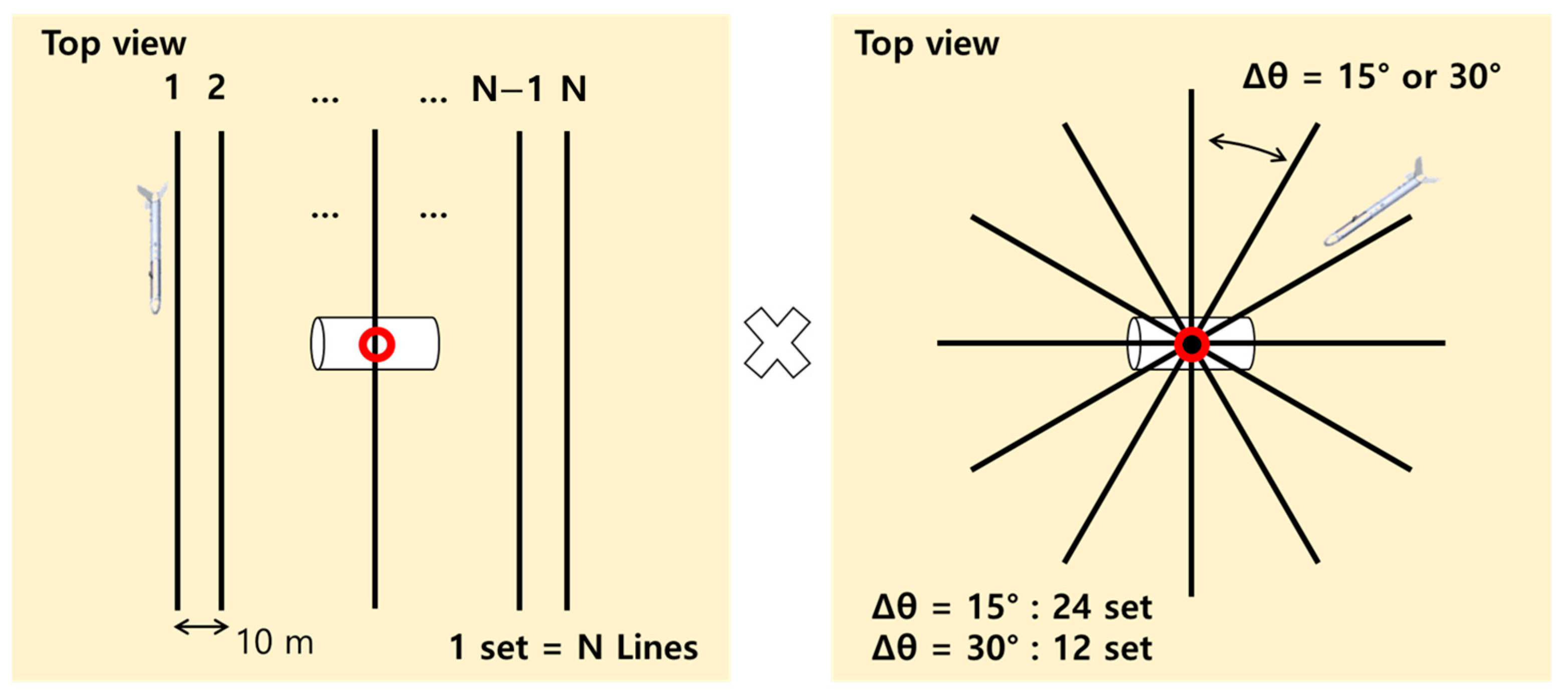
2.1. Sea Experiment

Four sea experiments were conducted to acquire images of seabed targets using side-scan sonar. The SeaView400S sonar system (Figure 1a), manufactured by the Korean company SonarTech (Busan, Republic of Korea), was employed. Its main specifications are described in Kim et al. [15].

Three types of targets were used for image acquisition: manta-shaped targets, open-end cylindrical targets, and closed-end cylindrical targets. In this paper, we analyzed images from closed-end cylindrical targets. These images were acquired in all experiments. They are relatively easy to distinguish from the background. The shape of the closed-end cylindrical target is illustrated in Figure 1b.

The experimental site was divided into two main regions. The sites of experiments 1 and 2 were coastal waters near Geoje, while experiments 3 and 4 were conducted in the waters off the coast of Busan. In the Geoje experiments, the mock-up target was positioned at a depth of approximately 20 m. In the Busan experiments, a mock-up target was placed at a depth of approximately 12 m. A unique aspect of these experiments was the variation in seabed conditions. In experiments 1 and 2, a cylindrical target was placed on a mud area, whereas in experiment 4, the same target was placed on a sand area. For experiment 3, the target was placed on a rock area. However, the data from experiment 3 was excluded from the analysis due to the limited number of samples, as it was difficult to distinguish the target highlight region from the background. Grain size and other details about the experimental site are available in Kim et al. [15]. During our experiments, the mock-up target was not buried in the seabed.

The survey line for side scan sonar image acquisition in the sea experiment is depicted in Figure 2. Depending on the experiment, survey lines were performed at intervals of either 30 degrees or 15 degrees from the target center. Each survey line set consisted of 11 straight-line passes spaced 10 m apart, including one line that directly passed through the target center. This arrangement enabled the acquisition of seabed target images from various angles and distances.

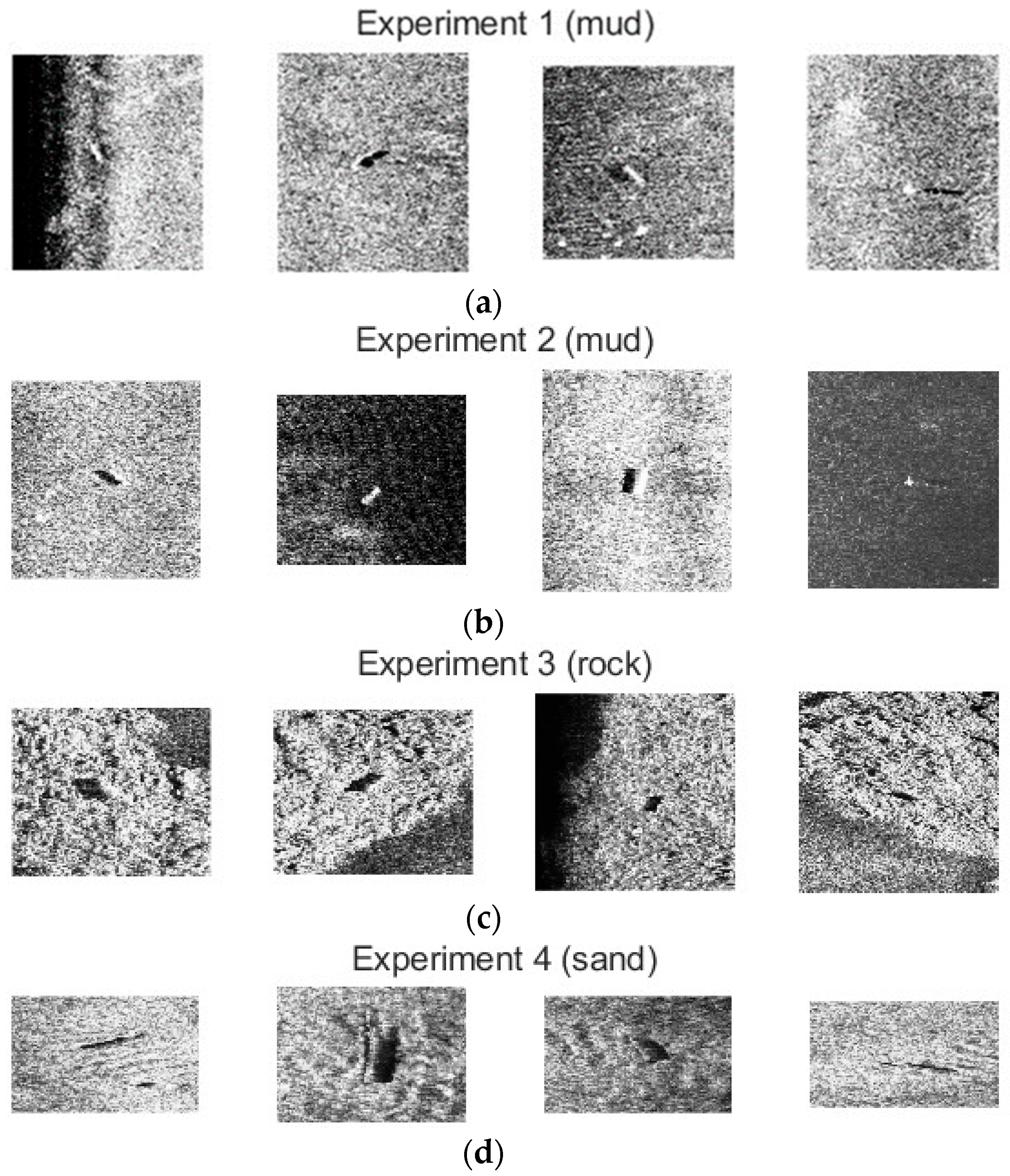
2.2. Target Dataset

As mentioned before, we focused on analyzing closed-ended cylindrical targets in the paper. An example of an image of a cylindrical target obtained through the experiments is shown in Figure 3. These images confirm that the target was captured from various angles. Notably, despite its cylindrical shape, the target appeared similar to a sphere depending on the direction of the survey line.

The dataset revealed that background characteristics near the target and the relative intensity of the target compared to the background varied depending on the experimental sea area. In the mud area (experiments 1 and 2), the target’s presence and its highlight pixels were easily distinguishable. In contrast, distinguishing the target was more challenging in rock (experiment 3) or sand areas (experiment 4).

For the target in the mud area, the intensity contrast between the target highlight and the background generally allowed a clear distinction of the target area, except at certain orientations. Target shadows were identifiable in most cases, except in regions far from the sensor or where background intensity diminished due to the characteristics of the sonar transmission/receive beam pattern. In rock areas, the intensity of rock features was often similar to that of the target highlight, and the highlight and shadow created by the rock terrain resembled the shadow of the target. This similarity made it difficult to identify the target’s presence. In the sand area, the presence of wavy sand dunes near the target led to confusion, as these features resembled the target. While shadows were somewhat easier to distinguish compared to rock areas, the small intensity contrast between the target highlight and the surrounding background area made it difficult to accurately identify target highlight pixels.

As a result, confirming the target presence in rock or sand areas was challenging. Even when the target was detected, we frequently found it challenging to distinguish the highlight pixels from the background pixels near the target. For this study, we analyzed images of cylindrical targets placed in mud area (experiments 1 and 2) and sand area (experiment 4). Regions where the target’s presence was confirmed were cropped to create a dataset for training, validation, and testing. The dataset was constructed using images that included only narrow regions containing target highlights and shadows. The region of each dataset is narrower than the previously described target vicinity area in Figure 3. Extracting narrow areas was necessary to mitigate class imbalance, as pixel frequencies could be otherwise heavily biased toward the background class, hindering effective training. This narrow region can be considered a detection scenario with a tighter bounding box. The dimensions of the cropped images varied, ranging from approximately 20 to 100 pixels, due to differences in the target and shadow shapes depending on the target’s orientation and location.

The dataset size and distribution are presented in

Table 1. The number of the target images in each dataset.

Dataset	Mud	Sand	Experiment	Site
1	209	0	1, 2	Geoje
2	0	174	4	Busan

. The ground truth of labeled pixels for each image in the dataset was manually annotated using the Image Labeler app in MATLAB 2024a.

3. Deep Learning Application Method

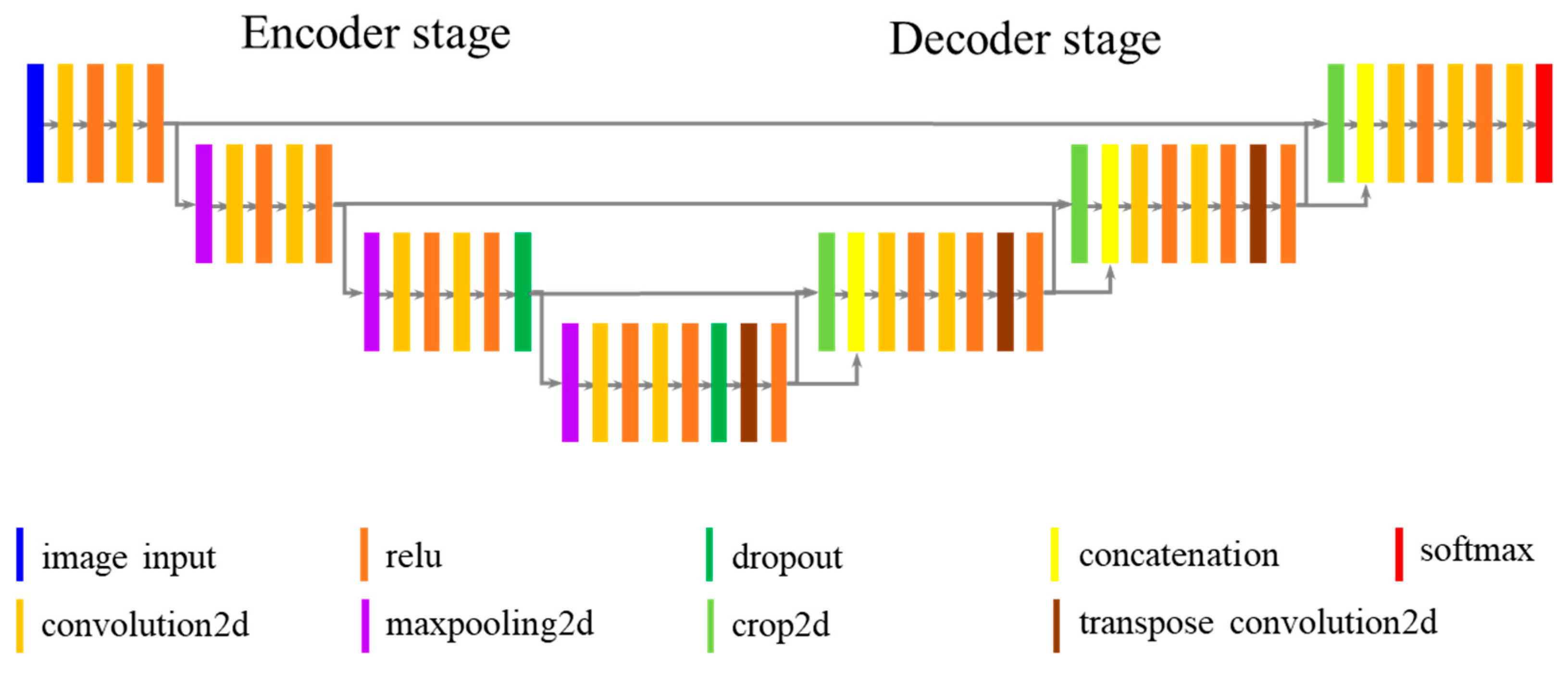
3.1. Network Design

To perform the image segment on the acquired seabed target images, U-NET [27] was employed. U-NET is a neural network architecture originally developed for semantic segmentation in medical imaging. U-NET was selected because of its suitability with a small dataset and its lower complexity compared to competitive algorithms such as PSPNet [28] and Deeplab [29,30]. This method is effective in training on small datasets of approximately 30 images and producing reasonable results. It is also considered suitable for application to larger datasets, such as hundreds of side-scan sonar images collected during sea experiments. Its reliability is further supported by its use as a benchmark in previous studies on semantic segmentation of side-scan sonar images [13,16,17,20].

An example of the U-NET network architecture is illustrated in Figure 4. The network architecture employs an encoder-decoder structure. The encoder compresses input information while the decoder restores the compressed information and assigns a class label to each pixel. Additionally, a skip connection is integrated to utilize compressed information more efficiently during decoding.

Prior to inputting images into U-NET, the image size was resized to 32 × 32 pixels because the image sizes in the datasets differ from one another. In this implementation, the network depth was set to three layers.

3.2. Network Training Options

Cross-entropy loss was used to calculate the loss function of the network. In this paper, we analyzed the situation using two different weighting strategies for loss function. The first was the Equal weight method, which assigns uniform weights to all label classes without accounting for pixel frequency imbalances among label classes. The second method, Pixel-frequency weighting, applies weights based on the inverse of the pixel-frequency ratio to address imbalances in pixel distributions across label classes. The other training parameters were configured with ADAM [31] as the optimization algorithm, 1000 epochs, a mini-batch size of 32, a learning rate of 0.0005, and an L2 regularization coefficient of 0.0001. Data were shuffled at each epoch, and the final trained model was selected based on the epoch that achieved the minimum loss during the validation.

Given the limited size of the dataset, we implemented data augmentation during training, including the addition of background noise and image flipping. Background noise consisted of speckle noise, Gaussian noise, and salt-and-pepper noise. One of three types of noise was applied randomly to each image. The variances for speckle and Gaussian noise were set to 0.05, while salt-and-pepper noise was set to affect 5% of the total area. For image flipping, horizontal (left-right) and vertical (up-down) flips were applied randomly.

The dataset was split into training, validation, and test subsets in a ratio of 6:2:2. The test set was separated first, and k-fold validation (k = 4) was performed on the training-validation data, maintaining a 6:2 ratio for each fold.

For the analysis, the training was performed by CPU only. The CPU specification was 12th Gen Intel(R) Core(TM) i7-12700 (2.10 GHz), and the RAM size is 64 GB. The storage size of the network is around 28 MB. The time for each training process is around 2 h when both datasets are used and trained by the CPU. We can expect that the model can be used in an actual system because the model is quite light, and it takes a short time to process image segmentation using the trained network.

4. Results

In this section, we show the result of the analysis. At first, examples of image segmentation prediction are shown and compared with truth labels and predicted label regions. We describe the performance metrics and qualitatively analyze the two main cases related to the dataset:

• The case where train, validation, and test datasets are the same
  • Weight type of loss function,
  • Seabed type (dataset)
• The case where the dataset of train and validation and the dataset of test are different
  • The network trained on a single dataset only,
  • The network is trained on both datasets.

4.1. The Examples for the Image Segmentation

Before the detailed analysis, the example of image segmentation is shown here. The specifics of the network for the results are as follows: the network is trained on both datasets 1 and 2, and the weight for the loss function is treated equally. The segmentation examples of target highlight and shadow class in the mud area are shown in Figure 5a, and the examples of target highlight and shadow class in the sand area are shown in Figure 5b. The prediction in the mud area seldom showed a little miss and false positive. The prediction in the sand area sometimes makes a large miss in the target highlight class (the image in the 4th row and 3rd column in Figure 5b).

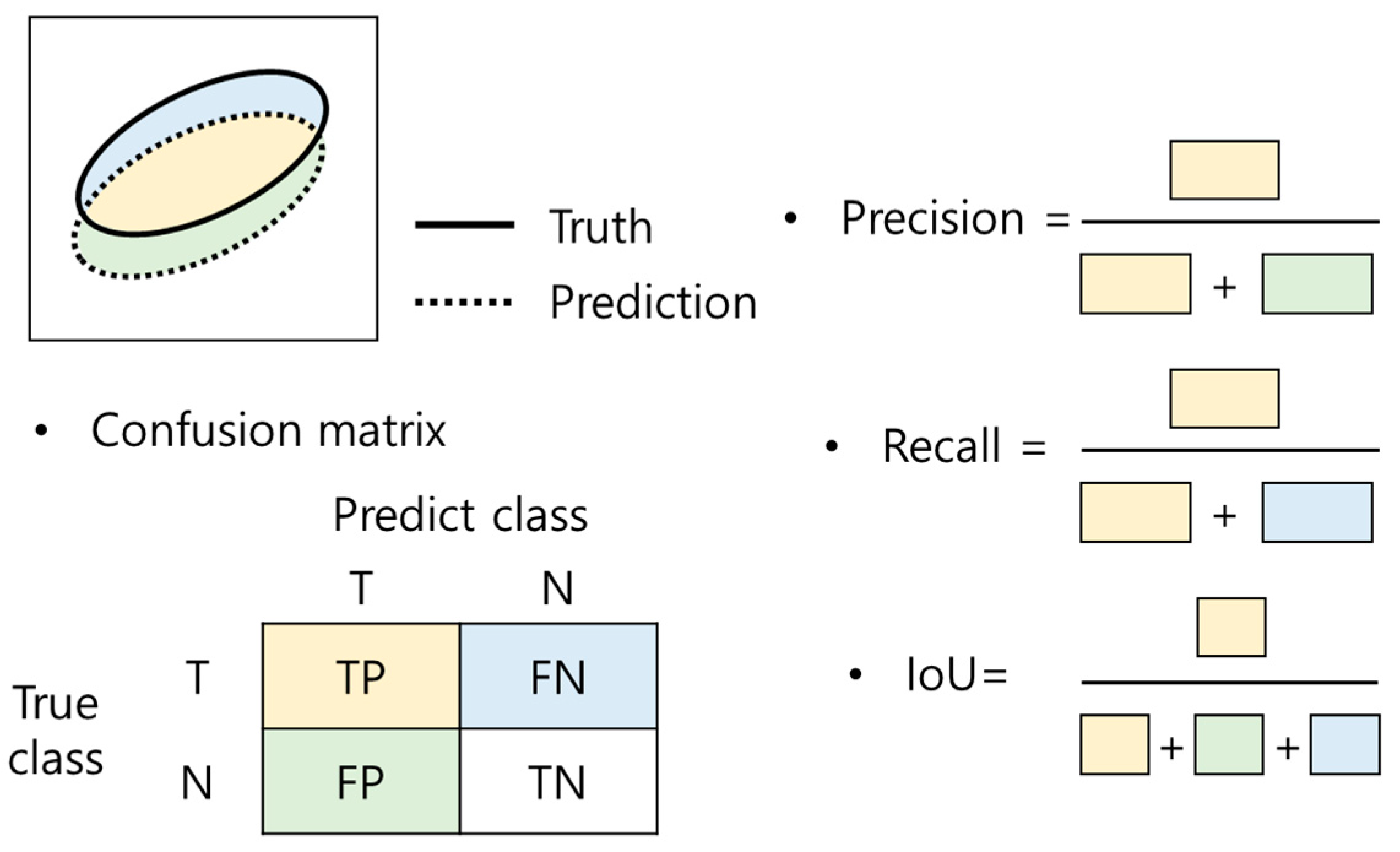
4.2. The Performance Metrics

To evaluate the test results, the following metrics were used: class-specific Precision, class-specific Recall, and class-specific Intersection over Union (IoU). We excluded the Accuracy metric because we deemed it unsuitable for scenarios with significant pixel-frequency imbalances between classes. A conceptual diagram illustrating the metrics is presented in Figure 6.

The confusion matrix shown in Figure 6 compares the predicted values with the actual values for each class label across the entire test dataset. It aggregates the number of pixels correctly identified (True Positives, TP) and the number of pixels incorrectly identified (False Positives, FP) or missed (False Negatives, FN). Based on this matrix, Precision, Recall, and IoU can be calculated.

Precision, Recall and IoU are defined below,

$$\mathrm{Precision}={\displaystyle \frac{\mathrm{T}\mathrm{P}}{\mathrm{T}\mathrm{P}+\mathrm{F}\mathrm{P}}},$$

(1)

$$\mathrm{Recall}={\displaystyle \frac{\mathrm{T}\mathrm{P}}{\mathrm{T}\mathrm{P}+\mathrm{F}\mathrm{N}}},$$

(2)

$$\mathrm{IoU}={\displaystyle \frac{\mathrm{T}\mathrm{P}}{\mathrm{T}\mathrm{P}+\mathrm{F}\mathrm{P}+\mathrm{F}\mathrm{N}}}.$$

(3)

Precision represents the proportion of correctly identified pixels among all predicted positive pixels. The recall represents the proportion of correctly identified pixels among all actual positive pixels. IoU measures the overlap between the actual pixel set and the predicted pixel set, divided by their union. IoU is considered a comprehensive metric as it incorporates both Recall and Precision.

According to these definitions, Precision, Recall, and Io, values closer to 0 indicate poor image segmentation performance, while values approaching 1 signify excellent segmentation performance.

4.3. The Case Where the Datasets of Train, Validation and Test Are the Same

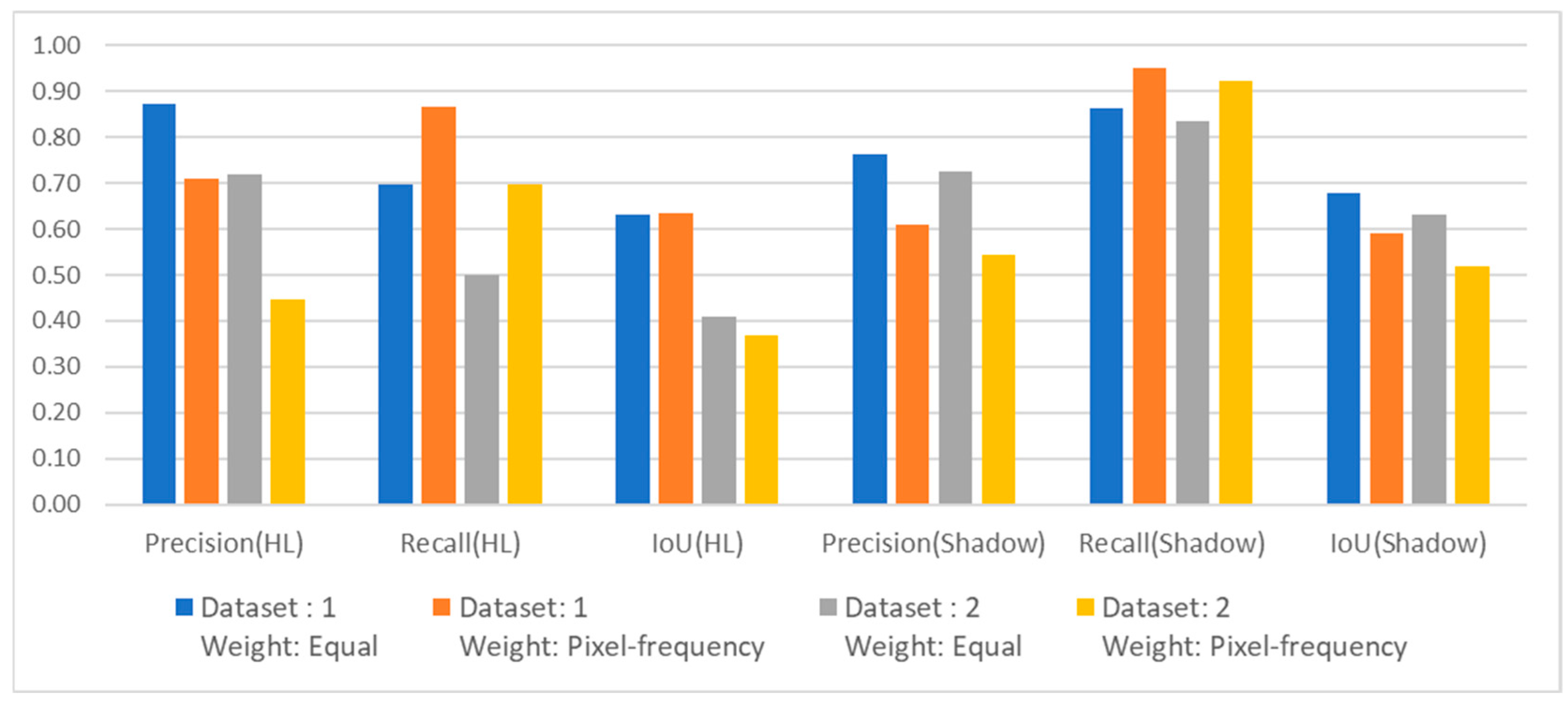
4.3.1. Perspective for the Weight of Loss Function

First, we analyzed the results based on weighting types applied to the cross-entropy loss function. Two weighting strategies were considered: applying equal weights (Equal) and employing class-specific weights based on the inverse of the pixel frequency ratio (Pixel-frequency). For seabed target images, where the pixel frequency of the target class was significantly lower than that of the background, we employed pixel-frequency weighting to address this imbalance.

Figure 7 illustrates the average performance metrics across k-folds. We present each k-fold test result in

Table 2. Segmentation metrics for each k-fold result using dataset 1 (mud area) for training, validation and testing. Different weight types for loss function were applied to analyze their impact.

Specification
Dataset				1
Optimizer				ADAM
Loss function				Cross entropy loss
k-fold	Loss function weight type	HL			Shadow
		Precision	Recall	IoU	Precision	Recall	IoU
1	Equal	0.88	0.70	0.64	0.75	0.87	0.68
2		0.84	0.74	0.65	0.74	0.87	0.67
3		0.90	0.66	0.62	0.76	0.87	0.68
4		0.87	0.68	0.62	0.80	0.83	0.69
Mean		0.87	0.70	0.63	0.76	0.86	0.68
1	Pixel- frequency	0.67	0.90	0.62	0.62	0.96	0.61
2		0.63	0.92	0.60	0.66	0.91	0.62
3		0.75	0.83	0.65	0.57	0.97	0.56
4		0.78	0.81	0.66	0.59	0.97	0.58
Mean		0.71	0.87	0.63	0.61	0.95	0.59

(dataset 1) and

Table 3. Segmentation metrics for each k-fold result using dataset 2 (sand area) for training, validation and testing. Different weight types for loss function were applied to analyze their impact.

Specification
Dataset				2
Optimizer				ADAM
Loss function				Cross entropy loss
k-fold	Loss function weight type	HL			Shadow
		Precision	Recall	IoU	Precision	Recall	IoU
1	Equal	0.77	0.28	0.26	0.71	0.85	0.63
2		0.69	0.56	0.44	0.69	0.86	0.62
3		0.74	0.56	0.46	0.71	0.83	0.62
4		0.68	0.60	0.47	0.78	0.80	0.66
Mean		0.72	0.50	0.41	0.72	0.83	0.63
1	Pixel- frequency	0.56	0.65	0.43	0.51	0.94	0.50
2		0.35	0.75	0.32	0.52	0.92	0.50
3		0.51	0.68	0.41	0.58	0.92	0.55
4		0.36	0.72	0.32	0.57	0.91	0.54
Mean		0.45	0.70	0.37	0.54	0.92	0.52

(dataset 2). Our analysis of both datasets showed the effects of pixel-frequency weighting. Compared to equal weighting, pixel-frequency weighting resulted in lower precision and higher recall for both target highlight and shadow classes. This trend was more pronounced in dataset 2 than in dataset 1. The weighting methods caused significant differences in precision and recall trends. These differences were more pronounced for the highlight area compared to the shadow area. Regarding IoU, dataset 1 exhibited similar IoU values for highlight across weighting methods, whereas dataset 2 case showed improved IoU performance with equal weights. For shadows, superior IoU results were observed for both datasets when equal weights were applied.

Lower precision and higher recall indicate an increase in false positives and a decrease in misses, suggesting that the predicted region of interest is larger than the actual labeled pixel region. If the goal is to minimize false positives during image segmentation, the loss function with equal weights is preferable. Since IoU balances false positives and misses, IoU further supports the effectiveness of using equal weights.

4.3.2. Perspective for the Seabed Type (Dataset)

Next, we analyzed the characteristics of target highlight and target shadow for each seabed type (dataset). We analyzed two cases. The first case used individual datasets for learning. The second case combined both datasets for learning. For this analysis, the loss function weight was set to equal weights based on the result of the previous section.

For the target highlight class, the image segmentation metrics were observed to be superior when using Dataset 1. In the mud area, the target highlight is easier to distinguish from the background than in the sand area. For the target shadow class, the recall consistently achieved a high value of 0.8 or higher across all comparison cases, with both datasets consistently demonstrating higher recall than precision. IoU for shadow was generally better than for highlight (Figure 7). These findings suggest that the neural network performed better in segmenting regions identified as target shadows compared to target highlights.

Additionally, Figure 7 shows that IoU differences between the target highlight and shadow classes were more pronounced in dataset 2 than in dataset 1. This suggests that the sand area (dataset 2) offers a clearer distinction between target shadows and the background. In contrast, the mud area (dataset 1) shows less distinction. Human visual inspection, as shown in Figure 3, supports this observation. This characteristic appears to have been effectively learned by the neural network, contributing to the observed performance trends.

4.4. The Case Where the Dataset of Train and Validation and the Dataset of Test Are Different

In this section, we analyzed the testing results on datasets from seabed types that were different from those used for training and validation. This approach assumes that a neural network is trained on data acquired from a specific sea area. The trained network is then applied to images from other sea areas. For instance, a neural network trained on seabed target images acquired in a sand area is applied to segment seabed target images from a mud area. Performance comparisons were based on the results of the previous analysis. This analysis tested datasets from different sources and those identical to the training and validation datasets. For the network settings, we employed the ADAM optimizer and set the loss function weights to equal weights. The following presents the results of the performance metric comparison based on changes in the dataset. Figure 8 illustrates the average k-fold performance metrics for the target highlight class. Figure 9 presents the corresponding metrics for the target shadow class. Each k-fold result for all cases is shown in

Table 4. Segmentation metrics for each k-fold result are based on the combination of training/validation and test datasets.

Specification
Optimizer				ADAM
Loss function				Cross entropy loss with equal weight
k-fold	Dataset		HL			Shadow
	Training/ Validiation	Test	Precision	Recall	IoU	Precision	Recall	IoU
1	1	1	0.88	0.70	0.64	0.75	0.87	0.68
2			0.84	0.74	0.65	0.74	0.87	0.67
3			0.90	0.66	0.62	0.76	0.87	0.68
4			0.87	0.68	0.62	0.80	0.83	0.69
Mean			0.87	0.70	0.63	0.76	0.86	0.68
1	2	1	0.86	0.55	0.51	0.65	0.80	0.56
2			0.79	0.70	0.59	0.65	0.83	0.57
3			0.81	0.72	0.62	0.66	0.86	0.59
4			0.82	0.71	0.62	0.73	0.79	0.61
Mean			0.82	0.67	0.58	0.67	0.82	0.58
1	1, 2	1	0.87	0.72	0.65	0.75	0.90	0.69
2			0.86	0.72	0.64	0.76	0.86	0.67
3			0.86	0.72	0.65	0.74	0.88	0.67
4			0.89	0.67	0.62	0.82	0.80	0.68
Mean			0.87	0.71	0.64	0.77	0.86	0.68
1	1	2	0.71	0.41	0.35	0.80	0.81	0.67
2			0.57	0.50	0.37	0.76	0.84	0.66
3			0.79	0.33	0.30	0.77	0.82	0.66
4			0.66	0.39	0.32	0.83	0.76	0.66
Mean			0.68	0.41	0.34	0.79	0.81	0.66
1	2	2	0.77	0.28	0.26	0.71	0.85	0.63
2			0.69	0.56	0.44	0.69	0.86	0.62
3			0.74	0.56	0.46	0.71	0.83	0.62
4			0.68	0.60	0.47	0.78	0.80	0.66
Mean			0.72	0.50	0.41	0.72	0.83	0.63
1	1, 2	2	0.74	0.58	0.48	0.74	0.86	0.66
2			0.71	0.57	0.47	0.79	0.85	0.69
3			0.72	0.50	0.42	0.76	0.85	0.67
4			0.81	0.48	0.44	0.82	0.79	0.67
Mean			0.75	0.53	0.45	0.78	0.83	0.67

. Cases where the same dataset was used for training, validation, and testing, were compared simultaneously. In addition, we presented the performance of the network trained using both dataset 1 and dataset 2. This demonstrates the effect of datasets acquired from heterogeneous seabed types on network learning.

4.4.1. Network Trained on Using Single Dataset Only

First, we analyzed the case where dataset 1 was used for training and validation, and dataset 2 was used for testing. In this case, all three metrics related to target highlight showed a decline. Notably, The IoU metric decreased significantly, dropping from 0.63 to 0.34. This reduction occurred compared to the case where the same dataset (dataset 1) was used for testing. This phenomenon can be explained by the intense contrast between the background and the target highlight in images acquired from different seabed types. Specifically, seabed target images from the mud area (dataset 1) exhibit a high contrast between the target highlight intensity and the background intensity. This contrast makes the highlight visually distinguishable. Seabed target images from the sand area (dataset 2) display a small intensity contrast between the background and target highlight. This makes visual inspection by humans more challenging. The trained neural network appears to reflect this characteristic in its predictions. For the target shadow class, the precision performance improved slightly, but recall and IoU showed a minor decline, and their differences were smaller than the observed changes in target highlight metrics.

Next, we analyzed the case where dataset 2 was used for training and validation. For the target highlight class, the testing performance with dataset 1 was superior to that with dataset 2, with significant improvements in recall and IoU. We inferred that training on dataset 2 (sand area) enhances the generalization capability of image segmentation. Segmenting the target highlight class in the sand area is challenging. These conditions enable the network to learn deeper features of the target highlight class. Consequently, the network’s segmentation performance improves for images from the mud area. This is because the distinction between the background and highlight is more pronounced in the mud area. For the target shadow class, all three metrics performed better when dataset 2 was used for testing. However, the performance increase for the target shadow class was smaller. It did not show as significant changes as those observed in recall and IoU for the target highlight class.

4.4.2. Network Trained on Using Dataset 1 and Dataset 2 Both

When the network was trained and validated using both Datasets 1 and 2, the test results for each dataset outperformed those of networks trained and validated on a single dataset.

For the target highlight class, testing on Dataset 1 showed slight improvements in recall and IoU compared to networks trained on individual datasets, while testing on Dataset 2 showed improvements across all three metrics. For the target shadow class, testing on Dataset 1 achieved performance comparable to the network trained on Dataset 1 and superior to the network trained on Dataset 2. Testing on Dataset 2 showed moderate precision and recall, falling between the metrics obtained from testing on each individual dataset, while IoU showed a slight improvement compared to networks trained on a single dataset.

These results suggest that the generalized ability to detect features of target highlight was enhanced by learning highlight shapes across various seabed conditions. This finding indicates that incorporating datasets acquired from various seabed environments can contribute to the improvement of image segmentation performance.

5. Conclusions

We investigated the effect of seabed types on segmentation performance using a deep learning-based approach. Specifically, we analyzed images of the cylindrical target overlying two distinct seabed types: mud and sand. The datasets collected during sea experiments on the coast of South Korea were categorized based on seabed type. For image segmentation, we utilized the U-NET architecture with three label classes: target highlight, target shadow, and background.

In summary, we draw the following conclusions:

• When the training, validation, and test datasets are the same, comparing the loss function’s weight type, the segmentation metrics using equal weight are better than weight considering pixel frequency. This improvement is indicated by the IoU for the highlight class in dataset 2 (0.41 compared to 0.37).
• When the training, validation, and test datasets are the same, the segmentation performance for the target highlight class and shadow class is superior when using only the mud area dataset compared to using only the sand area dataset. This difference is indicated by the IoU for the highlight class (0.63 compared to 0.41) and the IoU for the shadow class (0.68 compared to 0.63). Hence, the target in the mud area is easier to distinguish from the bottom compared to the target in the sand area.
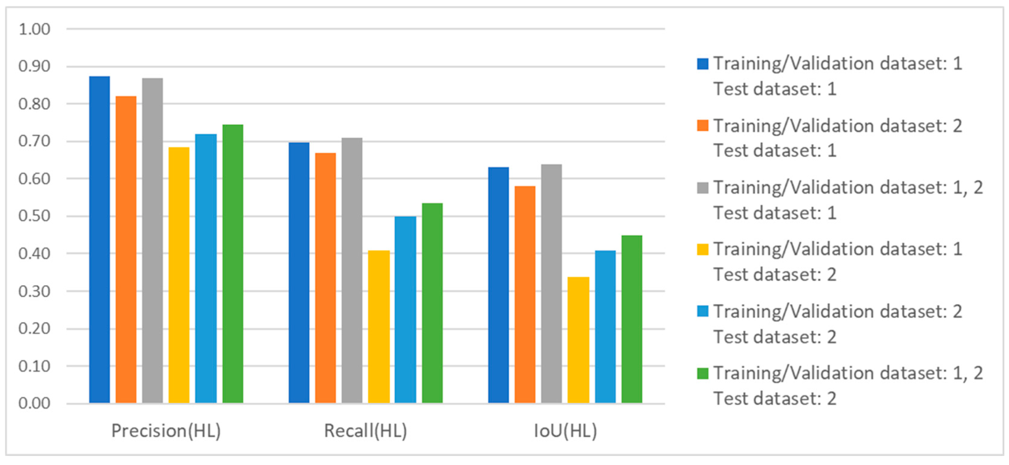
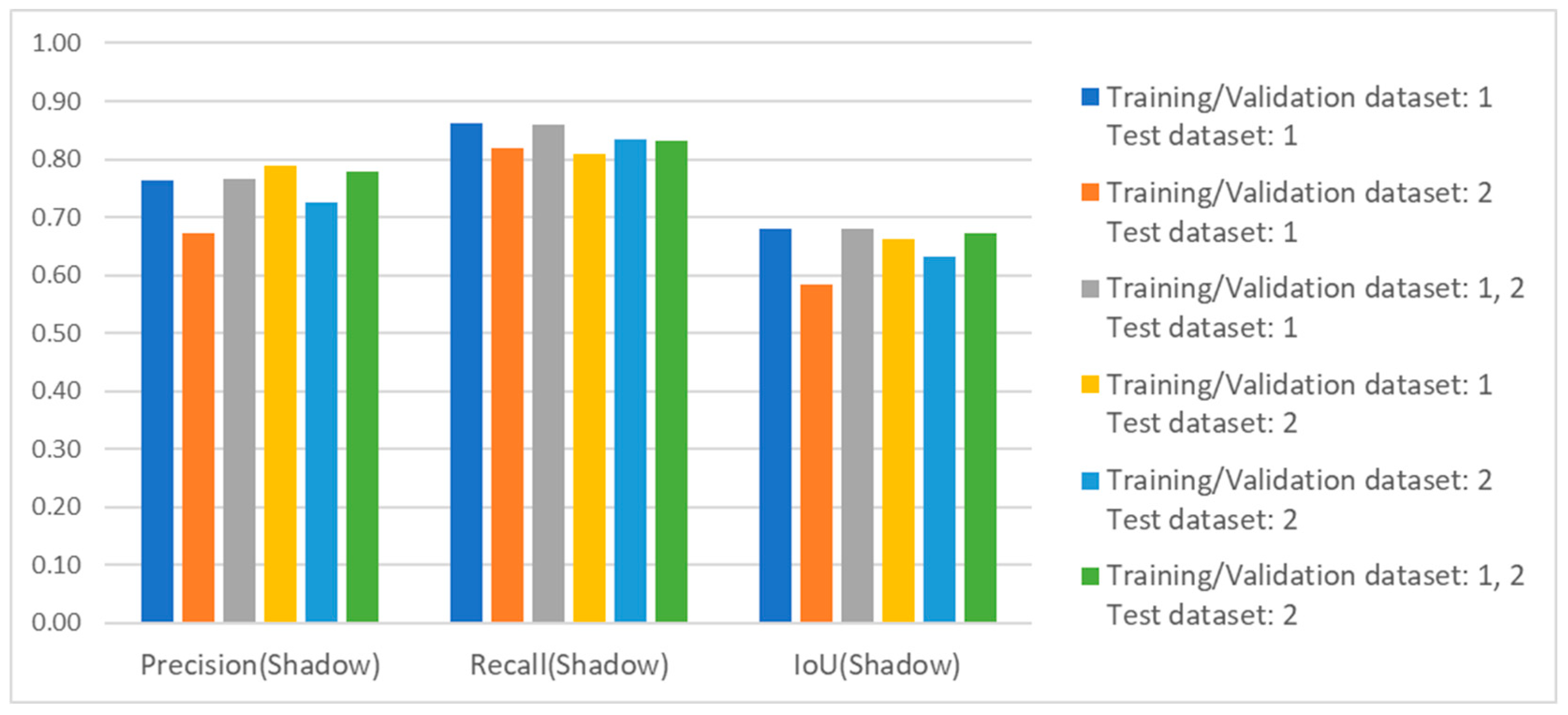
• When the network is trained and validated on mud area data, the image segmentation performance for the target shadow class was consistent across the mud and sand test dataset. This is indicated by the IoU values: 0.68 in the mud area and 0.66 in the sand area. However, the performance of the target highlight class dropped significantly in the sand test data compared to the mud test data. The IoU values indicate this difference: 0.63 in the mud area and 0.34 in the sand area.
• When the network was trained and validated on sand area data, the image segmentation performance for the target shadow class on mud test data decreased slightly. This is indicated by the IoU values: 0.58 in the mud area and 0.63 in the sand area. However, the performance of the target highlight class dropped significantly in the sand test data compared to the mud test data. The IoU values indicate this difference: 0.58 in the mud area and 0.41 in the sand area.
• The performance of the network training and validation using datasets obtained from both sand and mud areas was improved. When testing on the mud area dataset, no significant difference in performance was observed. However, when testing on the sand area dataset, we noted improved image segmentation performance for the target highlight class and shadow class compared to using only every single dataset throughout the training, validation, and test processes. The IoU values for the highlight class in sand area images are as follows: 0.34 for training on mud, 0.41 for training on sand, and 0.45 for training on both.

Hence, we conclude that the target images from various seabeds are needed to improve the image segmentation performance of the target using side scan sonar. The trend of the performance metrics may vary depending on the source of the dataset, such as the sea experiment site. These variations are also expected when image segmentation is applied to data from sea areas with the same seabed type but different grain size properties.

For future work, we plan to enhance the network design for image segmentation and improve the network’s applicability to real-world systems, such as AUVs. If feasible, we will conduct additional sea experiments using side-scan sonar to expand the dataset of target images overlying diverse seabed types.

References

- Stewart, W.I.; Chu, D.; Malik, S.; Lerner, S.; Singh, H. Quantitative seafloor characterization using a bathymetric sidescan sonar. IEEE J. Ocean. Eng. 1994, 19, 599–610. [Google Scholar] [CrossRef]
- Iacono, C.L.; Gràcia, E.; Diez, S.; Bozzano, G.; Moreno, X.; Dañobeitia, J.; Alonso, B. Seafloor characterization and backscatter variability of the Almería Margin (Alboran Sea, SW Mediterranean) based on high-resolution acoustic data. Mar. Geol. 2008, 250, 1–18. [Google Scholar] [CrossRef]
- Yang, D.; Wang, C.; Cheng, C.; Pan, G.; Zhang, F. Semantic segmentation of side-scan sonar images with few samples. Electronics 2022, 11, 3002. [Google Scholar] [CrossRef]
- Burguera, A.; Bonin-Font, F. On-line multi-class segmentation of side-scan sonar imagery using an autonomous underwater vehicle. J. Mar. Sci. Eng. 2020, 8, 557. [Google Scholar] [CrossRef]
- Yan, J.; Meng, J.; Zhao, J. Real-time bottom tracking using side scan sonar data through one-dimensional convolutional neural networks. Remote Sens. 2019, 12, 37. [Google Scholar] [CrossRef]
- Yan, J.; Meng, J.; Zhao, J. Bottom detection from backscatter data of conventional side scan sonars through 1D-UNet. Remote Sens. 2021, 13, 1024. [Google Scholar] [CrossRef]
- Mignotte, M.; Collet, C.; Perez, P.; Bouthemy, P. Sonar image segmentation using an unsupervised hierarchical MRF model. IEEE Trans. Image Process. 2000, 9, 1216–1231. [Google Scholar] [CrossRef]
- Acosta, G.G.; Villar, S.A. Accumulated CA–CFAR process in 2-D for online object detection from sidescan sonar data. IEEE J. Ocean. Eng. 2015, 40, 558–569. [Google Scholar] [CrossRef]
- Tueller, P.; Kastner, R.; Diamant, R. A comparison of feature detectors for underwater sonar imagery. In Proceedings of the OCEANS 2018 MTS/IEEE Charleston, Charleston, SC, USA, 22–25 October 2018; pp. 1–6. [Google Scholar] [CrossRef]
- Wang, X.; Wang, L.; Li, G.; Xie, X. A robust and fast method for sidescan sonar image segmentation based on region growing. Sensors 2021, 21, 6960. [Google Scholar] [CrossRef]
- Gebhardt, D.; Parikh, K.; Dzieciuch, I.; Walton, M.; Vo Hoang, N.A. Hunting for naval mines with deep neural networks. In Proceedings of the OCEANS 2017—Anchorage, Anchorage, AK, USA, 18–21 September 2017; pp. 1–5. [Google Scholar]
- Kim, J.; Choi, J.W.; Kwon, H.; Oh, R.; Son, S.-U. The application of convolutional neural networks for automatic detection of underwater objects in side-scan sonar images. J. Acoust. Soc. Kor 2018, 37, 118–128. [Google Scholar] [CrossRef]
- Wu, M.; Wang, Q.; Rigall, E.; Li, K.; Zhu, W.; He, B.; Yan, T. ECNet: Efficient convolutional networks for side scan sonar image segmentation. Sensors 2019, 19, 2009. [Google Scholar] [CrossRef] [PubMed]
- Thanh Le, H.; Phung, S.L.; Chapple, P.B.; Bouzerdoum, A.; Ritz, C.H.; Tran, L.C. Deep gabor neural network for automatic detection of mine-like objects in sonar imagery. IEEE Access 2020, 8, 94126–94139. [Google Scholar] [CrossRef]
- Kim, W.K.; Bae, H.S.; Son, S.U.; Park, J.S. Neural network-based underwater object detection off the coast of the Korean Peninsula. J. Mar. Sci. Eng. 2022, 10, 1436. [Google Scholar] [CrossRef]
- Wang, Z.; Guo, J.; Huang, W.; Zhang, S. Side-scan sonar image segmentation based on multi-channel fusion convolution neural networks. IEEE Sens. J. 2022, 22, 5911–5928. [Google Scholar] [CrossRef]
- Shi, P.; Sun, H.; He, Q.; Wang, H.; Fan, X.; Xin, Y. An effective strategy of object instance segmentation in sonar images. IET Signal Process. 2024, 2024, 1357293. [Google Scholar] [CrossRef]
- Wang, W.; Zhang, Y.; Li, H.; Kang, Y.; Liu, L.; Chen, C.; Zhai, G. A novel target detection method with dual-domain multi-frequency feature in side-scan sonar images. IET Image Process. 2024, 18, 4168–4188. [Google Scholar] [CrossRef]
- Wen, X.; Wang, J.; Cheng, C.; Zhang, F.; Pan, G. Underwater side-scan sonar target detection: YOLOv7 model combined with attention mechanism and scaling factor. Remote Sens. 2024, 16, 2492. [Google Scholar] [CrossRef]
- Sun, Y.; Zheng, H.; Zhang, G.; Ren, J.; Shu, G. CGF-Unet: Semantic segmentation of sidescan sonar based on UNET combined with global features. IEEE J. Ocean. Eng. 2024, 49, 8346–8360. [Google Scholar] [CrossRef]
- Zhu, J.; Cai, W.; Zhang, M.; Pan, M. Sonar image coarse-to-fine few-shot segmentation based on object-shadow feature pair localization and level set method. IEEE Sens. J. 2024, 24, 8346–8360. [Google Scholar] [CrossRef]
- Huo, G.; Wu, Z.; Li, J. Underwater object classification in sidescan sonar images using deep transfer learning and semisynthetic training data. IEEE Access 2020, 8, 47407–47418. [Google Scholar] [CrossRef]
- Zhang, P.; Tang, J.; Zhong, H.; Ning, M.; Liu, D.; Wu, K. Self-trained target detection of radar and sonar images using automatic deep learning. IEEE Trans. Geosci. Remote Sens. 2022, 60, 4701914. [Google Scholar] [CrossRef]
- Santos, N.P.; Moura, R.; Torgal, G.S.; Lobo, V.; de Castro Neto, M. Side-scan sonar imaging data of underwater vehicles for mine detection. Data Brief 2024, 53, 110132. [Google Scholar] [CrossRef] [PubMed]
- Talukdar, K.K.; Tyce, R.C.; Clay, C.S. Interpretation of Sea Beam backscatter data collected at the Laurentian fan off Nova Scotia using acoustic backscatter theory. J. Acoust. Soc. Am. 1995, 97, 1545–1558. [Google Scholar] [CrossRef]
- Chotiros, N.P. Seafloor acoustic backscattering strength and properties from published data. In Proceedings of the OCEANS 2006—Asia Pacific, Singapore, 16–19 May 2006; pp. 1–6. [Google Scholar] [CrossRef]
- Ronneberger, O.; Fischer, P.; Brox, T. U-Net: Convolutional networks for biomedical image segmentation. In Proceedings of the Medical Image Computing and Computer-Assisted Intervention—MICCAI 2015, Munich, Germany, 5–9 October 2015; pp. 234–241. [Google Scholar] [CrossRef]
- Zhao, H.; Shi, J.; Qi, X.; Wang, X.; Jia, J. Pyramid scene parsing network. In Proceedings of the IEEE Conference on Computer Vision and Pattern Recognition, Honolulu, HI, USA, 21–26 July 2017; pp. 2881–2890. [Google Scholar] [CrossRef]
- Chen, L.-C.; Papandreou, G.; Kokkinos, I.; Murphy, K.; Yuille, A.L. Semantic image segmentation with deep convolutional nets and fully connected CRFs. arXiv 2014, arXiv:1412.7062. [Google Scholar] [CrossRef]
- Chen, L.-C.; Papandreou, G.; Schroff, F.; Adam, H. Rethinking atrous convolution for semantic image segmentation. arXiv 2017, arXiv:1706.05587. [Google Scholar] [CrossRef]
- Kingma, D.; Ba, J. Adam: A method for stochastic optimization. arXiv 2017, arXiv:1412.6980. [Google Scholar] [CrossRef]