Abstract
Sea surface wind speed is a crucial parameter for studying climate change and ocean dynamics. Accurate, real-time measurements are essential for meteorological and oceanographic observations. Global Navigation Satellite System Reflectometry (GNSS-R) is a key technology for sea surface wind speed retrieval. Existing wind speed retrieval models employ two primary approaches: unified modeling across the entire wind speed range and independent modeling for partitioned wind speed intervals. The former cannot effectively address physical property variations across wind speed ranges. The latter, while mitigating this issue, relies on empirical thresholds for interval partitioning that ignore actual data distribution and struggles to assign new samples to appropriate intervals during prediction. To address these limitations, this study employs the Gradient-Boosted Adaptive Multi-Objective Simulated Annealing (GAMSA) algorithm to construct a multi-objective optimization function and perform data-driven wind speed interval partitioning. Specialized XGBoost sub-models are then constructed for each partitioned interval, and their predictions are integrated through a stacking ensemble learning architecture. The experiments utilize a Cyclone Global Navigation Satellite System (CYGNSS) and ERA5 reanalysis data. The experimental results show that the proposed method reduces the root mean square error (RMSE) from 1.77 m/s to 1.43 m/s and increases the coefficient of determination (R2) from 0.6293 to 0.7770 compared with a global XGBoost model. It also exhibits enhanced accuracy under high wind speeds (>16 m/s) and, when independently validated with buoy data, achieves an RMSE of 1.52 m/s and R2 of 0.79. The proposed method improves retrieval accuracy across both overall and individual wind speed intervals, avoids the sample isolation problem inherent in traditional empirical partitioning methods, and resolves the issue of assigning new samples to appropriate sub-models during application.
1. Introduction
Sea surface wind speed, a key parameter in ocean–atmosphere interactions [1,2], plays a crucial role in understanding ocean climate systems, ensuring maritime navigation safety, and monitoring and forecasting marine disasters [3,4]. Traditional sea surface wind speed observations primarily rely on marine meteorological stations [5], buoys [6], and meteorological satellites [7,8], which provide high-precision wind field data but have significant limitations. Marine meteorological stations and buoys are deployed at fixed locations with high installation and maintenance costs, making large-scale deployment difficult and resulting in insufficient coverage of vast ocean areas [9]. Although traditional meteorological satellites possess large-scale observation capabilities, their long revisit periods limit temporal continuity [10].
In the 1990s, Martín-Neira [11] first proposed using GPS reflected signals for sea surface height measurement, initiating research on satellite-reflected signal Earth observation. Zavorotny and Voronovich [12] established a theoretical framework linking reflected GPS signals to sea surface roughness in 2000, confirming that the power and waveform characteristics of reflected signals can infer sea surface wind speed, thereby laying the theoretical foundation for subsequent wind speed retrieval research. With continuous advancement, Global Navigation Satellite System Reflectometry (GNSS-R) technology has been progressively refined and has become an important tool for global sea surface wind speed monitoring [13], owing to its advantages of abundant signal sources, all-weather capability, low cost, and high coverage [14,15,16]. Early GNSS-R wind speed retrieval primarily relied on the Geophysical Model Function (GMF) approach. Clarizia et al. [17] proposed the Minimum Variance Estimator (MVE) method based on Delay-Doppler Maps (DDMs) in 2014, which improved wind speed retrieval accuracy by extracting features such as normalized bistatic radar cross-section (NBRCS) and leading-edge slope (LES) [18]. However, the GMF method has relatively simple parameter settings, mainly considering wind speed-related observables and incidence angles, making it difficult to fully capture the complex nonlinear relationships between sea surface scattering characteristics and signal responses under different sea conditions [19]. To overcome these limitations, researchers have recently applied machine learning techniques to GNSS-R wind speed retrieval, leveraging their powerful nonlinear fitting capabilities to enhance retrieval accuracy [20,21]. Reynolds et al. [22] employed Artificial Neural Networks (ANNs) to introduce additional observables, such as specular point latitude and longitude and receiver gain correction (RCG) as feature inputs, improving retrieval accuracy. The CyGNSSnet model proposed by Asgarimehr et al. [23] uses Convolutional Neural Networks to extract features from DDMs, while the FSNet model proposed by Chen et al. [24] combines spatial and frequency domain features to enhance the representation capability for complex sea.
Although the aforementioned methods have continuously innovated at the algorithmic level, they generally employ a single model to fit the relationship between observables and wind speed across the entire wind speed range. Existing studies have shown that GNSS-R data exhibit significant differences in physical characteristics and sample distributions across different wind speed intervals, and a single model struggles to simultaneously adapt to low- and high-wind-speed conditions, resulting in substantial accuracy degradation at high wind speeds [25,26]. To address this issue, researchers have explored interval partitioning modeling strategies. Xue and Sun [27] used an empirical threshold of 10 m/s to partition data and separately trained GBDT models, improving model fitting capabilities in respective wind speed intervals. Wang et al. [28] demonstrated significant differences in optimal algorithms across different wind speed intervals and divided wind speeds at 15 m/s for separate retrieval, achieving improved accuracy in the respective intervals. However, these interval partitioning methods primarily rely on fixed empirical thresholds. Such manually defined partitioning strategies are independent of actual data distribution characteristics and model prediction errors, lacking scientific justification. Moreover, during actual retrieval, the true wind speed of samples is unknown, making it difficult to determine their corresponding wind speed interval and accurately match the appropriate sub-model, which constrains the practical applicability of these methods.
To address these deficiencies, this study proposes the following methodology:
- An interval partitioning strategy based on the Gradient-Boosted Adaptive Multi-Objective Simulated Annealing (GAMSA) algorithm is designed. A multi-objective optimization function is established that simultaneously considers four key factors: overall prediction accuracy, number of partitioned intervals, sample distribution balance, and minimum sample requirements for model training. By integrating the local refinement capability of gradient boosting with the global search capability of simulated annealing, interval partitioning that conforms to the underlying data distribution characteristics is effectively achieved.
- Based on adaptive interval partitioning, retrieval models using Extreme Gradient Boosting (XGBoost) are constructed for each interval, and a Stacking Ensemble (SE) architecture integrates the predictions of multiple interval models, enabling unified retrieval across the entire wind speed range.
The remainder of this paper is organized as follows: Section 2 introduces data sources and processing methods; Section 3 elaborates on the GNSS-R sea surface wind speed retrieval method based on adaptive wind speed interval partitioning and multi-model ensemble, including wind speed interval partitioning using the GAMSA algorithm, establishment of the stacking ensemble learning model, and experimental validation methods; Section 4 analyzes and compares retrieval accuracy across different partitioning methods and validates against advanced deep learning methods and buoy observations; and Section 5 presents the conclusions.
2. Data and Study Area
The datasets used in this study included the CYGNSS dataset, the Fifth-Generation European Centre for Medium-Range Weather Forecasts Reanalysis (ERA5) dataset, and buoy observations from the National Data Buoy Center (NDBC). Data from January to October 2024, November to December 2024, and January to February 2025 were used for model training, parameter optimization, and performance testing, respectively.
2.1. CYGNSS Data
CYGNSS is an eight-satellite low-Earth-orbit constellation launched by NASA in 2016 [29,30] that retrieves ocean parameters, such as sea surface wind speed, by receiving GPS signals reflected from the sea surface, covering tropical cyclone active regions between 38° N and 38° S [31,32]. The geometry of these reflected signal paths is schematically shown in Figure 1. Its Level 1 data contain Earth observation parameters, such as specular point coordinates and antenna gain, satellite operational status indicators, and DDM-related information, from which wind speed retrieval observables such as NBRCS and LES can be extracted [33,34]. This study utilized the CYGNSS Level 1 data variables shown in Table 1.
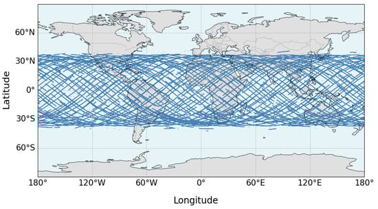
Figure 1.
Schematic diagram of CYGNSS specular point trajectories.

Table 1.
List of input variables used in wind speed retrieval.
To ensure data accuracy and reliability, the following quality control measures were applied: removal of observation samples with missing NBRCS and LES values; exclusion of samples with negative LES values; filtering out samples located in land areas; exclusion of samples with an sp_inc_angle greater than 60° [35,36]; removal of samples with an sp_rx_gain lower than 0; calculation of the receiver gain correction (RCG) for each sample; and removal of samples with RCG values less than 10 [37,38]. The RCG calculation formula is as follows:
where represents the distance from the transmitter to the specular point, represents the distance from the receiver to the specular point, and represents the receiver antenna gain at the specular point.
2.2. ERA5 Data
The reference wind speed data are sourced from ERA5, provided by the European Centre for Medium-Range Weather Forecasts (ECMWF), which contains hourly global sea surface wind speed data since 1979. This dataset generates high-precision wind speed information by integrating extensive historical observations and utilizing an assimilation system, and is widely used as reference meteorological data in remote-sensing research. Its spatial resolution is 0.25° × 0.25°, and its temporal resolution is 1 h, effectively supporting sea surface wind speed retrieval research [39,40]. In this study, the eastward and northward components of the 10 m sea surface wind speed from ERA5 were used to calculate the wind speed at different locations by computing the square root of the sum of squares of these two components [41].
Due to differences in temporal and spatial resolution between ERA5 and CYGNSS data, this study employed a spatiotemporal nearest neighbor matching method to ensure precise alignment [42]. Using ERA5 data as the baseline, CYGNSS observation points nearest to each ERA5 grid center within 5 min were matched with ERA5 reference wind speed data to form individual samples, which collectively constituted the dataset. In comparative experiments with other deep learning methods, identical data sources and consistent data preprocessing and dataset construction methods were used to ensure fair comparison.
2.3. NDBC Buoy Validation Data
To further validate the accuracy and practicality of the proposed method, buoy observations from NDBC were introduced as an independent validation data source. NDBC has deployed numerous ocean observation buoys worldwide, providing high-quality in situ sea surface wind speed observations, including wind speed and direction measurements at a 10 m height with a temporal resolution of 1 h and measurement accuracy of 0.1 m/s [43].
3. Methodology
3.1. Overall Framework of GAMSA-XGB-SE Model
The overall framework of the proposed Gradient-Enhanced Adaptive Multi-Objective Simulated Annealing–XGBoost–Stacking Ensemble (GAMSA-XGB-SE) model is illustrated in Figure 2.
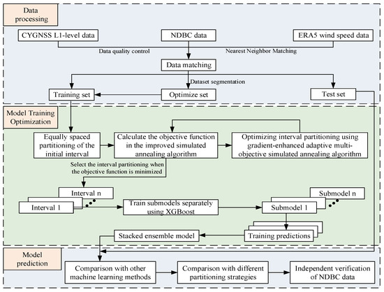
Figure 2.
Flowchart of the experimental procedure.
First, quality control is performed on CYGNSS L1 data to extract key observables such as NBRCS and LES, which are then spatiotemporally matched with ERA5 reanalysis data to construct the dataset. Second, the GAMSA algorithm is employed for adaptive wind speed interval partitioning. Based on the optimal partitioning results, specialized XGBoost prediction models are constructed for each wind speed interval, fully utilizing the data characteristics of different wind speed ranges. Finally, a stacking ensemble learning architecture integrates the predictions from each interval model through a second-level meta-learner, effectively resolving the challenge of assigning new samples to appropriate intervals during prediction and significantly enhancing overall retrieval accuracy.
3.2. Adaptive Wind Speed Interval Partitioning Using the GAMSA Algorithm
This section employs the GAMSA method to construct a multi-objective optimization function that integrates multiple key components, including a fixed normalization strategy, adaptive weight adjustment, and gradient optimization, forming a complete optimization framework.
3.2.1. Multi-Objective Function Design
To achieve optimal wind speed interval partitioning, this study designs an objective function that combines multiple factors. This objective function simultaneously considers four key factors: the model’s overall prediction accuracy, the number of partitioned intervals, the sample distribution, and the minimum sample requirements for model training. Through normalization processing and an adaptive weight adjustment mechanism, it calculates the global optimal solution. The objective function is expressed as
where , , , and represent the normalized sum of prediction errors across intervals, the interval quantity penalty term, the sample distribution variance penalty term, and the minimum sample penalty term, respectively; , , , and represent the corresponding weight coefficients. The settings of weight coefficients , , , and directly influence the relative importance of each optimization objective in the objective function.
The initial values of the weight coefficients are determined through grid search experiments. First, single-factor sensitivity analysis experiments are conducted on each weight coefficient. By independently adjusting each weight within a relatively wide range and observing the convergence of the objective function, the grid search range is determined as , , , and .
On a 20% subset of the training dataset, grid search testing is performed on different weight combinations within this range to determine the initial values of each weight coefficient as , , , and .
To adapt to dynamic changes during the optimization process, the weight coefficients are adaptively adjusted during iteration based on optimization progress. The adjustment strategy is based on the interval change rate and the sample distribution characteristics:
where represents the interval variation rate at the -th iteration:
where and represent the number of intervals in the current and previous iterations, respectively; and are adjustment coefficients for the number of intervals and sample distribution variance, with their values determined experimentally as 0.15 and 0.20, respectively.
Since the prediction error weight serves as the core optimization objective, and the minimum sample requirement weight serves as the fundamental constraint for model validity, their importance should remain stable throughout the optimization process; therefore, they remain constant during optimization. The weight for the number of partitioned intervals is dynamically adjusted based on the interval variation rate—when the number of intervals changes frequently, this weight is increased to stabilize the interval structure. The weight for the sample distribution is adjusted according to the degree of sample distribution imbalance. When the sample distribution is severely uneven, this weight is increased to promote balanced distribution. This adaptive weight adjustment mechanism enables the algorithm to improve optimization effectiveness and convergence speed according to the actual characteristics of the dataset.
The total error term in the objective function represents the sum of prediction errors across all intervals, reflecting the prediction accuracy of each interval. When interval partitioning is appropriate, the error in each interval decreases, and the overall error is reduced. Its calculation formula is
where represents the mean square error of the -th interval, and represents the error weight of the -th interval, which is dynamically calculated based on the interval average wind speed :
where is the base value for error weight calculation. Since the weight should increase with wind speed, the weight value at the lowest wind speed is set as the base value , is the error weight growth coefficient that controls the magnitude of error weight increase with wind speed, and and represent the maximum and minimum wind speeds of the interval, respectively. Due to the scarcity of samples in high-wind-speed intervals and the complexity of sea surface scattering characteristics, prediction is more difficult; thus, higher error weights are assigned.
The interval number penalty term employs an improved penalty function, characterized by generating slight variations even within the target interval range, guiding the algorithm to converge toward the optimal number of intervals, expressed as
where represents the number of intervals, and and represent the target lower and upper limits of the number of intervals, respectively.
The sample distribution variance penalty term quantifies the degree of imbalance in sample distribution across intervals, promoting balanced sample distribution among intervals, expressed as
where and represent the number of samples in the interval and the average number of samples per interval, respectively.
The minimum sample penalty term dynamically constrains intervals with insufficient sample size, addressing model overfitting and interval data distribution estimation bias caused by too few samples, expressed as
where is an indicator function, and represents the dynamic minimum sample requirement for the -th interval, expressed as
where represents the maximum sample requirement, indicating the sample size of the interval with the most sufficient samples, serving as the baseline for setting dynamic minimum sample thresholds. By multiplying by the decay factor , differentiated minimum sample requirements can be set for different wind speed intervals according to their average wind speeds . This design considers the objective differences in the sample distribution across different wind speed intervals. For low-wind-speed intervals with sufficient samples, since is small, the decay term approaches one, and the dynamic minimum sample requirement approaches , imposing stricter sample quantity requirements to ensure model quality. For high-wind-speed intervals with scarce samples, a larger leads to a significant reduction in the decay term, thereby appropriately lowering the minimum sample requirement, ensuring the feasibility and flexibility of the algorithm.
3.2.2. Complete Process of the GAMSA Algorithm
Based on the above objective function and weight settings, the weight coefficients are initialized: , , , and . The interval boundary variables are initialized, the current interval boundary is set to the initial empirical partitioning, and the optimal solution is initially set to as the starting state of the optimization process.
To ensure that each objective term can effectively influence the total function result during the optimization process, this paper adopts a fixed normalization strategy. Before optimization begins, the fixed normalization range of the objective function is determined through initialization sampling:
where is the total error term range, is the interval penalty term range, is the sample variance range, and is the minimum sample penalty term range. The fixed range is determined by collecting statistical information of each factor through multiple random perturbations of the initial interval , with the following expression:
where represents the observed value of the -th factor during the sampling process, and represents the observation span of the -th factor, expressed as
After normalization processing, each component of the objective function is mapped to the same numerical range, ensuring that each factor can exert an appropriate influence during the optimization process.
The main optimization loop of the algorithm continuously refines the interval partitioning scheme through iterative search. In each iteration , a probability , determined empirically to optimally balance search diversity and convergence stability, is used to decide whether to adjust the number of intervals or perturb the boundaries, generating new candidate interval boundaries, as shown in the following formula:
where is the perturbation intensity related to temperature, calculated as
After generating the candidate solution, its objective function value is calculated. Each component of the objective function is normalized according to the pre-defined fixed normalization range:
The other components, , , and , are normalized similarly and then combined with the weight coefficients from the current iteration to compute the comprehensive objective function value.
The change in the objective function value is calculated:
The decision to accept the new solution is determined according to the Metropolis criterion [44]. The acceptance probability is calculated as
A random number is generated. If , the new solution is accepted as ; otherwise, the current solution is retained as . This probabilistic acceptance mechanism is key for the simulated annealing algorithm to escape local optima, as it favors accepting worse solutions at high temperatures to explore the search space and tends to accept only better solutions at low temperatures.
The SA process can rapidly provide an approximate interval partitioning scheme through global search. However, due to its fast convergence, it often fails to yield the optimal interval boundary values. In contrast, the gradient descent (GD) process excels at efficiently approaching a local optimum when a promising search direction is identified [45]. Therefore, for the wind speed interval partitioning problem, this study introduces a GD process following the SA step. Specifically, when a new solution is accepted, the algorithm further performs a gradient-guided local search for fine-tuning. For the current interval boundary , the gradient at each boundary point is computed using the finite difference method:
where is the unit vector of the -th component, and is a small perturbation. Based on the computed gradient information, a local search update is performed as follows:
where denotes the internal iteration count of the local search, and is an adaptive learning rate that dynamically adjusts with temperature and iteration number:
where is the initial learning rate and is the maximum number of iterations. This learning rate design facilitates larger exploratory steps in the early stages of optimization and finer adjustments in the later stages.
To ensure the physical plausibility of the interval boundaries, a constraint projection is applied to the local search results:
where and represent the minimum and maximum wind speed values in the dataset, respectively, and denotes the projection. The updated boundary sequence must satisfy the monotonicity constraint:
The local search process continues for iterations or terminates early if the improvement in the objective function falls below a threshold . Through this gradient-guided local search, the algorithm can rapidly move toward a local optimum in the region after accepting a new solution, significantly enhancing the convergence speed.
Upon completion of the gradient optimization, the algorithm dynamically adjusts the weight parameters based on the optimization progress. First, the interval change rate for the current iteration is calculated. Then, and are updated and constrained within the aforementioned reasonable ranges.
After completing the weight adjustment, the temperature is updated according to the cooling schedule:
As the temperature decreases, the algorithm gradually shifts from global exploration to local refinement, with the probability of accepting worse solutions progressively diminishing, eventually converging to the vicinity of the optimal solution. At the end of each iteration, if , then the optimal solution is updated as
The algorithm terminates when the maximum number of iterations K is reached or the temperature drops below a predefined threshold, returning the optimal interval boundaries .
3.3. Stacking Ensemble Learning Model
To address the challenge of assigning input samples to appropriate sub-models during practical application, this study adopts a stacking ensemble model. After training the sub-models for wind speed prediction within their respective intervals, the wind speed predictions output by each sub-model are used as input features for the next-level model training, thereby enabling iterative training and optimization of the ensemble model.
The stacking ensemble enhances prediction performance through a two-level model structure. This study selects XGBoost as the algorithm for constructing both the interval-specific sub-models and the meta-model. The first-level models (base models) consist of N XGBoost sub-models trained on different wind speed intervals. The second-level model (meta-model) also employs XGBoost to integrate the outputs of all base models:
where is the n-th base model, represents the original features, and D denotes the variables extracted from the CYGNSS Level 1 dataset. For the n-th interval, the objective function of the base model is given by
where the first term represents the error between the true values and the predicted values, is the number of leaf nodes, denotes the leaf weights, and and are hyperparameters controlling the tree complexity and weight regularization, respectively.
For the training of the meta-model, the meta-feature matrix is generated via K-fold cross-validation as follows:
In K-fold cross-validation, the training set is partitioned into K subsets. In each fold, one subset is held out as the validation set, while the remaining subsets are used to train the base models and generate the corresponding meta-features. The meta-features from all folds are then aggregated to train the meta-model, thereby preventing data leakage, as illustrated in Figure 3.
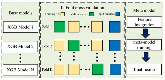
Figure 3.
Schematic diagram of the stacking ensemble model.
Using XGBoost as the meta-model , its optimization objective is given by
where is the regularization coefficient. The final wind speed prediction is given by
3.4. Validation
This study validates the retrieval performance of the proposed GAMSA-XGB-SE model through multi-level experiments. The experiments adopt a strict temporal separation validation strategy to ensure evaluation objectivity. The experimental design includes the following levels: first, the adaptive interval partitioning optimization process of the GAMSA algorithm is detailed; second, the performance of multiple machine learning algorithms is compared, including Support Vector Machine (SVM), Random Forest (RF), Multilayer Perceptron (MLP), Light Gradient Boosting Machine (LightGBM), XGBoost, and deep learning methods (CyGNSSnet [17] and FSNet [18]), to validate the overall superiority of the proposed method; third, the effects of different interval partitioning strategies are compared to verify the effectiveness of the GAMSA algorithm; finally, independent validation is performed using NDBC buoy observations.
All comparative methods employ the same data partitioning strategy and evaluation system, and performance is evaluated and compared using three metrics: mean absolute error (MAE), root mean square error (RMSE), and coefficient of determination (R2):
where represents the true sea surface wind speed value of the -th sample, is the corresponding predicted value by the model, and represent the mean values of all true values and predicted values, respectively, and n is the total number of samples.
4. Experimental Results
4.1. Partition Scheme
This section details the experimental implementation and results of the GAMSA algorithm. The GAMSA algorithm combines the global search capability of simulated annealing with the local optimization capability of gradient descent. After each acceptance of a new solution by simulated annealing, gradient descent is applied for local fine-grained search, ensuring both global exploration capability and rapid convergence to local optima. The specific algorithmic steps and parameters are summarized in Table 2.
Table 2.
Dynamic changes in key parameters during the GAMSA optimization process.
The parameter settings of the GAMSA algorithm during training are as described in Section 3.3, where the initial temperature is , the cooling rate is , the maximum number of iterations is , and the initial weights are , , , and .
4.2. Computational Efficiency Analysis
To evaluate the practical applicability of the proposed GAMSA-XGB-SE method, comprehensive computational benchmarking was conducted using the complete dataset (January–October 2024, approximately 33 M samples). All experiments were performed on identical hardware (Intel Xeon Gold 6248R CPU (3.0 GHz, 48 cores), 128 GB of RAM, and an NVIDIA GeForce RTX 5090 GPU with 32 GB of VRAM) to ensure fair comparison.
As shown in Table 3, GAMSA-XGB-SE demonstrates superior computational efficiency across multiple metrics. Despite incorporating adaptive interval partitioning and an ensemble architecture, its training time of 6.1 h is only 25.8% of that required by CyGNSSnet (23.6 h) and 21.4% of that required by FSNet (28.5 h). More critically for operational deployment, its inference performance is substantially faster: GAMSA-XGB-SE achieves 0.082 ms per sample on a CPU, compared with 1.114 ms on a GPU for CyGNSSnet and 1.203 ms on a GPU for FSNet. This means GAMSA-XGB-SE achieves a superior inference speed using only CPU resources, while deep learning methods require expensive GPU hardware, yet still perform slower: 13.6 times faster than CyGNSSnet and 14.7 times faster than FSNet. For batch processing of 10,000 samples, GAMSA-XGB-SE requires only 0.82 s on a CPU, whereas CyGNSSnet and FSNet require 11.14 s and 12.03 s on a GPU, respectively. This performance enables the processing of approximately 500,000 daily global observations from CYGNSS in approximately 41 s on a CPU alone, which is well within the requirements for near-real-time monitoring (typically defined as a processing delay under 3 h). With only 2.4 million parameters—substantially fewer than CyGNSSnet (7.7 million) and FSNet (9.2 million)—GAMSA-XGB-SE facilitates deployment on resource-constrained platforms. While it requires 4.2 GB of CPU memory (higher than the GPU memory footprint of deep learning methods: 966 MB of GPU for CyGNSSnet, and 1092 MB of GPU for FSNet), this reflects the architectural difference of maintaining multiple specialized sub-models simultaneously in memory for different wind speed intervals. Critically, GAMSA-XGB-SE operates entirely on a CPU without requiring specialized GPU hardware, significantly reducing deployment barriers for operational agencies. In contrast, deep learning methods necessitate specialized GPU hardware for both training and efficient inference, with combined memory footprints reaching 966 MB of GPU and 1756 MB of CPU for CyGNSSnet, and 1092 MB of GPU and 1850 MB of CPU for FSNet during the complete training pipeline.
Table 3.
Computational cost comparison of different methods.
5. Discussion
5.1. Physical Interpretation of GAMSA Interval Boundaries
To determine whether the wind speed interval boundaries identified by the GAMSA algorithm reflect actual shifts in sea surface scattering physics rather than merely statistical trends, we performed a differential analysis of the relationships between two key observables—normalized bistatic radar cross-section (NBRCS) and leading-edge slope (LES)—and wind speed. NBRCS is known to correlate strongly with sea surface roughness, while LES characterizes the waveform steepness, which is sensitive to ocean wave state and wind-driven conditions [12,33].
By computing the first-order derivatives (gradients) and second-order derivatives (curvature) of these observables with respect to wind speed, we identify the points where their response characteristics change significantly. As shown in Figure 4, NBRCS exhibits curvature extrema around 7.25 m/s and 18.25 m/s, while LES shows curvature extrema near 6.75 m/s and 18.25 m/s. These values align closely with the boundaries detected by the GAMSA algorithm at 7.06 m/s and 16.37 m/s, with deviations of less than 2 m/s in both cases. This strong agreement demonstrates that the algorithm effectively identifies the nonlinear transition points in the response functions of these observables, which correspond to shifts in the underlying sea surface scattering mechanisms.
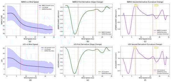
Figure 4.
Nonlinear characteristics of observables versus wind speed. Figure (a,d) show the smooth curves and ±1σ ranges for NBRCS and LES. Figure (b,e) display the first derivatives (gradient changes), and Figure (c,f) present the second derivatives (curvature changes). Red dashed lines indicate GAMSA boundaries, and orange boxes mark curvature extrema.
These experimental results provide a clear physical interpretation. The lower boundary (approximately 7 m/s) marks the transition from a smooth sea surface dominated by specular reflection to developing sea waves with mixed scattering mechanisms. The upper boundary (approximately 16 m/s) signifies the onset of fully developed turbulent conditions where diffuse scattering dominates, and geometric optical effects diminish. This evolutionary process is consistent with classical oceanographic theories regarding wind–wave development stages [12,32,33]. Importantly, these boundaries are derived entirely from data through optimization of interval coherence and separation, not preset by researchers, yet they align with genuine physical transitions in sea surface scattering behavior. This finding validates the scientific foundation of the GAMSA algorithm and demonstrates that adaptive interval partitioning captures meaningful environmental processes rather than statistical artifacts.
5.2. Comparison with Other Machine Learning Methods
To intuitively demonstrate the wind speed prediction capabilities of different machine learning methods, Figure 5 presents scatter plot comparisons between predicted and actual wind speeds for each method on the independent test set. Based on scatter dispersion, the SVM method (Figure 5a) exhibits an obvious fan-shaped divergent distribution with numerous points deviating from the diagonal line, with an RMSE of 2.33 m/s, MAE of 1.78 m/s, and R2 of only 0.3568, indicating the lowest prediction accuracy. The scatter convergence of the RF method (Figure 5b) and MLP method (Figure 5c) shows improvement, but numerous yellow and green scatter points still deviate from the diagonal line in the periphery of high-density regions, with RMSEs of 1.83 m/s and 1.91 m/s, MAEs of 1.37 m/s and 1.41 m/s, and R2 values of 0.6284 and 0.57, respectively. The scatter distributions of the LightGBM method (Figure 5d) and XGBoost method (Figure 5e) further converge toward the diagonal line, with RMSEs of 1.79 m/s and 1.77 m/s, MAEs of 1.32 m/s and 1.31 m/s, and R2 values of 0.6291 and 0.6293, although relatively obvious scattered points still exist in wind speed boundary regions (below 5 m/s and above 20 m/s). As deep learning methods, CyGNSSnet (Figure 5f) and FSNet (Figure 5g) show high-density scatter regions more compactly distributed along the diagonal line, with RMSEs of 1.63 m/s and 1.55 m/s, MAEs of 1.23 m/s and 1.17 m/s, and R2 values reaching 0.6827 and 0.7031, respectively, demonstrating significantly improved prediction consistency. Finally, the GAMSA-XGB-SE method (Figure 5h) achieves the best performance with the tightest scatter distribution along the diagonal line, with an RMSE of 1.43 m/s, an MAE of 1.05 m/s, and an R2 of 0.7770, representing the highest prediction accuracy among all methods.
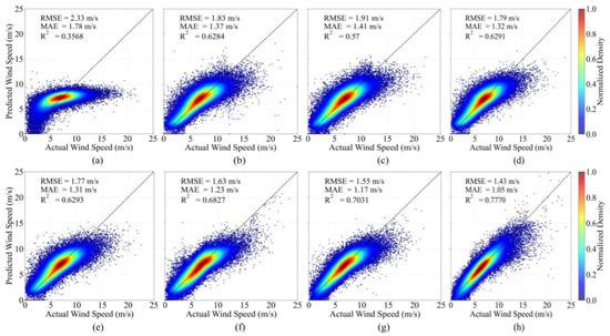
Figure 5.
Comparison of global wind speed retrieval scatter density plots for different methods on the independent test set. (a) SVM, (b) RF, (c) MLP, (d) LightGBM, (e) XGBoost, (f) CyGNSSnet, (g) FSNet, and (h) GAMSA-XGB-SE.
The proposed GAMSA-XGB-SE method (Figure 5h) exhibits the most outstanding performance, with high-density scatter regions highly concentrated along the diagonal line and the deviation distance of scattered points significantly smaller than other methods, achieving an RMSE of only 1.43 m/s, MAE of 1.05 m/s, and R2 of 0.7770. Compared with the global single XGBoost model, the proposed method reduces the RMSE by 19.2% and the MAE by 19.8% and improves the R2 by 23.5%. Compared with FSNet, the proposed method reduces the RMSE by 7.7% and the MAE by 10.3% and improves the R2 by 10.5%. This is attributed to the GAMSA algorithm’s effective capture of nonlinear characteristics across different wind speed ranges through adaptive interval modeling, combined with the stacking ensemble learning architecture that further suppresses the prediction bias of individual models. Particularly in the medium-to-high wind speed range of 10–20 m/s, the scatter distribution of the proposed method is the most compact, fully validating the generalization capability and robustness of the method.
To systematically quantify the performance of different methods across various wind speed intervals, Table 4 presents detailed RMSE statistics for traditional machine learning methods (SVM, RF, and MLP), ensemble learning methods (LightGBM and XGBoost), deep learning methods (CyGNSSnet and FSNet), and the proposed GAMSA-XGB-SE method on the independent test set (January–February 2025). The wind speed range is divided into seven intervals: 0–4 m/s, 4–8 m/s, 8–12 m/s, 12–16 m/s, 16–20 m/s, 20–24 m/s, and >24 m/s, enabling comprehensive evaluation of retrieval accuracy under different wind speed conditions.
Table 4.
RMSE comparison of different methods across wind speed intervals.
The statistical results in Table 4 demonstrate that the proposed GAMSA-XGB-SE method exhibits significant advantages across all wind speed intervals. For all samples, the proposed method achieves an RMSE of 1.43 m/s, representing reductions of 38.6%, 21.9%, 25.1%, 20.1%, and 19.2% compared with the machine learning methods (SVM, RF, MLP, LightGBM, and XGBoost, respectively), and reductions of 12.3% and 7.7% compared with the deep learning methods (CyGNSSnet and FSNet, respectively). Notably, among all comparative methods, XGBoost achieves the best performance among traditional machine learning methods, with an RMSE of 1.77 m/s, outperforming SVM, RF, MLP, and LightGBM, validating the rationale for selecting XGBoost as the base model for further optimization and ensemble in this study.
As wind speed increases, the performance gap between methods gradually expands. In the low-wind-speed interval (0–4 m/s), RMSE differences among methods are relatively small. The proposed method achieves an RMSE of 1.76 m/s, reaching the optimal level among all methods with reductions of 10.7–28.7% compared with machine learning methods and 9.3% and 6.9% compared with CyGNSSnet and FSNet, respectively.
In the medium-wind-speed intervals (4–12 m/s), the proposed method maintains stable low error levels, and its performance advantage begins to emerge. For the 4–8 m/s interval, the proposed method achieves an RMSE of 1.31 m/s, representing reductions of 8.4–13.8% compared with machine learning methods and 7.1% and 5.1% compared with CyGNSSnet and FSNet, respectively. For the 8–12 m/s interval, the RMSE is 1.48 m/s, representing reductions of 15.4–30.5% compared with machine learning methods and 14.0% and 9.8% compared with CyGNSSnet and FSNet, respectively.
In the transition interval (12–16 m/s), performance differentiation becomes more pronounced. The proposed method achieves an RMSE of 2.72 m/s, representing reductions of 25.1–44.0% compared with machine learning methods and 21.2% and 14.5% compared with CyGNSSnet and FSNet, respectively.
When wind speed exceeds 16 m/s, performance differences become increasingly significant. In the 16–20 m/s interval, the proposed method achieves an RMSE of 4.97 m/s, representing reductions of 16.3–33.0% compared with machine learning methods and 16.9% and 8.3% compared with CyGNSSnet and FSNet, respectively. In the 20–24 m/s interval, the RMSE is 7.42 m/s, representing reductions of 27.6–34.7% compared with machine learning methods and 20.6% and 15.9% compared with CyGNSSnet and FSNet, respectively. In the extremely high wind speed interval (>24 m/s), the RMSE is 12.05 m/s, demonstrating significant advantages over all comparative methods, with reductions of 27.4–39.7% compared with machine learning methods and 12.4% and 8.9% compared with CyGNSSnet and FSNet, respectively.
To comprehensively evaluate the retrieval accuracy and error distribution characteristics of different methods, Figure 6 and Figure 7 present the global sea surface wind speed spatial distributions and their prediction bias distributions relative to ERA5 reanalysis data, respectively, for eight retrieval methods on the independent test set (January–February 2025). As shown in Figure 6a, ERA5 data exhibit clear global wind speed distribution patterns, with distinct wind speed characteristics in mid-to-high latitude westerly wind belts and tropical convergence zones, as well as good spatial continuity, providing a reliable reference benchmark for method comparison.
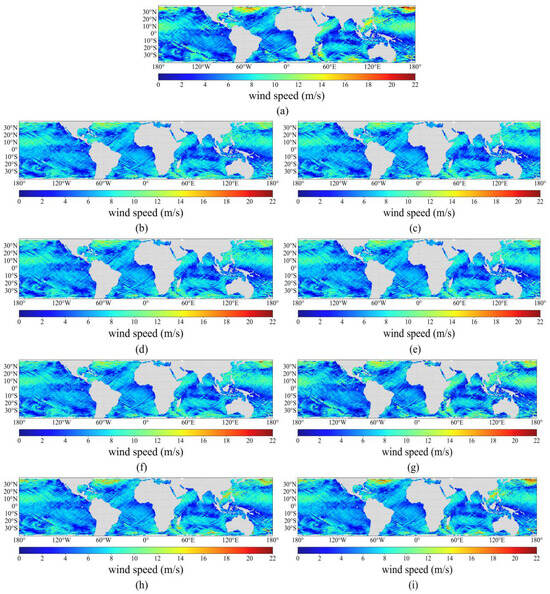
Figure 6.
Comparison of global wind speed distribution maps for different methods on the independent test set. (a) ERA5, (b) SVM, (c) RF, (d) MLP, (e) LightGBM, (f) XGBoost, (g) CyGNSSnet, (h) FSNet, and (i) GAMSA-XGB-SE.
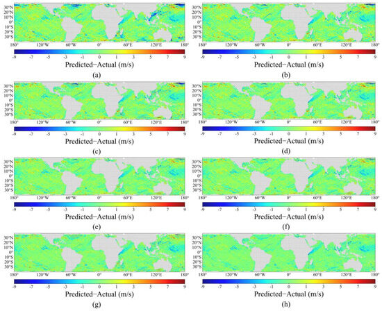
Figure 7.
Comparison of spatial distribution of prediction bias relative to ERA5 wind speed for different methods on the independent test set. (a) SVM, (b) RF, (c) MLP, (d) LightGBM, (e) XGBoost, (f) CyGNSSnet, (g) FSNet, and (h) GAMSA-XGB-SE.
Comparing the performance of different retrieval methods reveals obvious differences. Although the traditional machine learning method SVM (Figure 6b) captures the basic wind speed distribution pattern, it exhibits significant roughness in spatial details with insufficiently smooth wind speed gradient transitions. The bias distribution map (Figure 7a) shows that the SVM method produces substantial systematic biases over large ocean areas, particularly obvious underestimation in medium-to-high wind speed regions (blue areas), while some low-wind-speed regions show overestimation tendencies (red areas), resulting in spatially uneven bias distribution. The spatial distributions of the RF (Figure 6c) and MLP (Figure 6d) methods show relative improvement; however, their bias maps (Figure 7b,c) still reveal noticeable regional error accumulation, with large prediction biases in high-latitude regions and localized high wind speed areas, indicating that the spatial continuity of the wind speed field requires improvement.
The ensemble learning methods LightGBM (Figure 6e) and XGBoost (Figure 6f) demonstrate better spatial consistency and capture the macroscopic distribution characteristics of global wind speeds more effectively. The bias distributions (Figure 7d,e) show that systematic biases are somewhat reduced for these two methods, with a relatively uniform spatial distribution. However, deficiencies remain in local detail characterization and performance in extreme-value regions, as some ocean areas still exhibit patches of wind speed underestimation or overestimation, indicating that the model’s adaptability to different wind speed conditions requires further improvement.
The deep learning methods CyGNSSnet (Figure 6g) and FSNet (Figure 6h) achieve significant progress compared with traditional methods, with notably improved spatial continuity of the wind speed field and more accurate reproduction of wind speed gradient changes in mid-to-high latitude westerly wind belts. The bias distributions (Figure 7f,g) show that overall bias levels are further reduced for these two methods, with biases in most ocean areas controlled within a small range, presenting relatively uniform light green tones. However, in localized high-wind-speed core regions, these methods still exhibit certain degrees of smoothing effects and systematic underestimation, with sporadic blue patches still visible in the bias maps, indicating limited capability in characterizing extreme wind speed events.
In contrast, the proposed GAMSA-XGB-SE method (Figure 6i) demonstrates optimal global wind speed retrieval capability, with its spatial distribution pattern highly consistent with ERA5 reference data. The wind speed field exhibits excellent spatial smoothness and continuity, effectively avoiding the discontinuous jumps common in traditional methods and achieving natural, smooth transitions globally. More importantly, the bias distribution map (Figure 7h) clearly shows that the proposed method achieves optimal bias control globally, presenting large areas of uniform light green tone, indicating high agreement between predicted and true values. In key climate regions, such as mid-to-high latitude westerly wind belts and tropical easterly wind belts, the proposed method accurately captures spatial gradient changes and local detail characteristics of wind speed, with extremely uniform bias distribution and virtually no significant systematic overestimation or underestimation. Particularly in high-wind-speed core regions such as the Southern Hemisphere westerly wind belt, the method accurately reproduces wind speed peaks without obvious blue underestimation areas in the bias map, avoiding both the excessive smoothing of traditional methods and the local overfitting that may occur with deep learning methods. Meanwhile, in low-wind-speed regions such as equatorial doldrums, the proposed method maintains high retrieval accuracy and stable bias control, with uniform and reasonable wind speed field distribution and no obvious regional systematic bias.
5.3. Performance Comparison Analysis of Different Partitioning Strategies
To further validate the effectiveness of the GAMSA-XGB-SE method, comprehensive comparative analyses were conducted on the independent test set against the global single XGBoost model, the 10 m/s threshold partitioning method mentioned in the Introduction, the 15 m/s threshold partitioning method, and the equal-sample three-interval partitioning method.
Figure 8 shows the RMSE variation trends across wind speed intervals for the proposed GAMSA-XGB-SE method and other schemes. As shown in the figure, the RMSE for all methods exhibits an increasing trend with wind speed, but with significant differences in the magnitude of increase. The proposed GAMSA-XGB-SE method maintains the lowest RMSE level across all wind speed intervals, particularly demonstrating obvious advantages in key intervals such as 8–12 m/s, 12–16 m/s, and 16–20 m/s. The figure also annotates sample quantities in each interval, revealing that in medium-wind-speed intervals (8–16 m/s) with sufficient sample sizes, the performance advantage of the proposed method is more stable. When the wind speed exceeds 20 m/s, although the RMSE for all methods increases significantly, the proposed method still maintains optimal performance, fully demonstrating the effectiveness of the adaptive partitioning strategy compared with other partitioning strategies.

Figure 8.
Variation trends of RMSE performance for different methods across wind speed intervals on the independent test set.
Figure 9 presents a more intuitive comparison of RMSE performance across wind speed intervals for different partitioning schemes in bar chart form. The figure clearly shows that the RMSE for the proposed GAMSA-XGB-SE method is significantly lower than other fixed partitioning schemes across all wind speed intervals. In the low-wind-speed interval (0–8 m/s), differences among methods are relatively small, with the RMSEs all controlled within 2 m/s. In the medium-wind-speed interval (8–16 m/s), the performance gap between methods begins to emerge, and the advantage of the proposed method gradually becomes apparent. In the high-wind-speed region (>16 m/s), the RMSE gap between different methods expands dramatically, while the proposed method maintains the RMSE at a relatively low level with highly significant performance advantages. This comparative result indicates that the interval partitioning strategy based on adaptive multi-objective optimization can effectively adapt to data characteristics under different wind speed conditions, achieving more balanced and superior retrieval performance across the entire wind speed range.
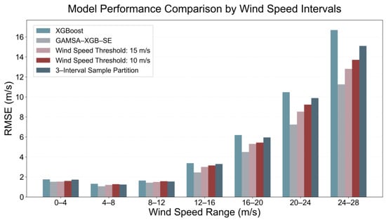
Figure 9.
Direct comparison of RMSE performance for different methods across wind speed intervals on the independent test set.
5.4. Independent Validation with Buoy Observation Data
This study selected 15 buoy stations located within the CYGNSS coverage area, covering different ocean regions including the Atlantic Ocean, Pacific Ocean, and Gulf of Mexico, with a time range of January–February 2025. After matching with CYGNSS and ERA5 data, approximately 9421 valid matched samples were obtained.
Figure 10 presents scatter plots comparing wind speeds estimated by different methods with NDBC buoy measurements. As shown in the figure, ERA5 reanalysis data (Figure 10a), as the reference dataset, exhibit good consistency, with an RMSE of 1.30 m/s. The single XGBoost model (Figure 10b) shows greater scatter dispersion, with an RMSE of 1.77 m/s, representing the highest prediction error. The deep learning method CyGNSSnet (Figure 10c) shows an improved scatter distribution with an RMSE of 1.69 m/s. FSNet (Figure 10d) further enhances prediction accuracy, with the RMSE reduced to 1.65 m/s and notably improved scatter concentration. The scatter distribution of the proposed GAMSA-XGB-SE method (Figure 10e) is more compact and concentrated near the diagonal line, with an RMSE of 1.52 m/s, MAE of 1.11 m/s, and R2 of 0.79, representing error reductions of 14.1% compared with the single XGBoost model, 10.1% compared with CyGNSSnet, and 7.9% compared with FSNet, demonstrating good consistency with buoy observations. These results indicate that the proposed method not only performs excellently when compared with reanalysis data but also exhibits stable and reliable prediction performance when validated against completely independent in situ observations, proving the effectiveness of the adaptive interval partitioning and ensemble learning strategy for practical applications.
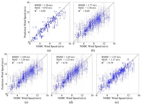
Figure 10.
Comparison of wind speeds estimated by different methods with NDBC buoy measurements. (a) ERA5, (b) single XGBoost, (c) CyGNSSnet, (d) FSNet, and (e) GAMSA-XGB-SE.
6. Conclusions
This study addresses the problems in GNSS-R sea surface wind speed retrieval, where unified modeling across the entire wind speed range cannot effectively capture the physical property differences across different wind speed intervals, while current interval partitioning relies on empirical thresholds detached from the actual data distribution and faces difficulties in determining the interval assignment for new samples during prediction. A GAMSA-XGB-SE wind speed retrieval method is proposed. Through systematic theoretical analysis, algorithm design, and experimental validation, the following main research achievements have been obtained:
- Targeting the limitation of traditional empirical threshold partitioning methods being isolated from data distribution characteristics, this study proposes the GAMSA adaptive interval partitioning algorithm. This algorithm integrates gradient-guided local search into the global exploration process of simulated annealing, constructs a multi-objective optimization function that comprehensively considers prediction error distribution, number of intervals, sample distribution uniformity, and minimum sample requirements, and achieves data-driven optimal wind speed interval partitioning through a fixed normalization strategy and dynamic weight adjustment mechanism.
- Targeting the difficulty of matching new samples with sub-models in traditional interval partitioning methods, this study constructs a stacking ensemble learning architecture to integrate the prediction results of multiple wind speed interval sub-models. Through K-fold cross-validation to generate meta-features and train a second-level meta-model, smooth fusion of interval models is achieved, solving the automatic sample matching problem in practical applications and significantly improving the engineering practicability and prediction stability of the method.
- Based on CYGNSS L1 data and ERA5 reanalysis data, validation was conducted using a strict temporal separation strategy (January–October 2024 for training, November–December 2024 for validation, and January–February 2025 for independent testing). The results demonstrate that compared with the traditional global single XGBoost model, the proposed method reduces the RMSE from 1.77 m/s to 1.43 m/s (a 19.2% improvement) and improves the R2 from 0.6293 to 0.7770 (a 23.5% enhancement); compared with CyGNSSnet and FSNet, the RMSE is reduced by 12.3% and 7.7%, respectively, exhibiting superior stability in high-wind-speed regimes (>16 m/s). In terms of computational efficiency, GAMSA-XGB-SE requires only 6.1 h for training (representing 25.8% and 21.4% of the CyGNSSnet and FSNet training times, respectively) and achieves a CPU inference speed of 0.082 ms per sample, which is 13.6 times faster than CyGNSSnet and 14.7 times faster than FSNet running on a GPU, enabling the processing of a full day’s global CYGNSS observations (approximately 500,000 samples) in approximately 41 s on standard CPU hardware, thereby satisfying near-real-time operational requirements. The GAMSA adaptive partitioning method significantly outperforms fixed partitioning schemes across all wind speed intervals, with particularly pronounced advantages in high-wind-speed regions (>20 m/s). Independent validation against NDBC buoy measurements yields an RMSE of 1.52 m/s and an R2 of 0.79. Global spatial distribution analysis indicates that the proposed method exhibits excellent robustness across diverse oceanic regions.
In summary, through the organic combination of adaptive interval modeling and ensemble learning strategies, this study not only solves the problem of single models struggling to adapt to different wind speed interval characteristics but also overcomes the empirical dependence and engineering application challenges of traditional interval partitioning methods, achieving higher retrieval accuracy and better stability across the entire wind speed range, providing new methodological support for high-precision monitoring of global ocean wind fields.
Although the proposed method represents a significant advance, its performance under extreme wind conditions (>30 m/s), characteristic of tropical cyclone inner cores, has not been adequately benchmarked due to data scarcity. Future work must prioritize a more rigorous evaluation in these critical regimes by incorporating extreme wind samples from complementary sources. A key step is to extend the application of this method, currently demonstrated on CYGNSS data, to other GNSS-R satellite platforms [46,47] to assess its generalizability. Concurrently, cross-validation against independent datasets—such as hurricane hunter aircraft measurements, high-resolution SAR wind retrievals, and operational hurricane model analyses—is essential to establish robustness under severe storms. This comprehensive validation is a critical prerequisite for the operational adoption and broader application of GNSS-R technology in tropical cyclone forecasting, ocean monitoring, and meteorological services [48,49].
Author Contributions
Conceptualization, Y.J. and Y.Z.; methodology, Y.Z.; software, Y.Z.; validation, Y.J., Y.Z. and X.S.; formal analysis, Y.J.; investigation, Y.Z.; resources, S.Z.; data curation, X.S.; writing—original draft preparation, Y.Z.; writing—review and editing, Y.Z.; visualization, Y.Z.; supervision, S.Z.; project administration, X.S.; funding acquisition, Y.J. All authors have read and agreed to the published version of the manuscript.
Funding
This research was supported by the Guangxi Science and Technology Program (grant nos. AB23026120, ZY23055048, AA24263006, AA24206043, and AA24263010), the Guangxi Science and Technology Base and Talent Special Project (grant no. AD25069103), the National Natural Science Foundation of China (grant nos. U23A20280, 62471153, and U25A20397), the Nanning Scientific Research and Technology Development Program (grants nos. 20231029 and 20231011), the Industry-University-Research Project (grant nos. CYY-HT2023-JSJJ-0023-1 and CYY-HT2023-JSJJ-0024-1), the Guangxi Zhuang Autonomous Region Major Talent Project, and the Beidou Location Service and Border-Coastal Defense Safety Application Engineering Research Center of Guangxi Universities.
Data Availability Statement
The data presented in this study are openly available in https://search.earthdata.nasa.gov/search (accessed on 1 November 2025), https://cds.climate.copernicus.eu/datasets/reanalysis-era5-pressure-levels?tab=download (accessed on 1 November 2025), and https://www.ndbc.noaa.gov/ (accessed on 1 November 2025).
Conflicts of Interest
Author Xiyan Sun was employed by the company Nanning GUET Electronics Technology Research Institute Co., Ltd. The remaining authors declare that the research was conducted in the absence of any commercial or financial relationships that could be construed as a potential conflict of interest.
References
- Zhou, L.; Zheng, G.; Yang, J.; Li, X.; Zhang, B.; Wang, H.; Chen, P.; Wang, Y. Sea surface wind speed retrieval from textures in synthetic aperture radar imagery. IEEE Trans. Geosci. Remote Sens. 2022, 60, 4200911. [Google Scholar] [CrossRef]
- Zheng, C.W.; Li, C.Y.; Pan, J.; Liu, M.Y.; Xia, L.L. An overview of global ocean wind energy resource evaluations. Renew. Sustain. Energy Rev. 2016, 53, 1240–1251. [Google Scholar] [CrossRef]
- Dai, S.; Wang, C.; Luo, F. Identification and learning control of ocean surface ship using neural networks. IEEE Trans. Ind. Inform. 2012, 8, 801–810. [Google Scholar] [CrossRef]
- Barnier, B.; Domina, A.; Gulev, S.; Molines, J.-M.; Maitre, T.; Penduff, T.; Le Sommer, J.; Brasseur, P.; Brodeau, L.; Colombo, P. Modelling the impact of flow-driven turbine power plants on great wind-driven ocean currents and the assessment of their energy potential. Nat. Energy 2020, 5, 240–249. [Google Scholar] [CrossRef]
- Zhang, L.; Shi, H.; Wang, Z.; Yu, H.; Yin, X.; Liao, Q. Comparison of wind speeds from spaceborne microwave radiometers with in situ observations and ECMWF data over the global ocean. Remote Sens. 2018, 10, 425. [Google Scholar] [CrossRef]
- Nezhad, M.; Neshat, M.; Heydari, A.; Razmjoo, A.; Piras, G.; Garcia, D.A. A new methodology for offshore wind speed assessment integrating Sentinel-1, ERA-interim and in-situ measurement. Renew. Energy 2021, 172, 1301–1313. [Google Scholar] [CrossRef]
- Tang, W.; Liu, W.T.; Stiles, B.W. Evaluation of high-resolution ocean surface vector winds measured by QuikSCAT scatterometer in coastal regions. IEEE Trans. Geosci. Remote Sens. 2004, 42, 1762–1769. [Google Scholar] [CrossRef]
- Meissner, T.; Wentz, F.J. Wind-vector retrievals under rain with passive satellite microwave radiometers. IEEE Trans. Geosci. Remote Sens. 2009, 47, 3065–3083. [Google Scholar] [CrossRef]
- Zhang, S.W.; Yang, W.C.; Xin, Y.Z.; Wang, R.X.; Li, C. Research progress of buoy-based ocean observation system. Chin. Sci. Bull. 2019, 64, 2963–2973. [Google Scholar]
- Wu, Y.H.; Liu, R.P.; Hua, B.; Wang, F. Design of global time-limited revisit constellation configuration. Comput. Simul. 2020, 37, 87–91+101. [Google Scholar]
- Martin-Neira, M. A passive reflectometry and interferometry system (PARIS): Application to Ocean Altimetry. ESA J. 1993, 17, 331–355. [Google Scholar]
- Zavorotny, V.U.; Voronovich, A.G. Scattering of GPS signals from the ocean with wind remote sensing application. IEEE Trans. Geosci. Remote Sens. 2000, 38, 951–964. [Google Scholar] [CrossRef]
- Foti, G.; Gommenginger, C.; Jales, P.; Unwin, M.; Shaw, A.; Robertson, C.; Rosello, J. Spaceborne GNSS reflectometry for ocean winds: First results from the UK TechDemoSat-1 mission. Geophys. Res. Lett. 2015, 42, 5435–5441. [Google Scholar] [CrossRef]
- Wang, X.; Sun, Q.; Zhang, X.J.; Lv, D.R.; Shao, L.J.; Hu, X.; Ruffini, G.; Dunne, S.; Francois, S. China’s first shore-based GNSS-R ocean remote sensing experiment. Chin. Sci. Bull. 2008, 53, 589–592. [Google Scholar]
- Liu, L.; Xia, J.; Bai, W.; Sun, Y.; Du, Q.; Luo, L. Influence of evaporation duct on the effective scattering area of GNSS sea surface reflected signals. Chin. J. Geophys. 2019, 62, 499–507. [Google Scholar]
- Yu, K. Theory and Practice of GNSS Reflectometry; Springer Nature: Berlin/Heidelberg, Germany, 2021; pp. 1–376. [Google Scholar]
- Clarizia, M.P.; Ruf, C.S.; Jales, P.; Gommenginger, C. Spaceborne GNSS-R Minimum Variance Wind Speed Estimator. IEEE Trans. Geosci. Remote Sens. 2014, 52, 6829–6843. [Google Scholar] [CrossRef]
- Bu, J.; Yu, K.; Zhu, Y.; Qian, N.; Chang, J. Developing and testing models for sea surface wind speed estimation with GNSS-R delay doppler maps and delay waveforms. Remote Sens. 2020, 12, 3760. [Google Scholar] [CrossRef]
- Gleason, S.; Johnson, J.; Ruf, C.; Bussy-Virat, C. Characterizing background signals and noise in spaceborne GNSS refection ocean observations. IEEE Geosci. Remote Sens. Lett. 2020, 17, 587–591. [Google Scholar] [CrossRef]
- Ma, L.; Liu, Y.; Zhang, X.; Ye, Y.; Yin, G.; Johnson, B.A. Deep learning in remote sensing applications: A meta-analysis and review. ISPRS J. Photogramm. Remote Sens. 2019, 152, 166–177. [Google Scholar] [CrossRef]
- Li, X.H.; Yang, D.K.; Yang, J.S.; Zheng, G.; Han, G.Q.; Nan, Y.; Li, W.Q. Analysis of coastal wind speed retrieval from CYGNSS mission using artificial neural network. Remote Sens. Environ. 2021, 260, 112454. [Google Scholar] [CrossRef]
- Reynolds, J.; Clarizia, M.P.; Santi, E. Wind speed estimation from CYGNSS using artifcial neuralnetworks. IEEE J. Sel. Top. Appl. Earth Obs. Remote Sens. 2020, 13, 708–716. [Google Scholar] [CrossRef]
- Asgarimehr, M.; Arnold, C.; Weigel, T.; Ruf, C.; Wickert, J. GNSS Reflectometry global ocean wind speed using deep learning: Development and assessment of CyGNSSnet. Remote Sens. Environ. 2022, 269, 112801. [Google Scholar] [CrossRef]
- Chen, K.; Zhou, Y.; Li, S.; Wang, P.; Li, X. Exploiting Frequency-Domain Information of GNSS Reflectometry for Sea Surface Wind Speed Retrieval. IEEE Trans. Geosci. Remote Sens. 2023, 61, 4205713. [Google Scholar] [CrossRef]
- Zhang, Y.; Yin, J.W.; Yang, S.H.; Meng, W.T.; Han, Y.L.; Yan, Z.Y. High wind speed inversion model of CYGNSS sea surface data based on machine learning. Remote Sens. 2021, 13, 3324. [Google Scholar] [CrossRef]
- Gleason, S.; Ruf, C.S.; O’Brien, A.; McKague, D.S. The CYGNSS level 1 calibration algorithm and error analysis based on on-orbit measurements. IEEE J. Sel. Top. Appl. Earth Obsserv. Remote Sens. 2019, 12, 37–49. [Google Scholar] [CrossRef]
- Xue, J.; Sun, R. GNSS-R based Partitioned Sea Surface Wind Speed Monitoring Model. J. Phys. Conf. Ser. 2025, 2999, 012043. [Google Scholar] [CrossRef]
- Wang, C.; Yu, K.; Qu, F.; Bu, J.; Han, S.; Zhang, K. Spaceborne GNSS-R Wind Speed Retrieval Using Machine Learning Methods. Remote Sens. 2022, 14, 3507. [Google Scholar] [CrossRef]
- Ruf, C.; Unwin, M.; Dickinson, J.; Rose, R.; Rose, D.; Vincent, M.; Lyons, A. CYGNSS: Enabling the future of hurricane prediction [Remote sensing Satellites]. IEEE Geosci. Remote Sens. Mag. 2013, 1, 52–67. [Google Scholar] [CrossRef]
- Ruf, C.S.; Chew, C.; Lang, T.; Morris, M.G.; Nave, K.; Ridley, A.; Balasubramaniam, R. A new paradigm in Earth environmental monitoring with the CYGNSS small satellite constellation. Sci. Rep. 2018, 8, 8782. [Google Scholar] [CrossRef] [PubMed]
- Ruf, C. CYGNSS Handbook; Michigan Publishing Services: Ann Arbor, MI, USA, 2022. [Google Scholar]
- Asharaf, S.; Waliser, D.E.; Posselt, D.J.; Ruf, C.S.; Zhang, C.; Putra, A.W. CYGNSS Ocean Surface Wind Validation in the Tropics. J. Atmos. Ocean. Technol. 2021, 38, 711–724. [Google Scholar] [CrossRef]
- Ruf, C.; Asharaf, S.; Balasubramaniam, R.; Gleason, S.; Lang, T.; McKague, D.; Twigg, D.; Waliser, D. In-orbit performance of the constellation of CYGNSS hurricane satellites. Bull. Am. Meteorol. Soc. 2019, 100, 2009–2023. [Google Scholar] [CrossRef]
- Liu, E.; Sun, R.; Wang, Y. Improved GNSS-R Wind Speed Retrieval Model Considering the Relationship Between Wind Direction and Reflection Point Trajectory. J. Phys. Conf. Ser. 2025, 2999, 012042. [Google Scholar] [CrossRef]
- Clarizia, M.P.; Ruf, C.S. Wind speed retrieval algorithm for the cyclone global navigation satellite system (CYGNSS) Mission. IEEE Trans. Geosci. Remote Sens. 2016, 54, 4419–4432. [Google Scholar] [CrossRef]
- Liu, Y.X.; Collett, I.; Morton, Y.J. Application of neural network to GNSS-R wind speed retrieval. IEEE Trans. Geosci. Remote Sens. 2019, 57, 9756–9766. [Google Scholar] [CrossRef]
- Clarizia, M.P.; Ruf, C.S. Statistical derivation of wind speeds from CYGNSS data. IEEE Trans. Geosci. Remote Sens. 2020, 58, 3955–3964. [Google Scholar] [CrossRef]
- Ruf, C.S.; Balasubramaniam, R. Development of the CYGNSS geophysical model function for wind speed. IEEE J. Sel. Top. Appl. Earth Observ. Remote Sens. 2019, 12, 66–77. [Google Scholar] [CrossRef]
- Hersbach, H.; Bell, B.; Berrisford, P.; Hirahara, S.; Horányi, A.; Muñoz-Sabater, J.; Nicolas, J.; Peubey, C.; Radu, R.; Schepers, D.; et al. The ERA5 global reanalysis. Quart. J. Roy. Meteorol. Soc. 2020, 146, 1999–2049. [Google Scholar] [CrossRef]
- Molteni, F.; Buizza, R.; Palmer, T.N.; Petroliagis, T. The ECMWF ensemble prediction system: Methodology and validation. Quart. J. Roy. Meteorol. Soc. 1996, 122, 73–119. [Google Scholar] [CrossRef]
- ERA5 Hourly Data on Single Levels From 1940 to Present, C.D.S. In Copernicus Climate Change Service; Copernicus Climate Change Service (C3S) Climate Data Store (CDS): Shinfield, UK, 2023.
- Aj-Fernández, S.; Ramos-Llordén, G.; Yushkevich, P.A. Image representation and 2D signal processing. In Medical Image Analysis; Frangi, A.F., Prince, J.L., Sonka, M., Eds.; Academic: New York, NY, USA, 2024; pp. 115–143. [Google Scholar]
- Ricciardulli, L.; Manaster, A.; Lindsley, R. Investigation of a calibration change in the ocean surface wind measurements from the TAO buoy array. Bull. Amer. Meteorol. Soc. 2025, 106, E242–E260. [Google Scholar] [CrossRef]
- Aarts, E.; Korst, J. Simulated annealing and Boltzmann machines. In Handbook of Brain Theory & Neural Networks; MIT Press: Cambridge, MA, USA, 1989; pp. 106–109. [Google Scholar]
- Husin, S.F.; Mamat, M.; Ibrahim, M.A.H.; Rivaie, M. A modification of steepest descent method for solving large-scaled unconstrained optimization problems. Int. J. Eng. Technol. 2018, 7, 72. [Google Scholar] [CrossRef]
- Tu, J.; He, X.; Xu, X.; Song, M.; Xu, X. Assessment of Tianmu-1 multi-GNSS-R global soil moisture products. Adv. Space Res. 2025, 76, 1476–1491. [Google Scholar] [CrossRef]
- Jing, C.; Li, W.; Wan, W.; Lu, F.; Niu, X.; Chen, X.; Rius, A.; Cardellach, E.; Ribó, S.; Liu, B.; et al. A review of the BuFeng-1 GNSS-R mission: Calibration and validation results of sea surface and land surface. Geo-Spat. Inf. Sci. 2024, 27, 638–652. [Google Scholar] [CrossRef]
- Peng, J.; Li, W.; Cardellach, E.; Marigold, G.; Clarizia, M.-P. Signal coherence and water detection algorithms for the ESA HydroGNSS mission. IEEE Trans. Geosci. Remote Sens. 2024, 62, 5801218. [Google Scholar] [CrossRef]
- Jia, T.; Xu, J.; Weng, F.; Huang, F. Retrieval of sea surface wind speed from CYGNSS data in tropical cyclone conditions using physics-guided artificial neural network and storm-centric coordinate information. IEEE J. Sel. Top. Appl. Earth Observ. Remote Sens. 2025, 18, 6746–6759. [Google Scholar] [CrossRef]
Disclaimer/Publisher’s Note: The statements, opinions and data contained in all publications are solely those of the individual author(s) and contributor(s) and not of MDPI and/or the editor(s). MDPI and/or the editor(s) disclaim responsibility for any injury to people or property resulting from any ideas, methods, instructions or products referred to in the content. |
© 2025 by the authors. Licensee MDPI, Basel, Switzerland. This article is an open access article distributed under the terms and conditions of the Creative Commons Attribution (CC BY) license (https://creativecommons.org/licenses/by/4.0/).