Wind, Water Level, and Fluid Mud Thresholds in Lake Apopka, Florida

Abstract

A study was undertaken at Lake Apopka in Florida to assess the minimum water depth required to contain a wind-induced episodic rise of fluid mud. In a year-long investigation, measurements were made at the mean water depth of 1.3 m to record the variation of suspended sediment concentration due to bed erosion and settling of the flocculated matter. The height of rise is defined as the elevation above the bed at which the mud floc volume fraction is at the threshold between the so-called flocculation settling and hindered settling regimes. The rise, which is considered significant when fluid mud occupies the 0.2 m high benthic boundary layer (BBL), occurs when the threshold wind exceeds about 9 m s⁻¹ corresponding to a 4% cumulative probability of occurrence. Predictive modeling suggests that in 2 m water depth the required wind would be about 14 m s⁻¹ with a low probability of 2%. Moreover, a transition occurs from wave-dominant resuspension at low depths to current-dominance in deeper water, which likely influences BBL dynamics with potential effects on the benthic biota. Provided a higher than present depth can be sustained in the large lake, the deduced relationship between fluid mud rise, wind speed, and water depth makes it feasible to select the depth at which the frequency of fluid mud occupying the BBL remains acceptably low. The developed protocol is general enough to be applicable to other similar shallow lakes where fluid mud rise must be contained.

1. Introduction

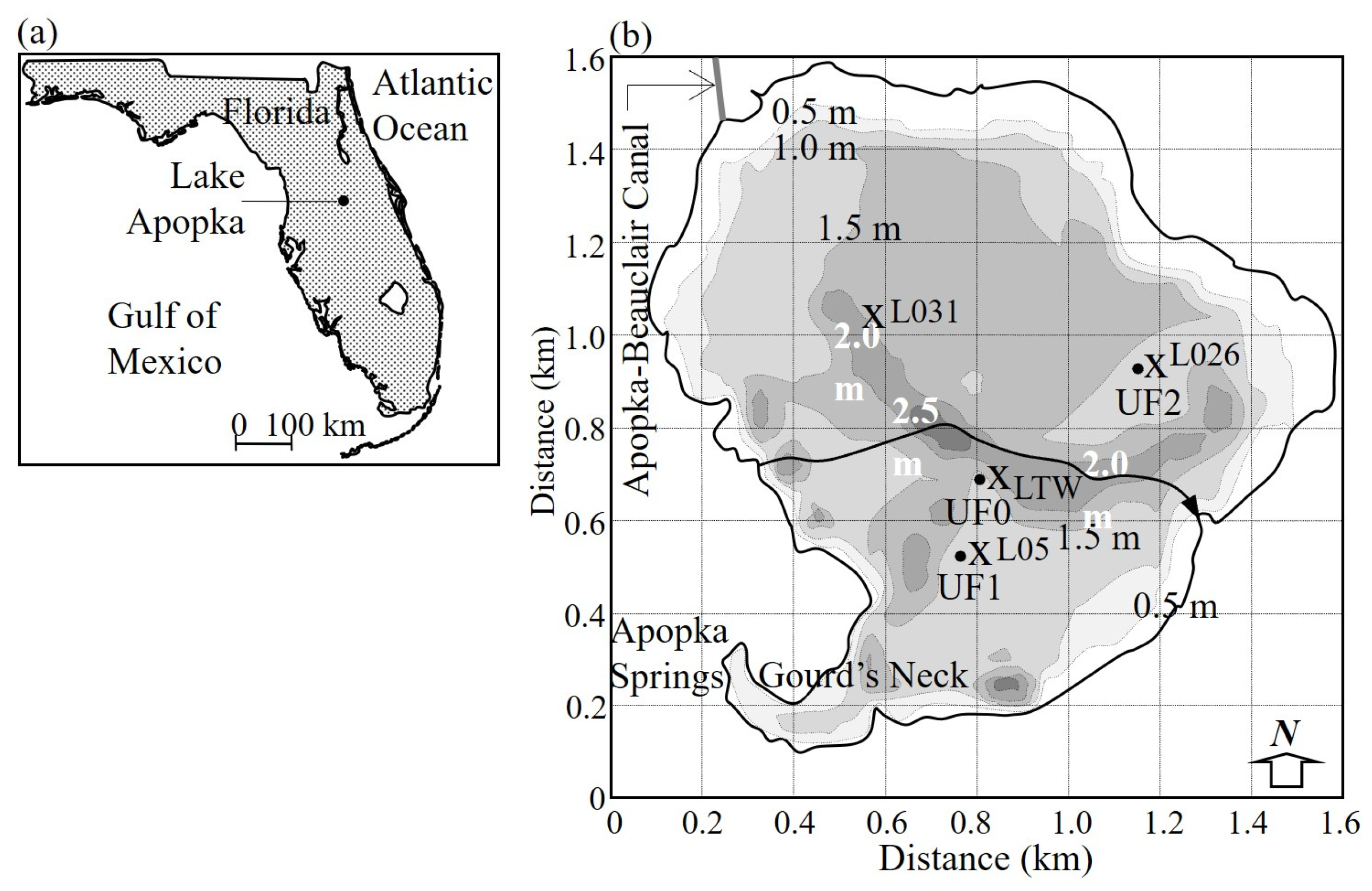
In shallow lakes with organic-rich cohesive sediment, resuspension of flocs is due to wind-induced waves and currents. Thus, nutrients and contaminants, if sequestered in the bottom sediment, may contribute to algal blooms, growth of macrophytes, and high toxicity [1,2,3]. In Lake Apopka, about ~25 km northwest of the Orlando metropolitan area in Florida (28°37′8.39″ N, −81°37′11.39″ W; Figure 1a,b), the emergence of phosphate associated with resuspended flocs has been a persistent concern due to high concentrations of total phosphorus in the bottom sediment. Phosphate accumulation is believed to have resulted mainly due to discharges from a large farming area on a floodplain marsh north of the lake [4]. As a result, the bottom mud over an originally sandy substrate has increased in thickness to as much as 2 m.

From the viewpoint of sediment movement in the lake, of particular interest is the occurrence of fluid mud confirmed in a study of the bottom sediment [5]. In that regard, as it contributes most of the suspended sediment mass, decreasing the effect of wind by increasing the water depth is one way by which mud in this form can be contained. However, as no study of sediment dynamics had been made in the lake, questions concerning the required minimum water depth were unaddressed. The aim of the present investigation was to ascertain the dependence of fluid mud height and frequency on wind speed and water depth. The study relied on a field measurement campaign, laboratory tests to characterize the sediment properties, and the use of a numerical hydrodynamic/sediment transport model for predictive purposes.

This presentation includes the following: (1) methods used for the field investigation and hydrodynamic modeling; (2) the lake’s physical setting including wind, waves, and currents; (3) sediment properties; (4) simulations of lake hydrodynamics and fluid mud rise as functions of wind speed and mean water depth; and (5) observations on the required water depth to contain fluid mud rise. The full study is reported in [6]. For the present work, the analyses of both field and laboratory measurements including modeling were partially re-evaluated. Moreover, the work focusses on lake-specific relationships between the wind speed, water depth, and the probability of occurrence of fluid mud. The investigation generally follows a framework for such studies in estuaries, bays, and lakes proposed by [7].

2. Measurement and Simulation Methods

2.1. Measurements

The lake, with a surface area of ~125 km², is fed by three freshwater sources along its western shoreline, the main being Apopka Springs (Figure 1b), which, however, has a marginal influence on the wind-driven lake hydrodynamics. The Apopka–Beauclair Canal with a flow control structure is the only outlet. The field campaign included time-series measurements of flow and suspended sediment and sediment property measurements both in situ and in the laboratory. During the period selected for analysis of the time series, the lake’s mean water depth was 1.3 m, although it is known to vary between 0.5 m and 2.5 m [5]. These characteristic depths depend on the physiography of the lake, freshwater sources, and the wind field. Bottom characterization was accomplished by push coring near stations UF0, UF1, and UF2 (Figure 1b), which consisted of submerged steel tripods anchored to the bottom. At these three locations, water level, currents, and suspended sediment concentration (SSC) were measured. Three of the four core locations (L05, L26, and L31) were reoccupations of the sites [5], and an additional site (LTW) was established 100 m east of UF0. Replicate cores were collected at all four sites on 30 August 2007 and 13 May 2008. Lab procedures for the radiometric, gravimetric, and rheometric analyses of the cores have been outlined in [6].

UF0, where the depth of water was 1.3 m, i.e., equal to the mean depth in the lake, was the primary station next to a meteorological tower maintained by the St. Johns River Water Management District, Palatka. At that site, an acoustic Doppler current profiler (ADCP), an SBE water level (wave) sensor, and an optical backscatter sensor (OBS) were mounted, and hourly 3-min average wind speed at 10 m elevation was obtained from the tower. The OBS elevation was set to be 0.2 m above the sediment bed based on, as described later, the estimated height of the benthic boundary layer (BBL) [8]. At both UF1 and UF2, an ADCP and an OBS were mounted. Altogether nine deployments, each lasting several weeks, were made between 25 July 2007 and 16 September 2008. Sampling was carried out every hour at frequencies listed in

Table 1. Transducers for water level, currents, and suspended sediment.

Parameter	Make	Model	Sampling Frequency (Hz)
Water level	Sea-Bird Electronics	SBE 26-03	4
Current velocity	RD Instruments	Workhorse Sentinel (ADCP)	0.5, 1
Suspended sediment	D & A Instruments	OBS-3	1
		OBS-5+	25

. As a measure against biofouling, the transducers were retrieved, cleaned, and reinstalled every two weeks. Although the recordings were meant to be continuous, equipment malfunction and weather led to several discontinuities, particularly at UF1 and UF2. At UF0, floc population diameters and settling velocities and densities were determined by using the LabSFLOC apparatus (HR Wallingford, Wallingford, UK) [9]. Rheometric data were obtained from a Brookfield LVDV-1 Prime viscometer (Brookfield Engineering Labs, Middleboro, MA, USA). An Aqua-Vu (Nature Vision, Inc., Brainerd, MN, USA) underwater video camera enabled the detection of the bed/water interface.

2.2. Simulations

Like most lakes with organic-rich muddy sediment in Florida, Apopka (mean organic content 62%) would be classified as “low-concentration”, with the SSC at a mid-depth normally lower than about 10⁻¹ kg m⁻³, while the present interest was in examining the rare fluid mud forming occasions when the SSC exceeded about 3 kg m⁻³. The same mode of episodic resuspension has been observed in other shallow lakes in Florida, including the largest, Lake Okeechobee, where, like Lake Apopka, the throughput of freshwater has an overall minor influence on wind-induced resuspension. In such lakes, localized variation of the SSC with wind has been simulated reasonably by 1D-vertical modeling of erosion and settling, while recognizing that the variability in the organic fraction of sediment has a significant effect on fluid mud properties and on the rates of sediment erosion and deposition [10]. It is the key reason why modeling, even though generic, must be calibrated with site-specific measurements. As a hydroinformatic tool for examining lake-wide resuspension, the 3D Environmental Fluid Dynamics Code (EFDC, Version 1.01) together with a coupled routine for sediment transport was used to simulate the waves, hydrostatic currents, and the SSC. The full modeling methodology is given in [11]. A wave routine was appended to the EFDC using the parametric equations of Young and Verhagen [12] recalibrated for the lake for estimating the significant wave height and period as functions of wind speed, fetch, and water depth for every modeled surface grid cell (see below). This approach is approximate but considered reasonable due to practically single-site (UF0) limited wave data and because a phase-averaged wave model that did not generate waves limited by duration could not be used in the modeling.

A bathymetry of the lake obtained in May 2008 was used to develop a Cartesian grid of 1376 square cells, each with an area of 89,102 m². Six σ-layers of variable thicknesses covered the full water column in each cell. The percentages of water depth in the layers ranged from 32 at the top to 4 at the bottom. For bed resistance, the best-fit spatially averaged Nikuradze bed roughness coefficient k_s was selected as 0.065 m. This high value reflects flow energy losses due to form drag in the lee of the lake’s local bed undulations sustained by the yield strength of the deposit. For the freshwater inflow boundary condition, time series of inflow from Apopka Springs ranging from 0.64 to 0.84 m³ s⁻¹ with a mean value of 0.76 m³ s⁻¹ was used. Calibration and validation of wind-driven waves, water level, currents, and the SSC was based on measurements from November 2007 to February 2008.

3. Wind, Waves, and Currents

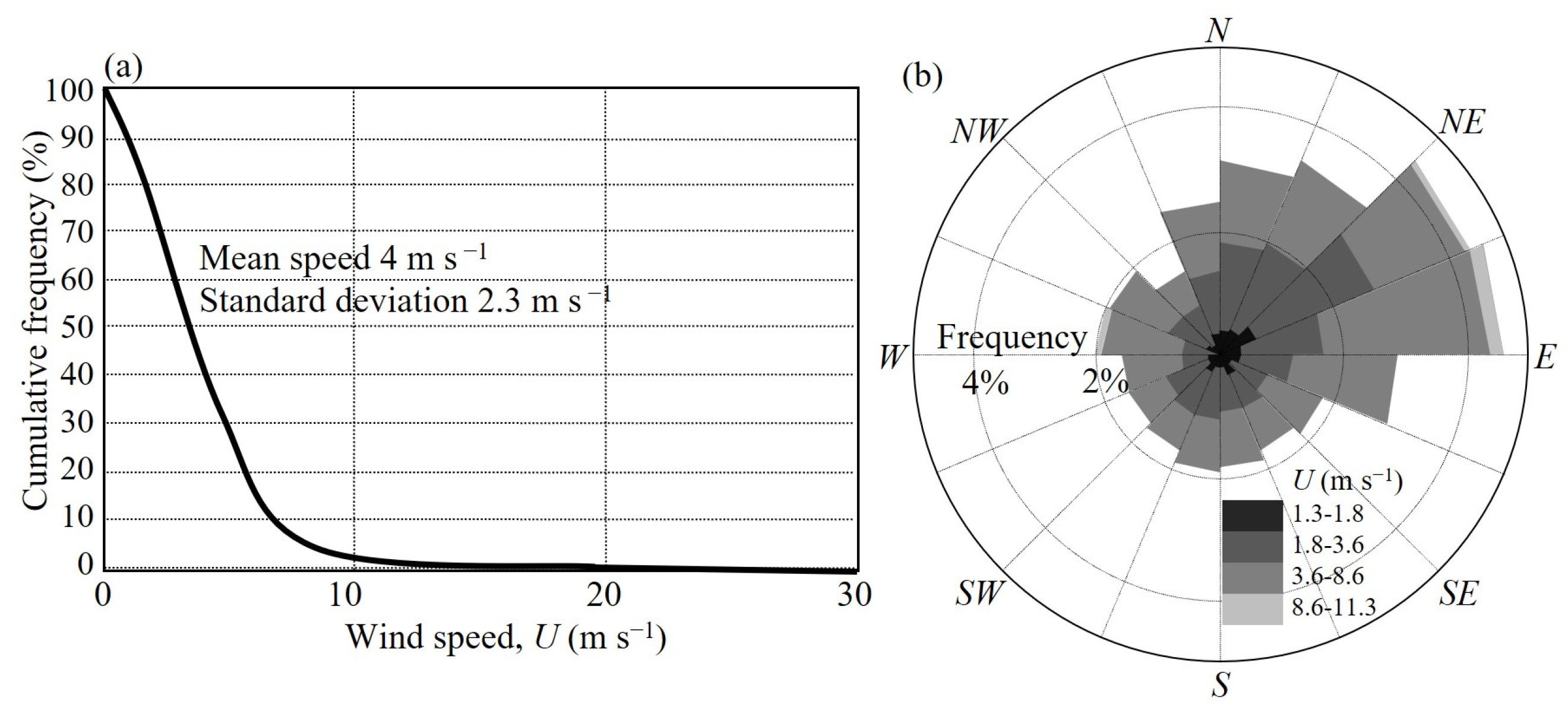
The distribution (percent) of wind speed U in Figure 2a is based on measurements at the tower (UF0) during the years 2002 to 2007. The mean speed was 4 m s⁻¹ with a standard deviation of 2.3 m s⁻¹. High winds were infrequent; the speed reached 30 m s⁻¹ only eleven times during those six years, which would mean a frequency of about two per year. An uncommon high value of 54 m s⁻¹ occurred in 2004 during the passage of Hurricane Jeanne across Central Florida. The wind rise for 2007 in Figure 2b indicates that northeasterly winds (in late fall and winter) are dominant. During the investigation, barring a single event when the wind reached 23 m s⁻¹, the maximum speed was less than 12 m s⁻¹, which made it essential to resort to modeling to estimate the SSC at higher winds.

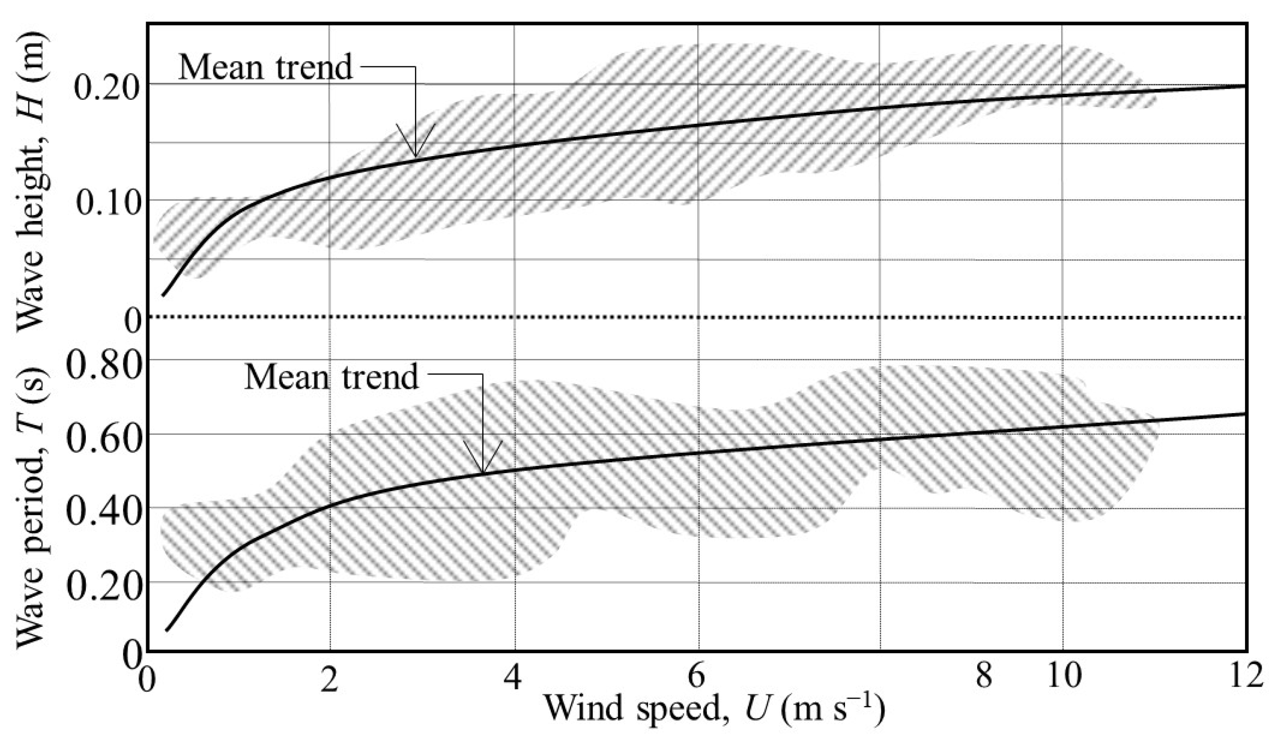
Figure 3 shows measurements (hatched areas) of the significant wave height H and period T. Although the typical wind direction was northeasterly, fluctuations in wind speed and duration (hence fetch) expectedly resulted in the observed data spread. Notwithstanding this limitation, the equation-based mean trends for wave height and wave period characteristically rise linearly in the low wind range, followed by decreasing rates of rise at higher winds [13].

Figure 4 plots a 27-day (starting January 2008) water level record and model simulation at UF0. Agreement is attested by the low error range of ±0.35% with a mean of 0.014%. The mean level was 19.4 m above the NAVD88 datum, which is equivalent to a mean water depth of 1.3 m. Low frequency (~2 × 10⁻⁶ Hz) frontal oscillations are significant, with the largest amplitude of 0.15 m amounting to ~12% of mean water depth. 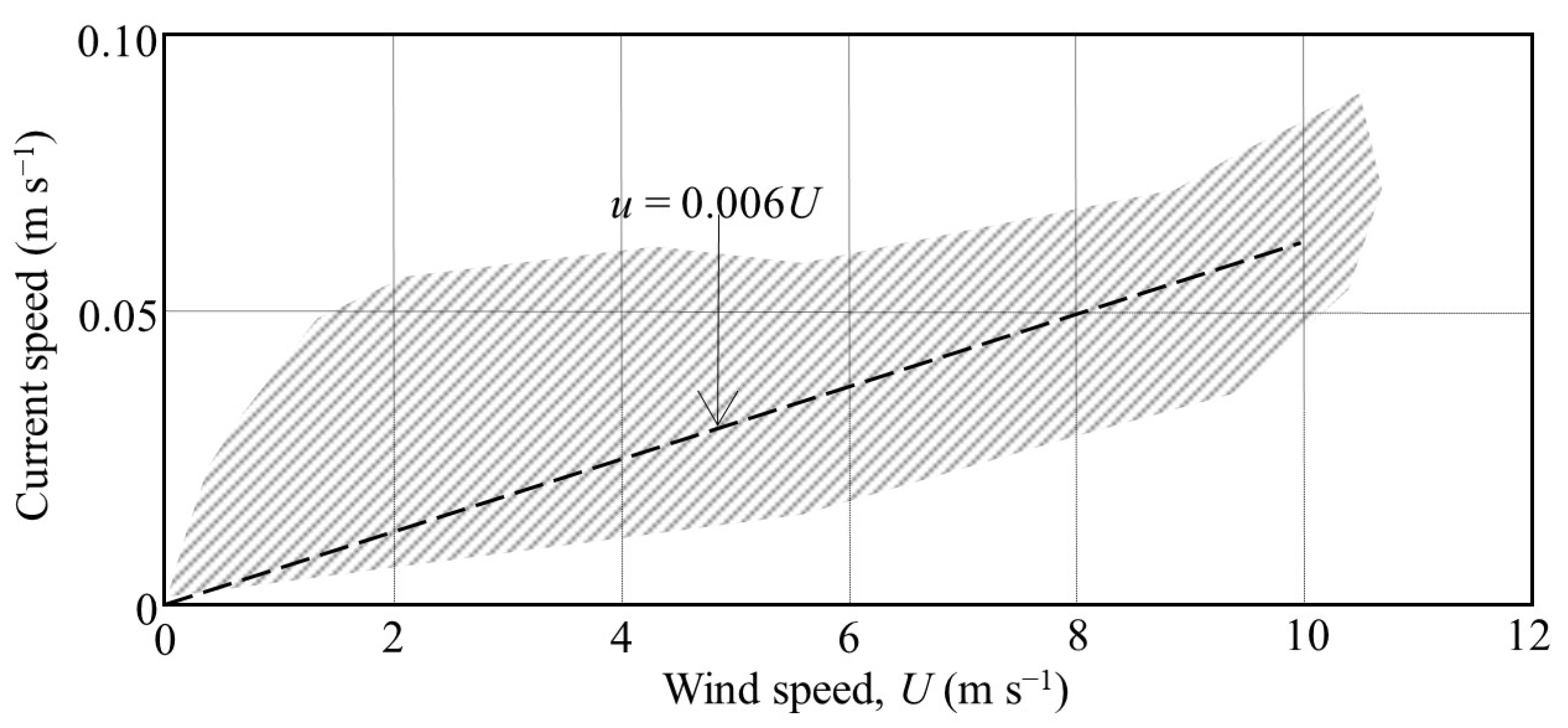Figure 5 shows the measured current vector u at the top of the BBL at 0.2 m elevation against wind speed. Temporal fluctuations in wind speed and direction, although generally aligned with the mean wave direction, are believed to be the cause of the data spread (hatched area). Dashed curve represents the model simulated mean trend. From simulations, the current at the surface u_s was found to be an order of magnitude greater than at 0.2 m, i.e., the coefficient 0.006 (inset) increased to 0.06, which is consistent with u_s resulting from wind-induced surface stress [14].

4. Suspended and Bottom Sediment

4.1. Layering and Density Profiles

Properties of the characteristically compressible flocs are conveniently defined by the floc volume fraction

$${\mathsf{\varphi }}_f={\displaystyle \frac{\Delta {\mathsf{\rho }}_s}{\Delta {\mathsf{\rho }}_f}}{\displaystyle \frac{C}{{\mathsf{\rho }}_s}}={\displaystyle \frac{\Delta {\mathsf{\rho }}_s}{\Delta {\mathsf{\rho }}_f}}\mathsf{\varphi }$$

(1)

where C is the sediment concentration as dry mass per unit volume of sediment plus water, ρ_s is the particle density, Δρ_s = ρ_s − ρ_w is the excess material density, ρ_w is the floc density, Δρ_f = ρ_f − ρ_w is the excess floc density, and ϕ = C/ρ_s is the particle volume fraction. Thus, the porosity is 1 − ϕ and the wet bulk density ρ = ϕΔρ_s + ρ_w.

Figure 6 schematizes the stratified density structure of the up to 2 m thick lake deposit defined by ϕ_f, which generally increases with depth. The threshold value ϕ_fh marks the transition between unhindered settling in the floc layer FL where ϕ_f < ϕ_fh and hindered settling in the fluid mud FM with ϕ_f > ϕ_fh. In FL, the floc settling velocity increases with increasing ϕ_f due to enhancement of the inter-particle collision frequency, while in FM the rate of settling is hindered due to increasing ϕ_f and decreasing inter-floc pore space. The suspension depth h is equivalent to the water depth. Under calm conditions in due course FM dewaters and changes into a soft stratified bed SB. Below the bed surface defined by ϕ_f = 1 (C = 54.3 kg m⁻³), settling occurs by consolidation of the interconnected particles. Due to its high organic content, the sediment has a low mean particle density ρ_s = 1873 kg m⁻³, with the inorganic component including kaolinitic particles and fine biogenic silica. The water density ρ_w in the lake is close to 1000 kg m⁻³, and the mean floc density ρ_f obtained from settling velocity and diameter measurements mentioned later is 1025 kg m⁻³.

Figure 7 illustrates the structure of the FL in the lake and as presently defined, the BBL above the bed, manifested by in situ instantaneous water salinity and temperature under practically calm wind condition using the temperature and salinity sensors of the Sea Bird transducer. The upper floc layer was largely composed of plankton and algae (top lab image) forming 150–300 μm macroflocs, i.e., with diameter > 100 μm. In the lower layer, flocs on the order of 1000–2000 μm with high porosity (≥0.95) were made of a translucent mucoid coating wrapped around a core (middle lab image), which typically was a mineral particle or plant matter. The BBL is separated from the lower floc layer by distinct peaks in salinity and temperature. They indicate a rapid decline both in salinity and temperature in the BBL, with high stratification suggesting a low rate of exchange of particulate matter between the FL and BBL. Moreover, biological decomposition in the expectedly somewhat anoxic BBL was likely low. The bottom, lab column-based image of slowly settling fluid mud reveals preferred paths facilitating the upward escape of water in the BBL when fluid mud is present. The thickness of the BBL is about 0.2 m, which was conveniently taken as the value applicable to the lake, although its local variability, or stability during high-wind events, was not investigated.

In Figure 8, ϕ_f profiles from two of the three cores show about 0.04 m of fluid mud above ϕ_fh of about 0.06 (estimated later and equivalent to C = 3.26 kg m⁻³), while in the third core the FM was absent. Mud in this state is believed to have occurred due to disturbances during the handling of the cores for density measurements. The top surface of the SB at ϕ_f = 1 (C = 54.3 kg m⁻³) expectedly coincides with the intersections of the three profiles. Below the surface ϕ_f increases above one, which, while indicating that it is no longer a fraction, remains a convenient measure of bed density. For all three cores, the SB and the uniform bed UB show similarity, suggesting that they were formed under comparable long-term hydrodynamic conditions. Over the thickness of the SB, ϕ_f increases rapidly with (negative) elevation z, having a mean rate of change of 0.11 m. In the UB, overburden from the SB and expected organic decomposition are believed to have resulted in material breakup and compression, due to which the maximum floc volume fraction ϕ_fm increased to about 1.8. In the MD, the effects of seasonal winds as well as sporadic efforts to eradicate the macrophytes, including the invasive Hydrilla, by herbicides [4] are believed to have led to a wide variability of ϕ_f between 1.8 and 2.8.

4.2. Significance of Rheometry

For the rheometric analysis, cores LTW-07, L05-07, L26-07, and L31-07 were sectioned into 3 to 4 cm segments, and a sample from each was tested in the viscometer. The inset of Figure 9a defines the shear stress (τ) vs. shear rate (G) flow curves of a shear-thinning pseudoplastic and, for comparison, its idealized Bingham plastic equivalent [15]. The quantity τ_y is the pseudoplastic yield strength, and η_∞ is the characteristic viscosity at a high (theoretically infinite) value of G. The plot indicates a characteristic pseudoplastic curve for the sample from core L31-07 with ϕ_f = 0.68 (C = 24 kg m⁻³). The τ_y of this sample was 0.03 Pa, and the η_∞ was 0.17 Pa s. Overall, η_∞ values from all four cores were found to be insensitive to ϕ_f, ranging between 0.15 and 0.20 Pa s with a mean close to 0.17 Pa s (as in Figure 9a), which is two orders of magnitude greater than water.

Figure 9b is a plot of τ_y against ϕ_f. Values of ϕ_f, both lower and higher than one, indicate that the samples included mud as a fluid and as a soft bed. The high power (4.35) of the mean trend implies a rapid increase in inter-particle electrochemical and biochemical bonding with increasing ϕ_f. Note that τ_y extrapolated to ϕ_fh = 0.06 (C = 3.26 kg m⁻³), i.e., at the transition between fluid mud and the more dilute flocculated suspension, is practically nil (<<0.01 Pa). At the bed surface (ϕ_f = 1), the τ_y of about 0.10 Pa equals the bed shear stress τ_b at which stress-induced reworking of the bed can be expected to commence, and as τ_b exceeds 0.10 Pa the thickness Δh of the reworked bed increases [16]. Derivative evidence of reworking is apparent from profiles of the radioactive tracer ⁷Be (Beryllium-7 and a half-life of 53 days) obtained from the upper 0.10 m of the cores. ⁷Be is supplied from the atmosphere and is often used to track fine sediment resuspension, with its radioactivity acceptable as a proxy for Δh within the decay timescale of the tracer [17]. In Figure 10, which shows the ⁷Be profile from the core LTW-07, complete mixing occurred up to the depth of 0.03 m; below that level it was partial and was nil in the deeper layers. As mixing can be mechanical and by bioturbation, there is a likelihood that diffusion of ⁷Be below 0.03 m was both physically and biomechanically induced, possibly by benthic invertebrates in the BBL [18].

Combining the trend of variation of ϕ_f with z in the top 0.10 m of the SB in Figure 8, the variation of τ_y with ϕ_f in Figure 9b, and equating τ_y to the wind-applied bed shear stress τ_b, we obtain

$$\Delta h=0.11(1-1.76{\mathsf{\tau }}_b^{0.23})$$

(2)

in which, at the depth Δh, τ_b = τ_y. Values of Δh ranging between <0.01 m and 0.03 m from replicate cores at the four sites are given in

Table 2. Estimates of reworked bed thickness.

Core	Reworked Bed Thickness, Δh (m)
LTW-07A	0.030
L05-07A	<0.01
L26-07A	0.030
L31-07A	<0.01
LTW-08A	0.013
L05-08A	0.013
L26-08A	0.013
L31-08A	0.023

. Taking 0.013 m as a representative value, from Equation (2) the corresponding τ_b would be 0.14 Pa, which can be shown from the modeling to be equivalent to a wind speed of 11–12 m s⁻¹, which occurred on occasions. Thus, the rough calculation suggests that bed reworking took place over timescales shorter than the time for tracer decay, i.e., over a month or two prior to sampling. The low frequency of bed weakening and the bed shear strength may also be a partial cause why fluid mud generally does not flow over bed slopes in the lake, thereby preserving its uneven bathymetry (Figure 1b).

5. Resuspension Dynamics

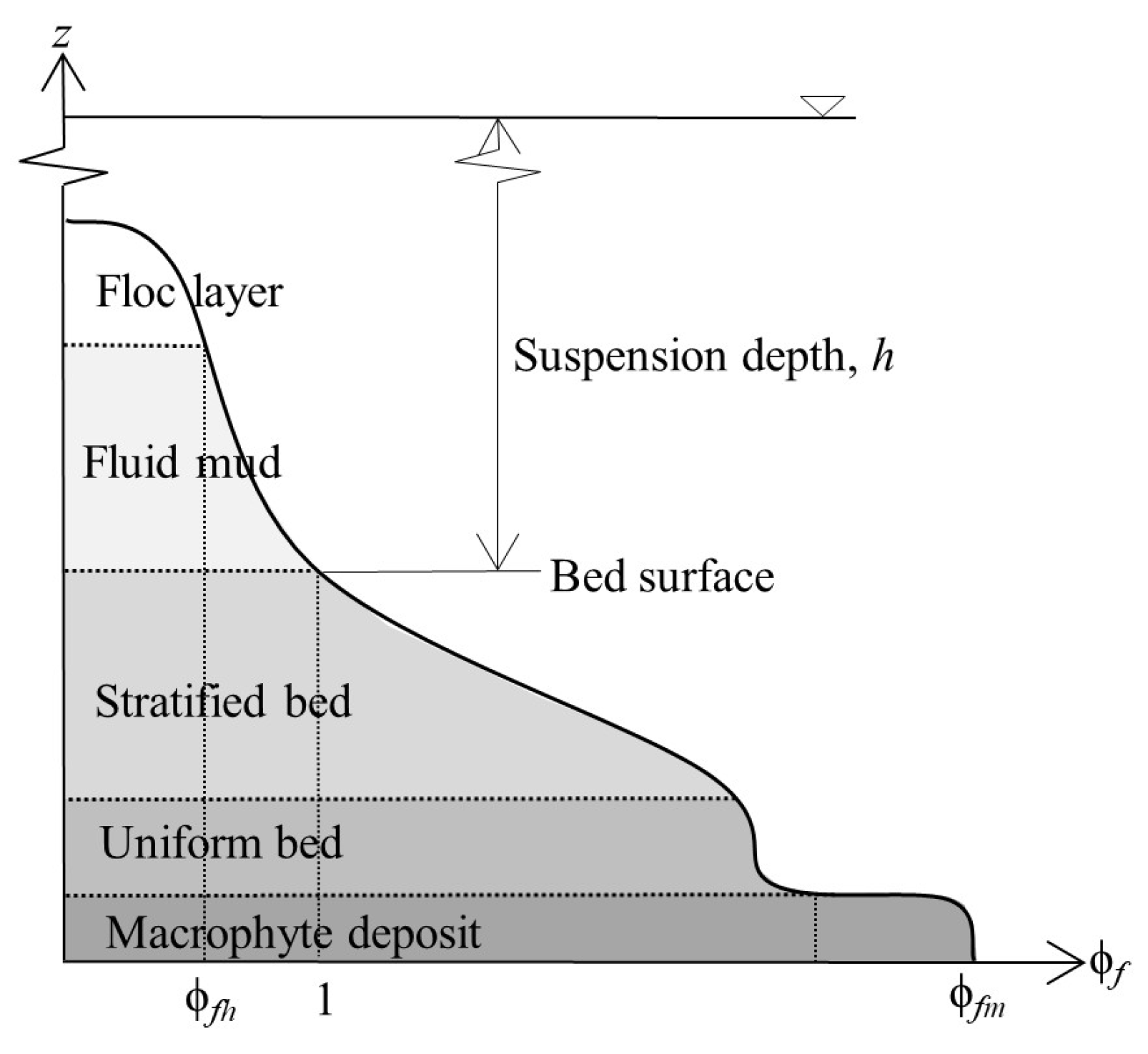
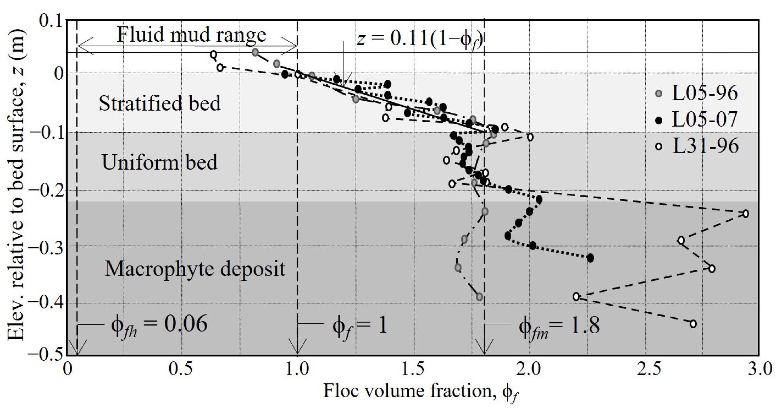
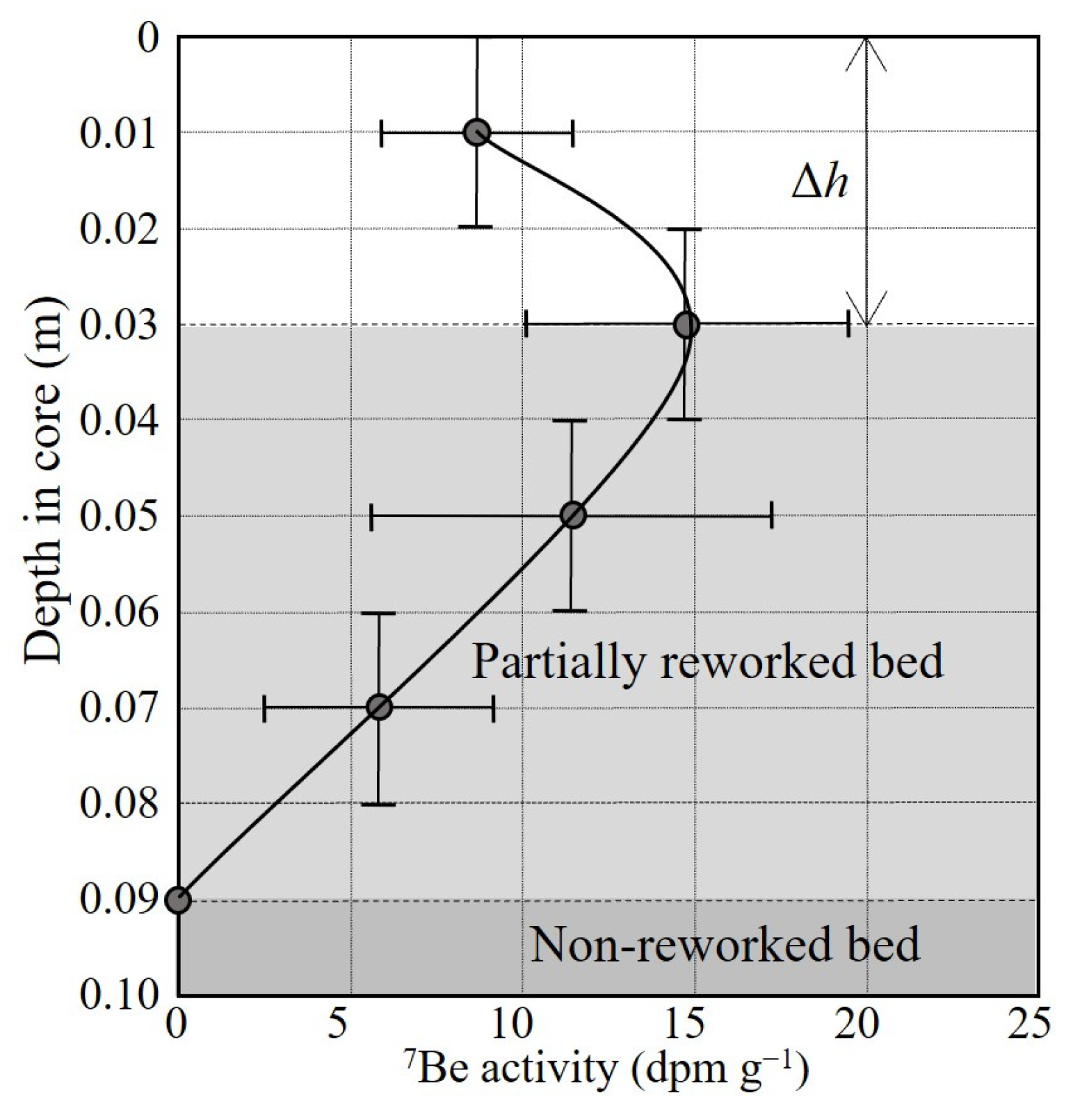
During a high-wind episode, fluid mud occurs in the BBL when the bed sediment erodes and rises upward by turbulent diffusion and at the end of the episode when the suspension begins to settle relatively rapidly at the onset and stacks up above the bed as fluid mud, which then settles slowly. The timescales for both erosion and settling in Lake Apopka are the order of an hour. Presently, we will focus attention on the rising phase of the fluid mud, with significant fluid mud considered to occur when its height Δh_F reaches the top of BBL (at 0.2 m) as ϕ_f increases to ϕ_fh at that elevation. In this condition, ϕ_f below 0.2 m characteristically increases above ϕ_fh with depth.

For modeling erosion and settling, the deposition flux D_r in the suspended sediment mass balance in each model grid cell is

$$D_r={\mathsf{\rho }}_s{\mathsf{\varphi }}_f{w}_f({\mathsf{\varphi }}_f,G)$$

(3)

where the floc settling velocity w_f is a function of ϕ_f and the shear rate G. The bed surface erosion flux E_r is

$$E_r=f({\mathsf{\tau }}_b,{\mathsf{\tau }}_e)$$

(4)

where f(τ_b, τ_e) denotes a function of the wave-current bed shear τ_b and the erosion threshold stress τ_e. The former was calculated from

$${\mathsf{\tau }}_b=\mathsf{\chi }\left({\mathsf{\tau }}_{bw}+{\mathsf{\tau }}_{bc}\right)$$

(5)

where τ_bw and τ_bc are the wave- and current-induced bed shear stresses, respectively, and χ is a proportionality coefficient. At any grid cell defined by the local depth, to calculate τ_b from Equation (5) for a given wind speed and fetch, the wave height and the period at that cell were determined first. The stress τ_bw was obtained from the near-bed, linear-wave orbital velocity with a drag coefficient based on k_s = 0.065 m [13]. The stress τ_bc was calculated from the model-simulated hydrostatic current velocity in the bottom-most layer, which includes inherent contributions from wind-induced water level setup in the lake, and χ was obtained from a method provided by [19].

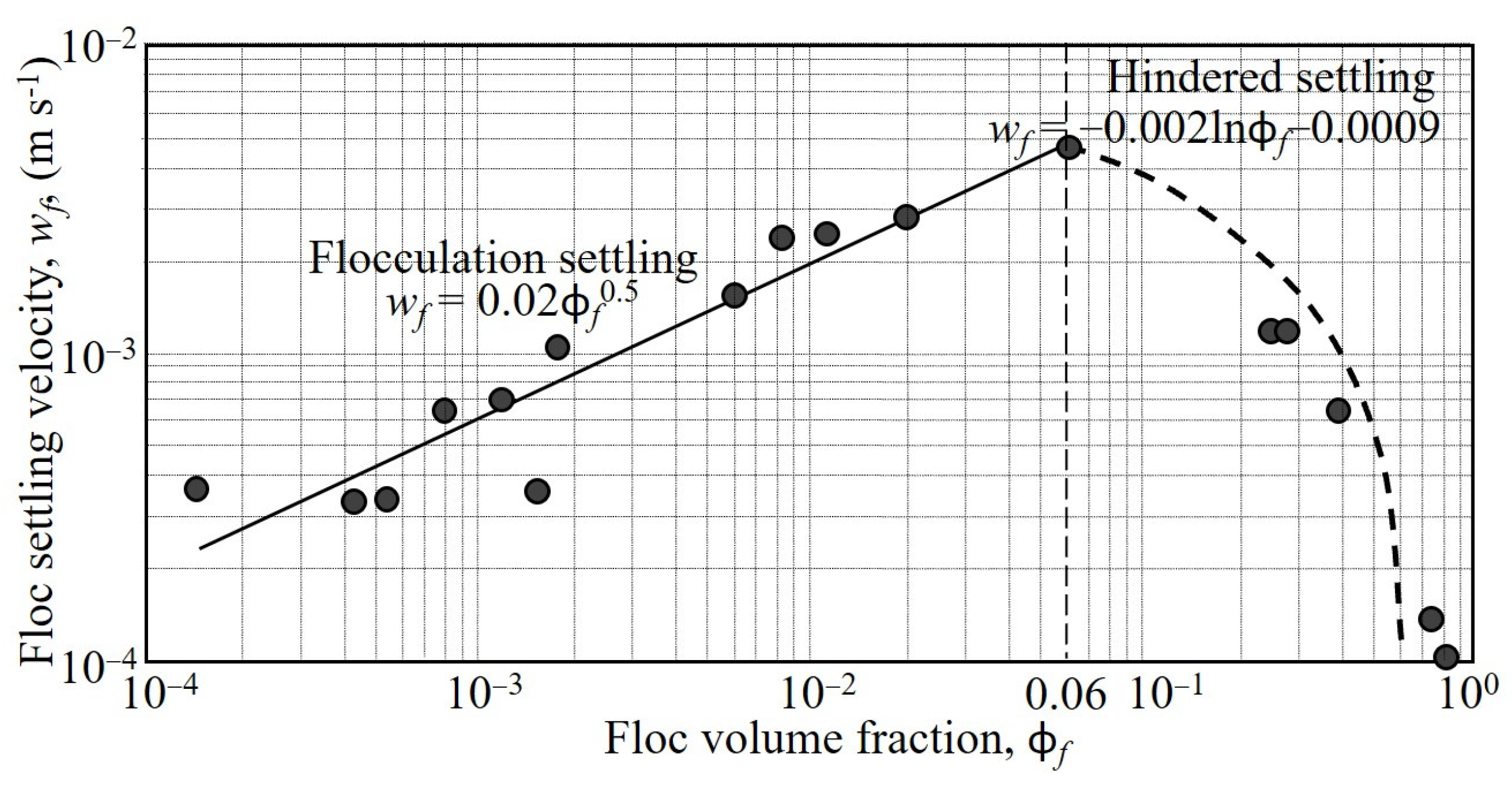
The settling velocity w_f was evaluated from on-site tests in a 1 m tall column using suspended sediment samples collected near UF0, and w_f at higher ϕ_f were obtained from a 1.85 m tall laboratory column [20]. The plot of w_f against ϕ_f in Figure 11 identifies ϕ_fh as 0.06 (3.26 kg m⁻³), which is typical for organic-rich fine sediments but lower by about a half than clay mineral flocs [10]. Due to the low currents under normal conditions in the lake, the roughness Reynolds number Re_f = k_s(ρ_wτ_b)^0.5/η_w is below 500, implying that both skin friction and form drag contribute to the turbulent energy loss. Given low Re_f and assuming that the role of shear rate G is minor, data fits yield the approximate formulas for unhindered (flocculation) and hindered settling given in the inset in Figure 11.

Due to inter-particle cohesive bonding in the stratified bed SB manifested by the effective normal stress, bed compression from consolidation is characteristically slow compared to hindered settling. To confirm this, measurements of the falling sediment/water interface were made in the 1.85 m column, starting with an initial floc volume fraction ϕ_f0 = 1.07 (C₀ = 58.1 kg m⁻³) and a deposit height of 0.45 m [20]. It was observed that the time to decrease the height of the bed to 0.22 m (thus doubling the depth-mean ϕ_f) was about 17 h, i.e., a mean settling rate of 6.4 × 10⁻⁸ m s⁻¹. Based on this duration relative to the hindered settling velocity on the order of 10⁻⁴ m s⁻¹ (Figure 11), consolidation was assumed negligible in modeling resuspension.

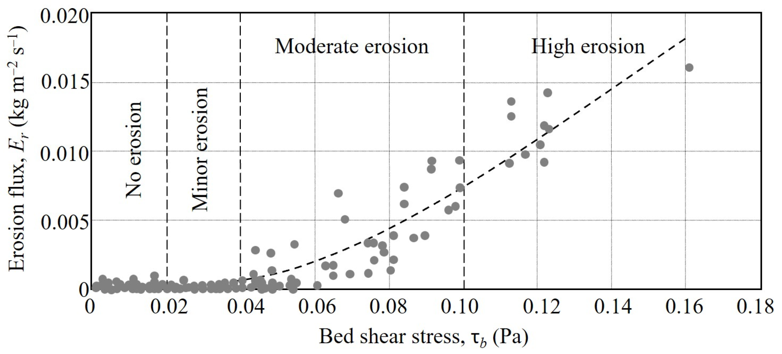
The variation of bed surface erosion flux E_r with τ_b in Figure 12 is based on SSC measurements at UF0 augmented by available synchronous data from UF1 and UF2. The following polynomial equation [21], whose basis is a stochastic treatment of erosion by the turbulent, time-dependent bed shear stress, was used to generate the mean trend

$$f({\mathsf{\tau }}_b,{\mathsf{\tau }}_e)={\mathsf{\tau }}_e\left[a_1{\left({\displaystyle \frac{{\mathsf{\tau }}_b}{{\mathsf{\tau }}_e}}\right)}^3+a_2{\left({\displaystyle \frac{{\mathsf{\tau }}_b}{{\mathsf{\tau }}_e}}\right)}^2+a_3\left({\displaystyle \frac{{\mathsf{\tau }}_b}{{\mathsf{\tau }}_e}}\right)+a_4\left({\displaystyle \frac{{\mathsf{\tau }}_b}{{\mathsf{\tau }}_e}}-1\right)\right]$$

(6)

with τ_e = 0.02 Pa, a₁ = −190.03, a₂ = 83.57, a₃ = −2.99, and a₄ = −0.02. The curve generally represents the data up to τ_b = 0.12 Pa but is somewhat speculative at higher stresses due to the scarcity of measurements. Notwithstanding this constraint, the trend is conveniently divided into four zones—no erosion (τ_b < 0.02 Pa), minor erosion (0.02 Pa ≤ τ_b < 0.04 Pa), moderate erosion (0.04 Pa ≤ τ_b < 0.10 Pa), and high erosion (τ_b ≥ 0.10 Pa). The threshold 0.10 Pa coincides with the onset of bed weakening. However, as its effect on surface erosion cannot be readily quantified, Equation (6) is assumed to apply over the full range of τ_b.

6. Fluid Mud Dynamics

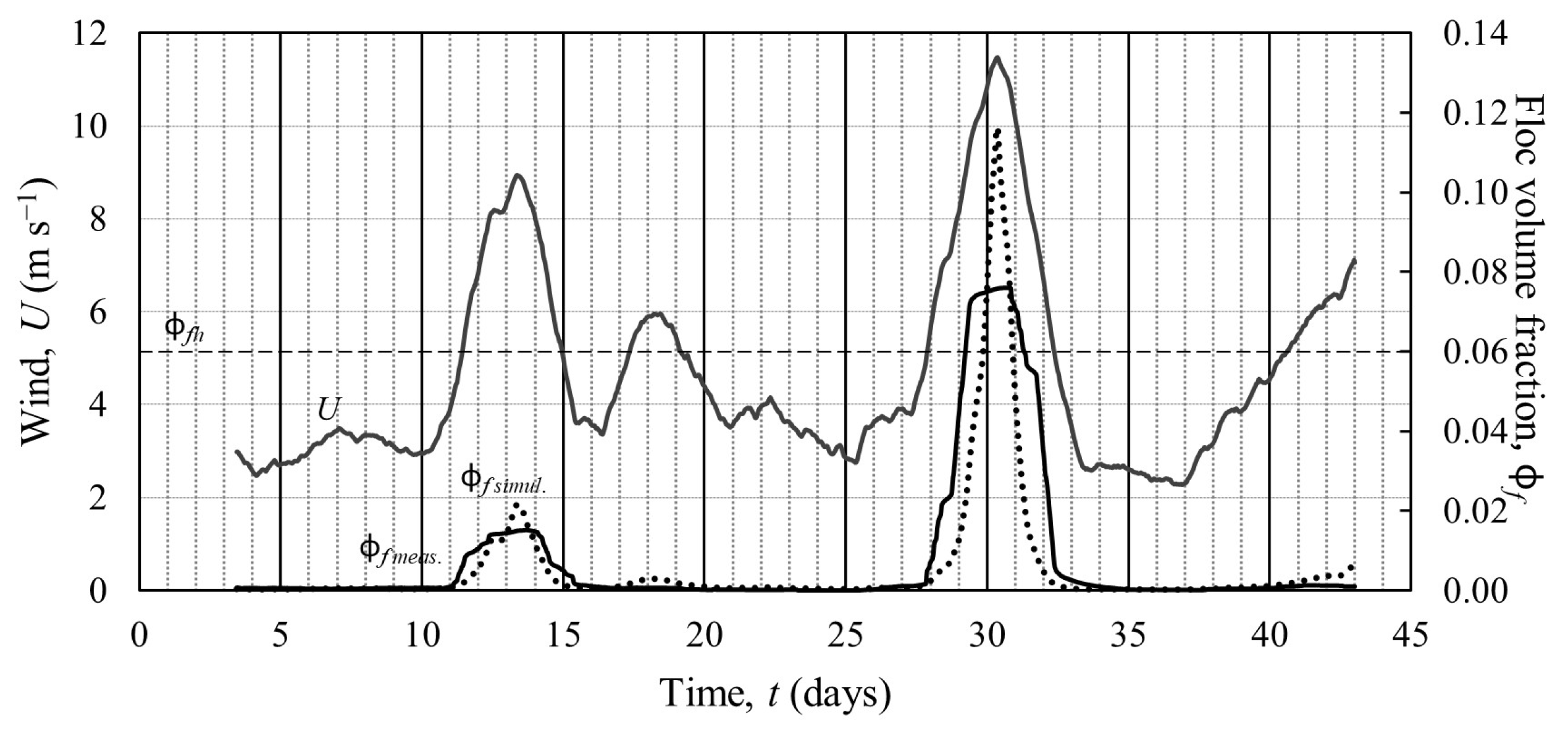
Figure 13 plots ϕ_f against wind speed at UF0 over a 41-day period beginning 9 December 2007. Two significant episodes separated by relatively calm weather over about ten days have been captured, although, typically, the maximum wind remained less than 12 m s⁻¹. The measured floc volume fraction ϕ_fmeas is generally synchronous with the wind, having a correlation coefficient of 0.78. The inference would be that wave-induced local erosion and deposition, as opposed to weak current-induced advection, largely govern the variation of SSC. This is supported by the simulated floc volume fraction ϕ_fsimul, which correlates well with the wind (correlation coefficient of 0.91). Moreover, ϕ_fmeas and ϕ_fsimul indicate a correlation coefficient of 0.86 and a reasonably low mean error of 26%. Observe that fluid mud rose to the height of the BBL just once, on days 29–30, when the wind peaked at 11.6 m s⁻¹.

To illustrate the rise of fluid mud due to erosion, Figure 14a shows simulated ϕ_f profiles at UF0 after 1 h of wind ranging from 5 to 23 m s⁻¹. As with the Rouse equilibrium condition [22], these profiles exhibit a monotonic increase in ϕ_f with depth. Fluid mud rises just above the top of BBL (at 0.20 m with ϕ_f = 0.06) when the speed exceeds 10 m s⁻¹. The profiles indicate that an overwhelming amount of particulate mass is contained in the BBL relative to the upper floc layer. For U ranging from 5 to 23 m s⁻¹, the ratio (percent) of mass in the upper layer to that in BBL varies from 0.02 to 1.3%. Figure 14b indicates that measurements and simulation of ϕ_f reasonably concur at lower winds, which supports the model’s ability to predict ϕ_f at high winds.

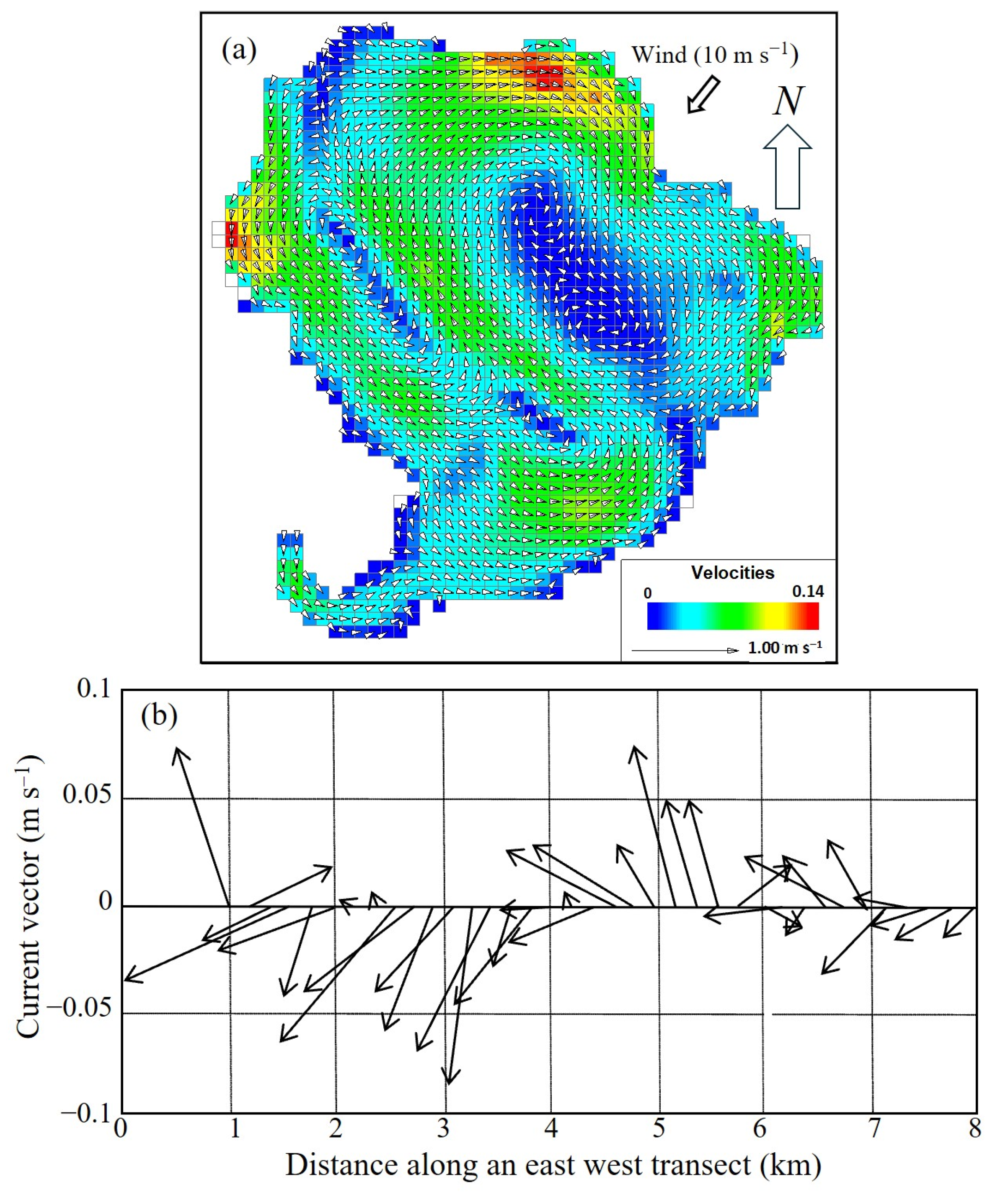
Even a steady wind generates an intertwined circulation pattern as seen in Figure 15a showing modeled depth-mean hydrostatic current velocity vectors in 1.3 m mean depth of water and a northeasterly wind of 10 m s⁻¹ blowing for an hour. As expected, the blue zones of lowest currents (<0.02 m s⁻¹) are found in deeper waters (Figure 1b), whereas the highest currents (>0.1 m s⁻¹) are along the lake’s shallow periphery. The largest (anticyclonic) eddy roughly scales with the lake, midscale eddies, are a few kilometers in diameter, and identifiable small eddies are 1–3 km. Shear zones, which tend to promote lateral exchange of water, are apparent at the confluent flow boundaries.

Figure 15b is based on underway measurements using an ADCP at a depth of about 0.5 m below the water surface from a small shallow draft vessel moving at a mean speed of 1.2 m s⁻¹. The single westward run was made on 1 November 2007, along the trajectory shown in Figure 1b when the dominant wind was northeasterly at a speed of about 9 m s⁻¹. Qualitative agreement between the current velocity vectors with the simulated eddies in Figure 15a is suggested from the directional pattern of the vectors with distance and that the measured velocities were associated with smaller eddies.

Tropical storms are anecdotally known to cause high turbidity in the lake [23]. At 23 m s⁻¹ northeasterly wind, simulated depth-mean currents are shown in Figure 16a and the respective floc volume fraction pattern in Figure 16b. The estimated wave height at UF0 was 0.25 m, and the period was 0.85 s. Circulation is dominated by two or three large eddies and markedly differs from the pattern at 10 m s⁻¹ (Figure 15a) illustrating the high dependence of circulation on wind. The ϕ_f contours expectedly conform in a general sense with the flow pattern. Fluid mud (ϕ_f ≥ 0.06) is found throughout, except in the lower tail of the lake at Gourd’s Neck.

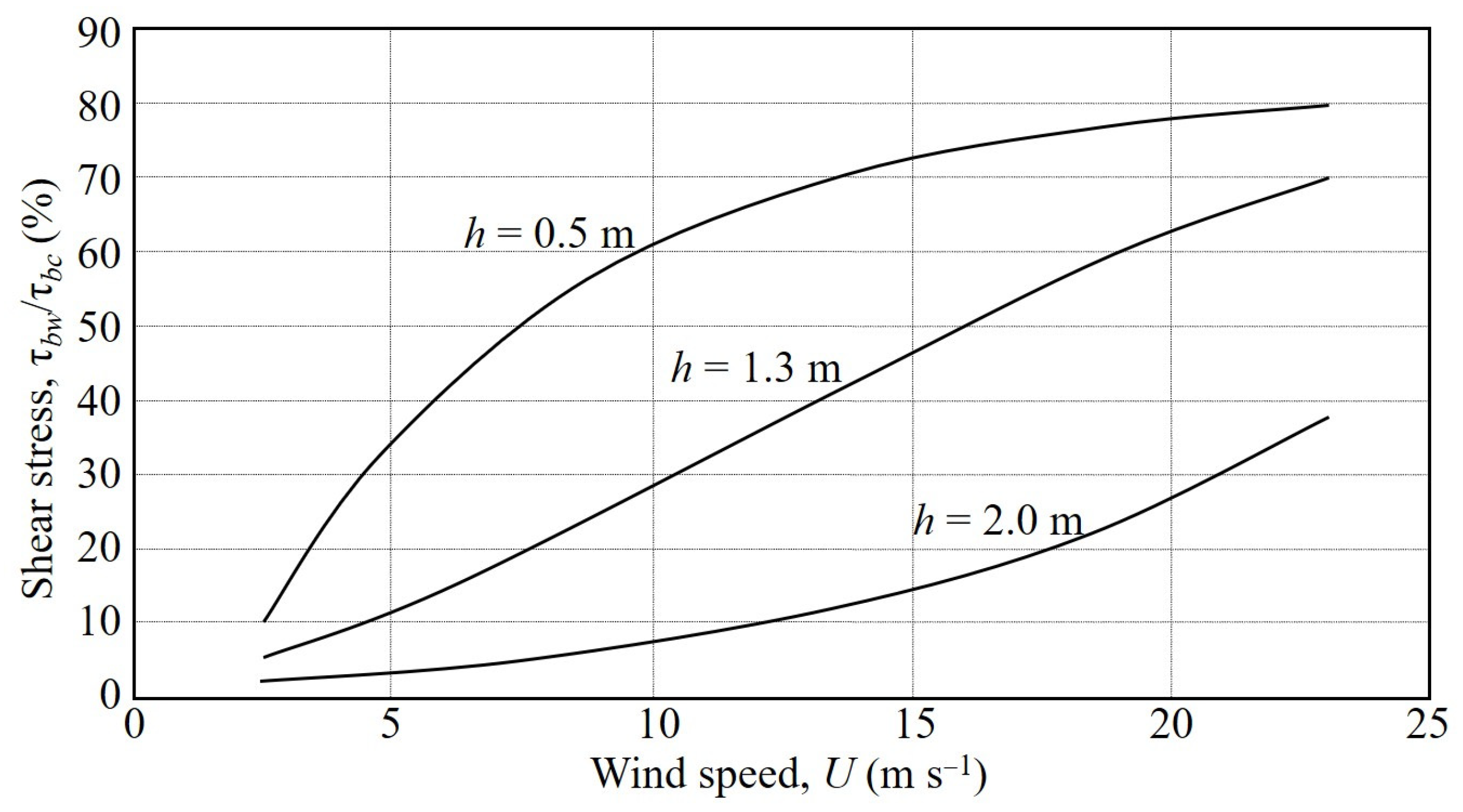
7. Effect of Water Depth

As a measure of the relative roles of waves and currents at different water depths, model-calculated ratio of wave bed shear stress to current bed shear stress τ_bw/τ_bc (%) is plotted in Figure 17 as a function of wind speed U and water depth h. As h increases, the effects of both U and h on the bed shear stress expectedly decrease, and wave influence decreases (τ_bw) relative to current (τ_bc). In shallower water (0.5 m), waves have a measurable impact comparable to currents when U increases to ~10 m s⁻¹ (τ_bw/τ_bc = 61%). At 1.3 m mean depth, waves begin to have a comparable role when U exceeds ~15 m s⁻¹ (τ_bw/τ_bc = 47%). In 2 m deep water, the role of waves is low compared to the current until U is very strong, e.g., τ_bw/τ_bc = 32% at a high 23 m s⁻¹. These changes imply that, apart from fluid mud, variability in the wave-current boundary layer, including τ_b, with wind speed and water depth plays a role in BBL dynamics with a potential impact on the biota.

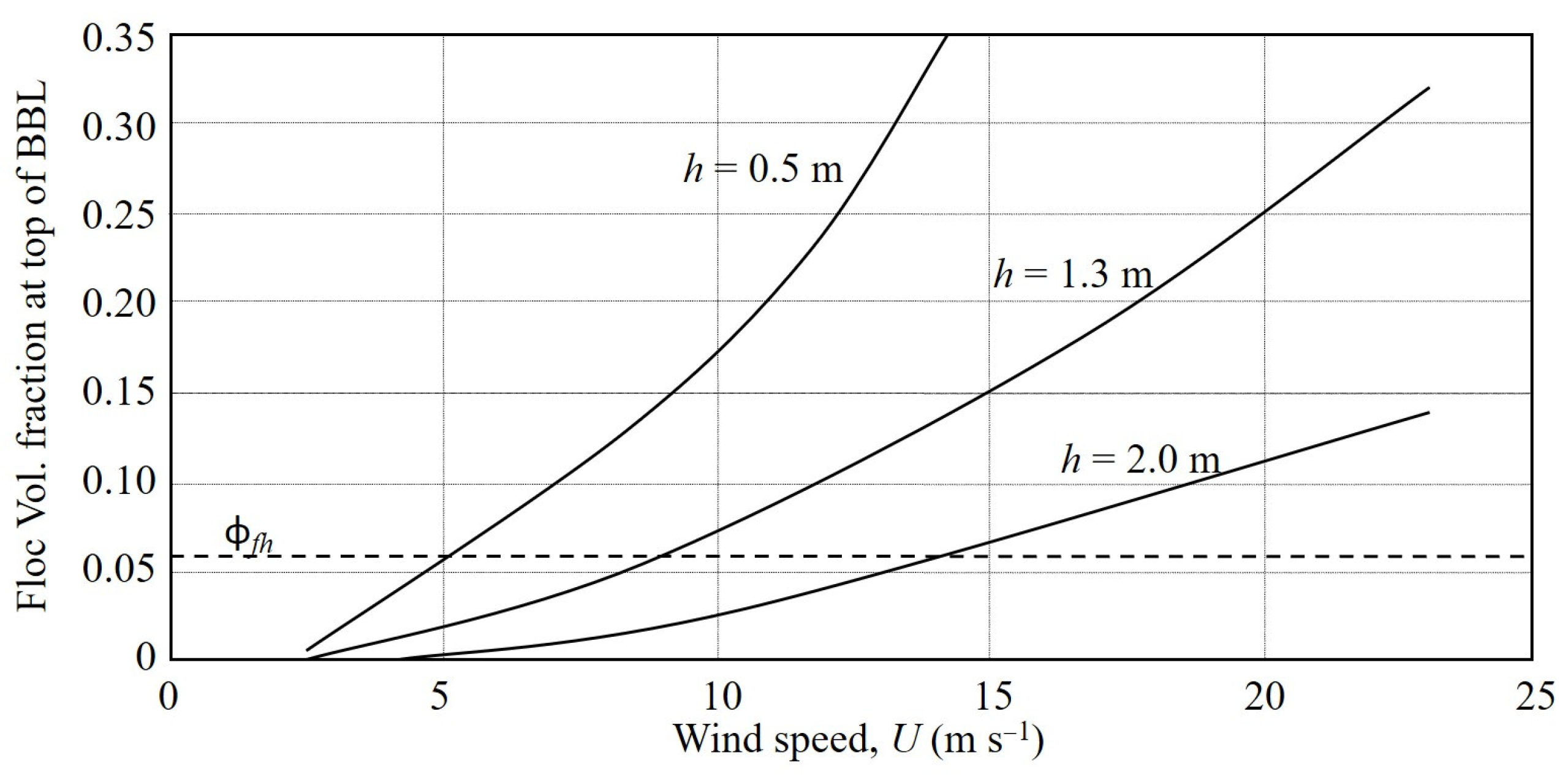
In Figure 18, simulated floc volume fraction curves at the top of BBL are shown at different wind speeds and the selected water depths. Expectedly, the effect of changing the depth is significant; for instance, at a wind of 10 m s⁻¹ in 2 m deep water ϕ_f = 0.024 (C = 1.3 kg m⁻³), whereas in 0.5 m depth it is 0.18 (C = 9.8 kg m⁻³), which amounts to a 7.5-fold increase in the SSC.

Referring to Figure 17 and Figure 18, both field and lab measurements have characteristic uncertainties, with the largest error likely to be in the SSC time series, which essentially are single-point values conditioned by the local hydrodynamics. Relative to modeling, the accuracy of wave-current bed shear stress is limited by use of simple wave prediction equations. In general, from a rough estimation it is concluded that, while the uncertainty in the calculated stress ratio (Figure 17) and the volume fraction (Figure 17) increase with wind speed, the overall mean errors are less than 20%. To minimize these in future, three improvements in measurement and modeling are recommended: (1) Make the SSC time-series measurements within the BBL, (2) incorporate an advanced model for wave prediction, and (3) further validate the trends in Figure 17 and Figure 18 by model testing against measurements at wind speeds higher than 12 m s⁻¹. The last improvement is unquestionably most important, as it would reduce exclusive reliance on modeling for the prediction of BBL height at high winds.

8. Concluding Comments

To provide an understanding of the role of water level in the probability of wind-induced rise of fluid mud, this work proposes a field-based and modeling protocol generic enough to be applied to other lakes with similar management issues. As fluid mud dynamics are specific to the lake depending on the local climate, physiography, and fine sediment properties, the method must be calibrated against experimental data akin to those collected in the present study.

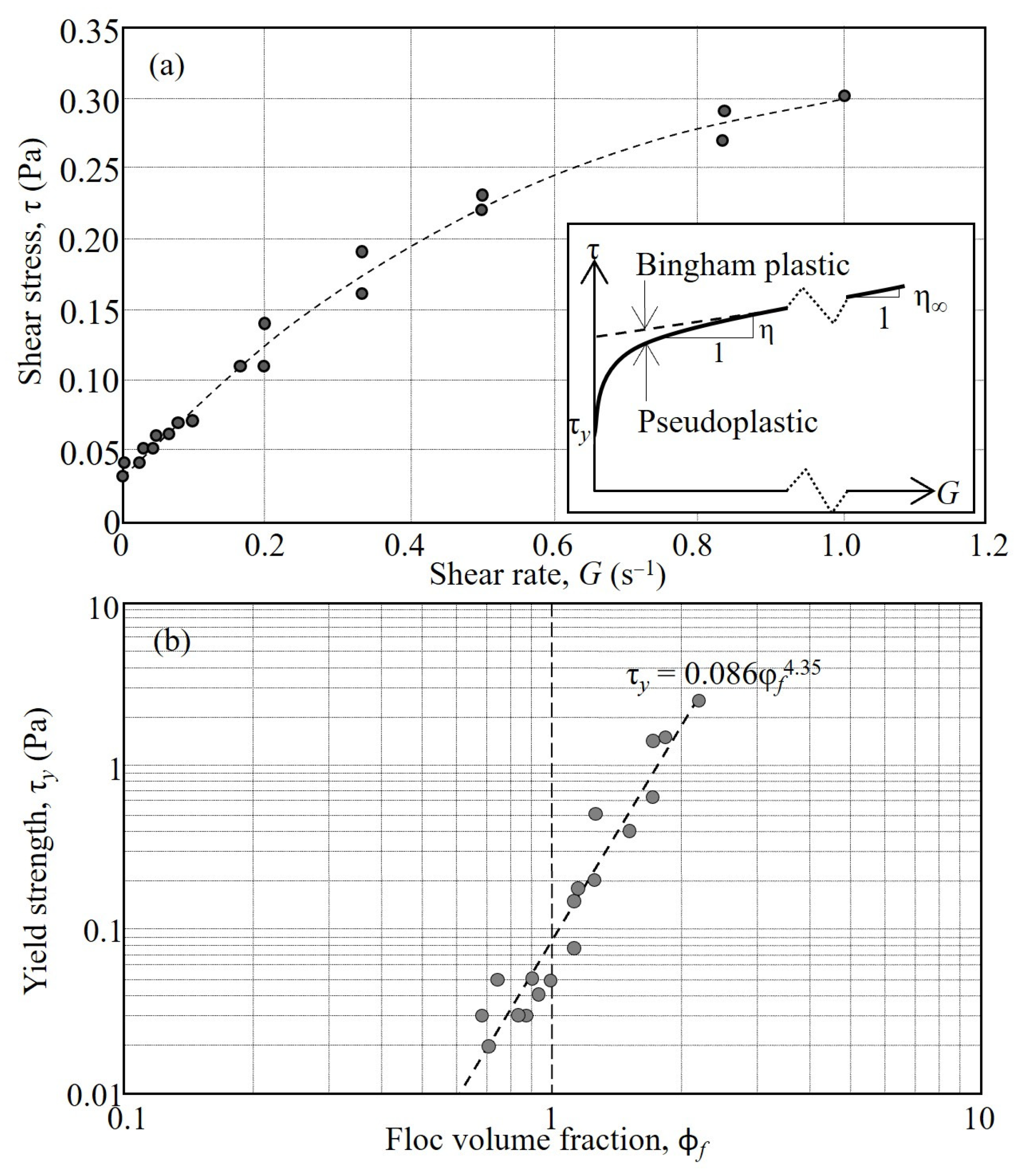
Three notable features of Lake Apopka are the shallow depths, organic-rich flocculated sediment, and resuspension governed by episodic wind. Under these conditions, the presence of fluid mud in the BBL influences the lake in at least two likely ways. Firstly, with its high viscosity (0.17 Pa s), fluid mud tends to absorb wind-induced energy at a much greater rate than water, thereby dampening turbulence. For instance, at a shear rate G = 1 s⁻¹ the rate of wave energy dissipation in water would be 10⁻⁶ m² s⁻³, whereas at the same G in fluid mud it would increase a hundred-fold to 1.7 × 10⁻⁴ m² s⁻³ [24]. Thus, for example, when there is a long-term increase or decrease in SSC, aquatic life can be affected in major ways, because both nutrient recycling and habitat suitability for benthos are altered [25,26,27].

Secondly, fluid mud influences the rates of the fall and rise of SSC. Consider a non-hindered settling suspension at ϕ_f = 0.01 (C = 0.54 kg m⁻³), which settles in the flocculation settling mode compared to one at, for illustration, a high value of ϕ_f = 0.6 (C = 32.6 kg m⁻³), which would settle in the hindered mode. From Figure 11, the respective settling velocities would be approximately 0.002 m s⁻¹ and 0.0002 m s⁻¹. Considering the suspension to notionally remain uniform, the times for the suspension/water interface to settle over a height of, say, 0.2 m would be 40 s and 2000 s, respectively. A potential consequence of the slow settling of fluid mud with characteristically low shear strength would be that if, for instance, a second wind episode were to occur while the fluid mud was settling, turbidity rise from its re-entrainment would be far more rapid than if the fluid mud had reverted to a more resistant bed.

A noteworthy experimental effort was made by the construction of a wetland for phosphate removal in the lake between November 2003 and March 2007. It showed a consistent annual reduction in the total phosphorus [28]. Given the interaction of fluid mud with biota and the need to further consider solutions for water quality improvement, the complex dynamics of the BBL requires a more detailed investigation, especially at high winds. In general, notwithstanding the hiatus in our understanding of BBL dynamics, our preliminary main conclusion is that at the normal water depth of 1.3 m, fluid mud occupies the BBL when the threshold wind exceeds about 9 m s⁻¹ corresponding to a 4% probability of occurrence, whereas at 2 m depth the threshold would be about 14 m s⁻¹ with a low probability of 2%. Thus, provided a water depth greater than 1.3 m can be sustained in the large lake, the deduced relationship between fluid mud rise, wind speed, and mean water depth makes it feasible to select the depth at which the rise of fluid mud in the BBL has an acceptably low probability.

While calculating the cost of maintaining a comparatively high-water level in the lake is beyond the present scope, it is understood to be more economical than, for instance, dredging out the accumulated fine sediment, which is not independent of the cost of disposal of the contaminated material.