The Seasonal Correlation Between El Niño and Southern Oscillation Events and Sea Surface Temperature Anomalies in the South China Sea from 1958 to 2024

Abstract

This study utilizes high-resolution sea surface temperature (SST) reanalysis data (0.25° × 0.25°) to investigate the relationship between SST anomalies in the South China Sea and ENSO events. The main findings are as follows: First, there is a delayed correlation between ENSO and SST anomalies in the South China Sea, with the correlation being stronger during El Niño years than during La Niña years. Second, the correlation with the peak values of the Oceanic Niño Index (ONI) is strongest for El Niño events with a 9-month lead, while for La Niña events, it is strongest with a 2-month lead. Seasonally, during El Niño events, the strongest correlations are observed in summer with a 3-month lead and in winter with a 1-month lag. For La Niña events, the strongest correlations are seen in summer with an 8-month lag and in winter with a 9-month lag. Finally, an analysis of atmospheric anomalies and shear kinetic energy anomalies relative to SST anomalies reveals a significant seasonal SST response, particularly during the summer of El Niño years and the winter of La Niña years. Overall, these results enhance our understanding of ENSO’s influence on the South China Sea and provide valuable insights for climate prediction and ecosystem protection in the region.

1. Introduction

El Niño and the Southern Oscillation (ENSO) constitute the principal climate phenomena that exert an influence on interdecadal climate variability on a global scale [1]. ENSO events are typically regarded as self-sustaining oscillations or responses to external forcing within the ocean–atmosphere system [2]. The impacts of ENSO extend globally, particularly through remote teleconnections [3]. Recent research has placed emphasis on the increasingly close link between ENSO and sea surface temperature (SST) in the tropical south Atlantic, which has an impact on rainfall patterns in South Asia [4]. Similarly, tropical Indian Ocean SST warmed in response to ENSO-related Pacific warming, lagging by two seasons [5]. Atlantic warming occurred several months after the peak of Pacific warming [6]. In the South China Sea, SST anomalies (SSTA) are associated with ENSO events and typically reach their peak 5–6 months after the event [7,8]. During the mature phase of ENSO and the subsequent summer, sea temperatures in the region are conspicuously warmer, especially in winter and the subsequent summer [9,10]. These changes are driven by atmospheric circulation and monsoon variability [11], and the seasonal distribution of sea temperatures is also influenced by the seasonal cycle and ground circulation [12]. An analysis of sea temperatures in the second half of the 20th century reveals that El Niño events in the eastern Pacific have an average duration of 15 months, and in the central Pacific, an average duration of 8 months [1]. In recent decades, El Niño events have increased, characterized by the highest sea temperatures in the equatorial Pacific central region [13]. The influence of ENSO on the evolution of sea temperatures in the equatorial Atlantic also demonstrates significant multidecadal variability [14]. During El Niño events, alterations in atmospheric circulation modify local surface conditions (temperature, humidity, cloud cover, and monsoon patterns), affecting heat fluxes and currents and thereby sea temperatures. In the South China Sea, sea temperatures and ENSO events lag by 5 months [15,16]. Furthermore, ENSO-related large-scale sea temperature variability in the Indian Ocean is associated with anomalies in net heat fluxes. It is highlighted that in the summer, El Niño and La Niña events cause asymmetric intensities of weather disturbances in the western North Pacific [17]. The South China Sea is located at the intersection of the Asian continent, the Indian Ocean, and the Pacific Ocean, and is a key region for the South China Sea monsoon and an important water vapor channel influencing East Asian weather and climate [11]. Its sensitivity to changes in the East Asian monsoon and West Pacific conditions is well documented [18]. Previous studies have mainly focused on the interdecadal variability of sea surface temperature in the South China Sea, and recent research has emphasized the seasonal-scale correlation and significant impact of El Niño and La Niña on regional precipitation variability. For instance, spring ENSO teleconnections are negatively correlated with sea surface area expansion, water vapor flux convergence, and vertical velocity, suggesting a strong connection between ENSO and the precipitation pattern in the South China Sea in the late 21st century [19]. Leong’s research indicates that under climate warming, the area affected by ENSO-related winter rainfall in Southeast Asia has expanded. Although this study does not provide specific quantitative data, this result qualitatively reflects the influence of ENSO on the precipitation pattern in a larger region, which has a potential connection with our research on the impact of ENSO on the South China Sea region. It suggests that when studying the climate of the South China Sea, we need to consider the climate response in a broader area. This study further extends these findings by examining the seasonal correlation and differential impact of El Niño and La Niña events on sea surface temperature in the South China Sea.

Based on data ranging from 1958 to 2024, the seasonal correlation of SST in the South China Sea during El Niño and La Niña events is analyzed.

2. Data and Methods

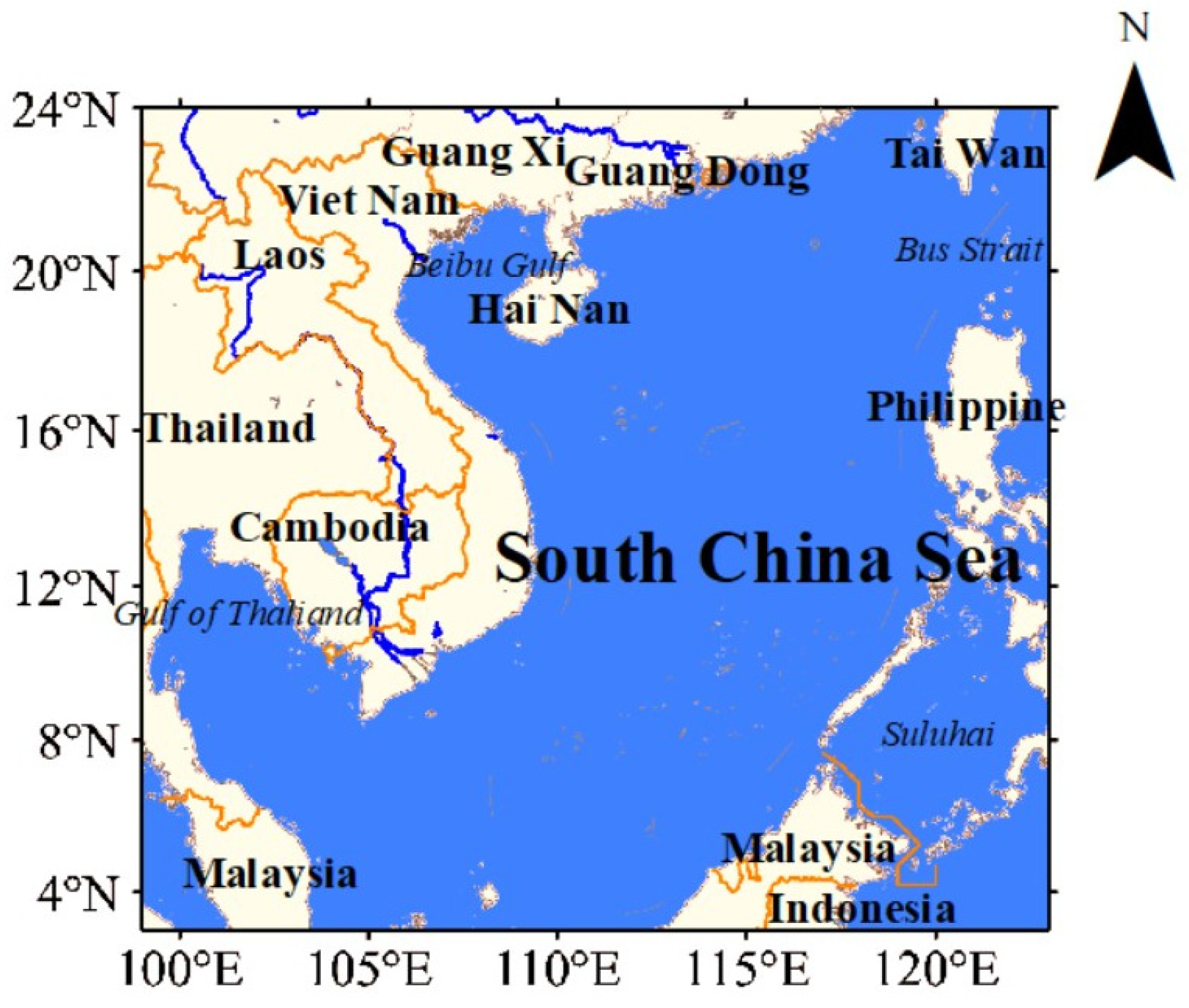
2.1. Data Sources

The zonal extent of the study area ranged from 3° N to 23° N, and the longitudinal extent was from 99° E to 123° E (Figure 1). To precisely identify El Niño and La Niña events, the Ocean Niño Index (ONI) of the National Oceanic and Atmospheric Administration (NOAA) was utilized, and an ONI map was generated (Figure 2). The ONI represents the three-month rolling average of the sea surface temperature (SST) in the Niño 3.4 region (5°N–5° S, 170°–120° W). In accordance with the Climate Prediction Center of NOAA, El Niño and La Niña events are classified when five consecutive ONI values exceed +0.5 °C (El Niño) or fall below −0.5 °C (La Niña), respectively. Additionally, for at least three overlapping three-month periods, events with ONI values within these thresholds are categorized as moderate, strong, or very strong El Niño events, following the same criteria as those for classifying weak, moderate, strong, and very strong El Niño events [20].

For the SST analysis, the ERA5 reanalysis monthly mean dataset covering the period from December 1958 to December 2024 was utilized at a spatial resolution of 0.25° × 0.25°. The ERA5 dataset was chosen for this study due to its high-resolution data on SST and meteorological elements, which are essential for analyzing small-scale ocean–atmosphere interactions in the South China Sea and understanding ENSO’s differential impacts on sea temperatures. Although the ERA5 data have certain limitations during the period from 1958 to 1980—such as less advanced data collection technology and sparse observation stations in some ocean areas, particularly marginal seas like the South China Sea, leading to uncertainties in SST data—it is important to note that the ERA5 data underwent rigorous quality control and assimilation processes. Therefore, they remain valuable for analyzing large-scale climate features and long-term trends. Detailed comparisons and rigorous validation with HadISST (Hadley Centre Sea Ice and Sea Surface Temperature dataset) show that the ERA5 data largely align with other datasets in reflecting ENSO-related SST anomaly trends, despite minor differences in some individual years or seasons. These discrepancies do not affect the overall usability and value of ERA5 data in this study. Additionally, the ERA5 monthly mean sea surface wind field data provide detailed spatiotemporal insights into atmospheric phenomena, with the same timing and resolution.

Since data for January and February 2025 were unavailable, the dataset includes summer data for 63 years and winter data for 62 years.

The seasons are defined as follows: spring (March–May), summer (June–August), autumn (September–November), and winter (December–February). This seasonal framework enables a detailed examination of the influences of El Niño and La Niña at different times of the year within the study area.

Based on ONI, seven strong El Niño events were identified during 1965–1966, 1972–1973, 1982–1983, 1986–1987, 1997–1998, 2009–2010, 2015–2016 and 2023–2024. The strong La Niña events of 1964–1965, 1970–1971, 1975–1976, 1988–1989, 1998–2001, 2007–2008, 2010–2012, and 2020–2021 were selected. This study examines the relationship between strong ENSO events and SST in the South China Sea, with particular attention paid to La Niña events.

In accordance with established practices [16,20], the year when the peak of a warm (El Niño) or cold (La Niña) event occurred was designated as “0 years”, and subsequent years were marked as “years + 1”, “years + 2”, and so on. Utilizing this framework, we calculated the mean SST for all identified strong El Niño years to represent the conditions during “El Niño years 0”. Similarly, the mean SST for a specified strong La Niña year can be employed as a baseline for “La Niña year 0” (

Table 1. Chronology of mean state of SST for El Niño and La Niña events (the red-marked parts of the table represent “Year − 1” to “Year + 1” of El Niño events, while the blue-marked parts represent “Year − 1” to “Year + 1” of La Niña events).

El −1	1965	1971	1981	1985	1996	2008	2014	2022
El 0	1966	1972	1982	1986	1997	2009	2015	2023
El +1	1967	1973	1983	1987	1998	2010	2016	2024
La −1	1963	1969	1974	1987	1994	1997	2006	2009	2019
La 0	1964	1970	1975	1988	1995	1998	2007	2010	2020
La +1	1965	1971	1976	1989	1996	1999	2008	2010	2021

). This method enables a direct comparison of SSTAs associated with these two ENSO phases, highlighting their impact on the South China Sea.

2.2. Methods

The anomalies of key meteorological elements, such as evaporation, cloud cover, heat flux, and precipitation, of El Niño and La Niña events from 1958 to 2024 were analyzed by employing ERA5 data. Additionally, the spatial distribution of shear kinetic energy over the South China Sea during ENSO events was also studied to explore the atmospheric bridge effect.

In order to evaluate the correlation between meteorological elements and SST more precisely, the passive weighting method was adopted. The range function was utilized to calculate the data range of each array. The data range represents the degree of difference between the maximum and minimum values in the array and can serve as an indicator of the weight. Subsequently, the data range of each array was divided by the sum of all the data ranges to obtain the weight of each array. To ensure the normalization of the weights, they were processed. Passive weighting is a technique commonly employed in data analysis, optimization, and decision-making. This method assigns weights in accordance with the intrinsic importance of different factors or data points, such that more significant elements have a greater impact in the analysis while reducing the weight of less influential elements. The term “passive” indicates that weights are derived from inherent data characteristics or predefined criteria, rather than through active operations. This approach enhances the reliability of our results.

Using this method, the correlation of meteorological anomalies, SSTAs, and shear kinetic energy (K) in summer and winter of El Niño and La Niña years, covering “−1” to “+1” years, was calculated. The specific mathematical calculation method is as follows:

$$S=(c\_et+c\_pt+c\_st+c\_ct+c\_tt)$$

(1)

$$\begin{gathered} weight\left(1\right)=c_{et}/\mathsf{\Sigma }S;weight\left(2\right) \\ =c\_pt/\mathsf{\Sigma }S;weight\left(3\right) \\ =c\_st/\mathsf{\Sigma }S;weight\left(4\right) \\ =c\_ct/\mathsf{\Sigma }S;weight\left(5\right) \\ =c\_tt/\mathsf{\Sigma }S; \end{gathered}$$

(2)

$$K={\displaystyle \frac{1}{2}}\ast \rho (u^2+v^2)$$

(3)

The definitions of Formulas (1) and (2) are presented as follows: c_et represents the correlation between the evaporation anomaly and the SSTA; c_pt represents the correlation between the precipitation anomaly and the SSTA; c_st represents the correlation between the net heat flux anomaly and the SSTA; c_ct represents the correlation between the cloud cover anomaly and the SSTA; c_tt indicates the correlation between the temperature anomaly and the SSTA; and S denotes the aggregate weight of the correlations between the SSTA and anomalies in evaporation, precipitation, net heat flux, cloud cover, and temperature. Specifically, weight(1) represents the weighting factor for the correlation between evaporation anomalies and SSTA; weight(2) represents the weighting factor for the correlation between precipitation anomalies and SSTA; weight(3) represents the weighting factor for the correlation between net heat flux anomalies and SSTA; weight(4) represents the weighting factor for the correlation between cloud cover anomalies and the SSTA; and weight(5) represents the weighting factor for the correlation between temperature anomalies and SSTAs.

Formula (1) was used to define the correlation coefficients involved in the calculation of weights, which were used to represent the degree of association between different meteorological element anomalies and SSTAs, rather than for regression analysis to obtain prediction results and probability values.

To achieve normalization of the weights, each weight value in the array was divided by the sum of all weight values within the array, ensuring that the total sum of the weights equaled 1. This normalization process ensured that the relative importance of each weight was comparable in the analysis and eliminated potential biases arising from differences in the absolute values of the weights during calculations.

In Formula (3), ρ represents the air density, and u and v denote the meridional and zonal wind speeds, respectively. K represents the shear kinetic energy.

3. Result

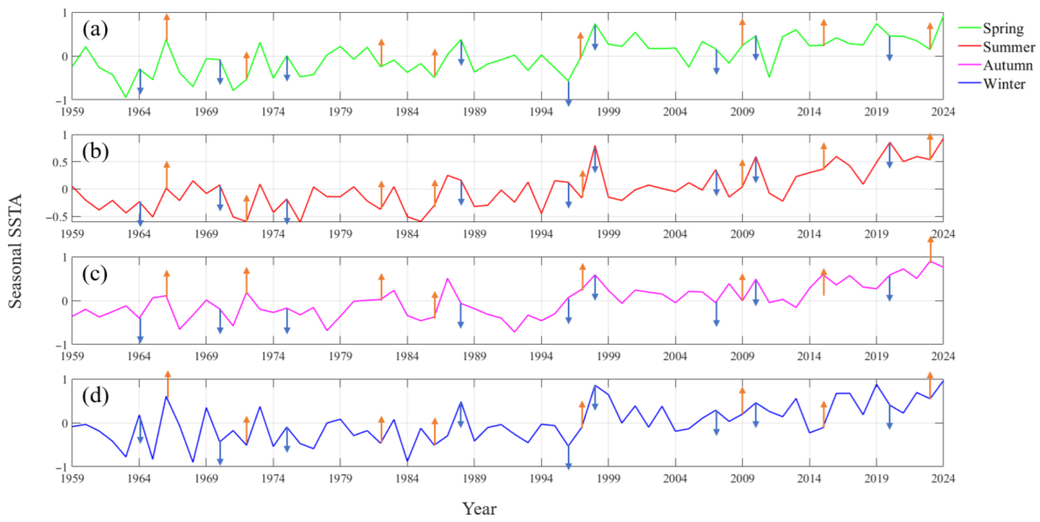
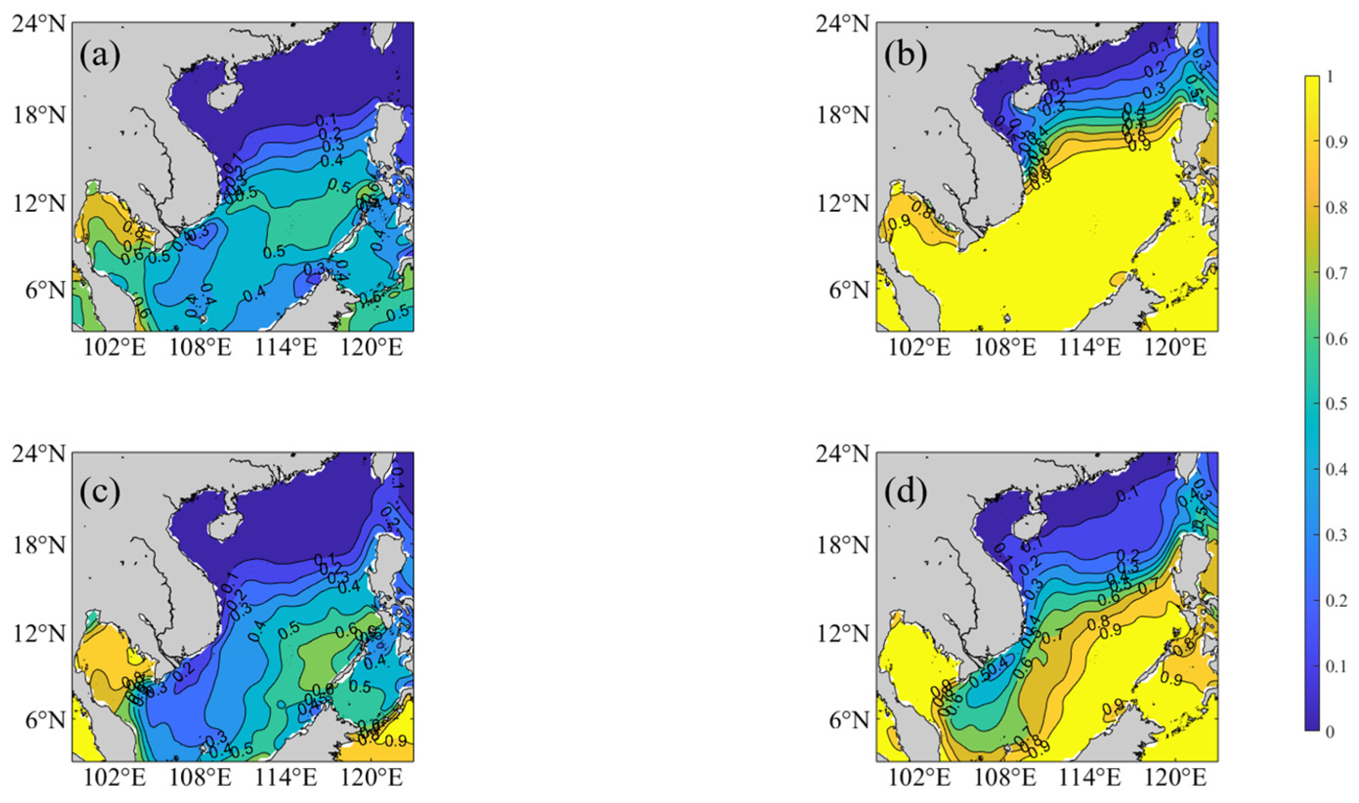
3.1. Seasonal Variation in SSTAs in South China Sea

The SST distribution in the South China Sea has an obvious spatial pattern, showing an obvious gradient from north to south. South of 17° N, the isotherms run along a northeastern–southwest direction, while north of 17° N, the isotherms run along an east–west direction. This results in a significant temperature difference between the North and South regions, especially in spring and winter when this contrast is most pronounced. In summer, the whole South China Sea SST increased significantly, and the temperature was between 28 and 30 °C (Figure 3). A notable exception, however, is the low-temperature region off the east coast of Vietnam, where the SST can drop to around 28 °C due to factors such as updrafts, the Vietnam Cold Vortex effect, and the cold filament phenomenon caused by the easterly jet stream near the sea [21].

In autumn, changes in local ocean circulation and heat flux lead to reduced SST and increased regional temperature differences, with the SST generally ranging between 25 °C and 28 °C. In addition, the SST front moves southward between 105° and 110° E, mainly due to strong advection of the monsoon-driven western boundary current off the coast of Vietnam. This phenomenon reduces atmospheric precipitation in warm pools 10° N south of the Indo-Pacific region.

In addition, changes in ENSO are strongly correlated with interannual fluctuations in the “cold tongue index”, which reflects the SST in a region with latitudes of 5°–10° N and longitudes of 106°–111° E. The index is an important tool for monitoring and predicting SST changes in the South China Sea and its related climate impacts [22,23].

The spring SST of El Niño years is positive in 1965 and 2009, and negative in the other years. Moreover, except for 1965, all years exhibit an upward trend in the annual average of El Niño “+1”. The La Niña years feature negative anomalies in 1971 and 1995, while the remaining years show positive anomalies. All La Niña “+1” years demonstrate a downward trend annually. In summer El Niño years, the SST presents negative anomalies in 1972, 1982, and 1986, and positive anomalies in other years. All years except 1965 show rising anomalies in the annual average of El Niño “+1”. Similarly, in La Niña years, the SST shows negative anomalies in 1964, 1971, and 1995, while it shows positive anomalies in other years. Except for 1971, the remaining years show a downward trend in La Niña “+1” annually. In autumn, all El Niño years except 2009 exhibit negative SSTAs. All years except 1965 show an upward trend in the annual average of El Niño “+1”. For La Niña events, the SST shows negative anomalies in 1964, 1971, and 1975, while it shows positive anomalies in the other years. All La Niña “+1” years show a downward trend every year. The winter SST of all El Niño years presents positive anomalies, except for 1986, and all other years except 1965 show an upward trend in El Niño “+1” years. In La Niña years, the SST shows positive anomalies in 1998, 2010, and 2020, and negative anomalies in the other years. The trend of change alternates in La Niña “+1” years.

It is important to note that, in addition to the SSTAs during El Niño and La Niña years, the seasonal SST in El Niño “+1” years and La Niña “+1” years exhibit distinct patterns of increase or decrease (Figure 4). To investigate the correlation between seasonal SSTAs and ENSO events, the following section will analyze SSTAs from El Niño “−1” to El Niño “+1” years and La Niña “−1” to La Niña “+1” years, examining their relationship with ENSO and the lead–lag dynamics. During these periods, changes in atmospheric circulation—such as variations in surface temperature, humidity, cloud cover, monsoon patterns, and wind fields—affect surface heat fluxes and ocean currents in the South China Sea. Depending on the different stages of SSTA evolution, these changes may result in warming or cooling effects [24]. Consequently, both summer and winter SST variations are influenced by solar radiation, dynamic processes, and atmospheric anomalies.

El Niño events typically have a definite duration, and the sea surface temperature in the South China Sea exhibits periodic variation characteristics related to ENSO events across different seasons. Figure 4 illustrates the relationship between the seasonal average sea surface temperature in the South China Sea and ENSO events from 1958 to 2021, revealing the periodic features associated with ENSO events in the time series.

As depicted in Figure 2, the events of El Niño and La Niña occur alternately, and the decline period of El Niño overlaps with the development period of La Niña. Consequently, the SST in the South China Sea in “0” and “+1” years of El Niño events exhibits opposite patterns. ENSO events are asymmetrical, and La Niña is typically less intense than El Niño. Additionally, the recession period of La Niña has the least overlap with the growth period of El Niño. Therefore, the SSTAs in the South China Sea in “0” and “+1” years of La Niña events do not follow the same rules as those in El Niño events. Through analyzing the SSTAs of El Niño events and La Niña events in “0” and “+1” years, it is discovered that there are disparities in the SSTA patterns of El Niño events in these two years, while the difference in the SST anomaly patterns of La Niña events is minor.

A periodic analysis reveals that the peak of positive SSTAs of El Niño events occurs in the winter of El Niño “0” years, and the peak of negative SSTAs of La Niña events occurs in the summer of La Niña “+1” years. In El Niño events, the positive SSTAs initially emerge in “−1 years” and are more pronounced in “0”~“+1” years. The negative anomaly appears in the “−1” year, but reverts to a positive anomaly later in the “0” year. In contrast, during the La Niña event, a positive anomaly is observed in years −1 to 0, followed by a negative anomaly in the second half of year 0. A stronger negative anomaly emerges in the “+1” year; compared with La Niña years, the winter SST increases more conspicuously in El Niño years, and there is a slight deviation between June and September in El Niño years. La Niña usually lasts from September to May (Figure 5).

The ONI was employed to examine the correlation between El Niño events and La Niña events and SSTAs in the South China Sea during 1958–2021. The correlation between El Niño events, La Niña events, and the ONI is presented in Figure 6. These data illustrate the relationship between the seasonal SST in the South China Sea from 1958 to 2021 and different phases of ENSO (El Niño events and La Niña events), with a time series offset of up to 11 months to account for potential lags or lead times. The results indicate that the correlation coefficient attains the maximum value of −0.59 nine months prior to the El Niño event and −0.67 two months prior to the La Niña event. These findings are in line with previous studies, such as that of Yukihiro Niu (1985), which discovered that the SST phenomenon in the Niño 3.4 region is often approximately 9 months earlier than the La Niña event [25], and the SST in remote ocean areas is closely related to the ENSO event. The peak of tropical Pacific SST occurred 2 to 6 months after the peak of the ENSO event [24,26]. In Figure 5, the peaks represent the maximum or minimum values of the SST in the South China Sea during different years (from ‘−1 year’ to ‘+1 year’) within the El Niño and La Niña events. These peak values are closely related to the development stage of the ENSO event. The reason for the peak of the tropical Pacific SST occurring 2–6 months after the peak of the ENSO event is the complex interaction between the ocean and atmosphere systems. After the ENSO event reaches its peak, processes such as heat transfer in the ocean and the adjustment of atmospheric circulation require a certain amount of time, resulting in a delay in the response of the tropical Pacific SST, which reaches its peak 2–6 months later (Figure 6). This pattern is similar to the seasonal frequencies of El Niño and La Niña events reported by Alizadeh (2022) [27]. In the subsequent step, we will discuss the correlation between seasonal SSTAs in the study area and the ONI, and investigate the rule of its lead and lag.

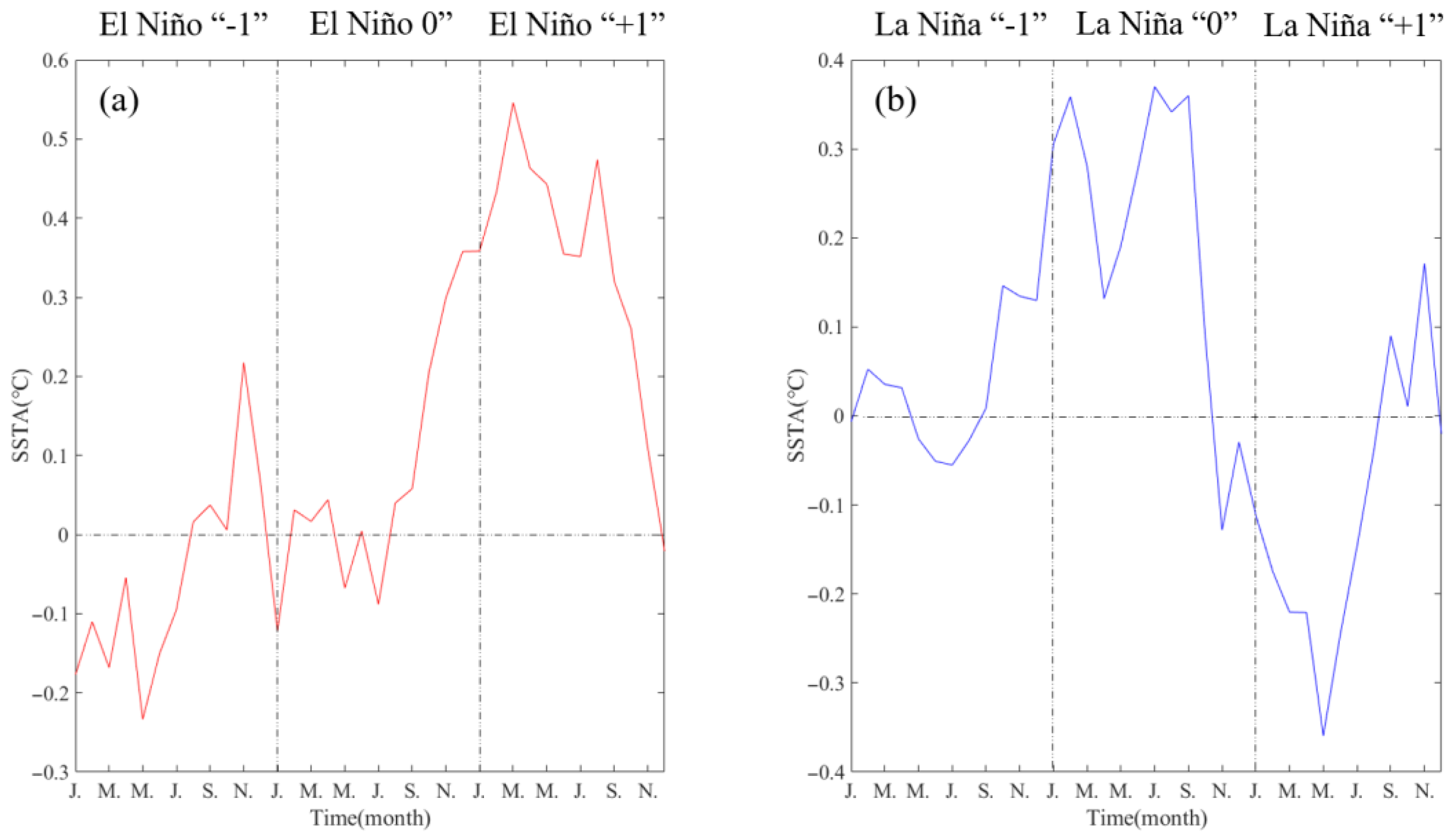
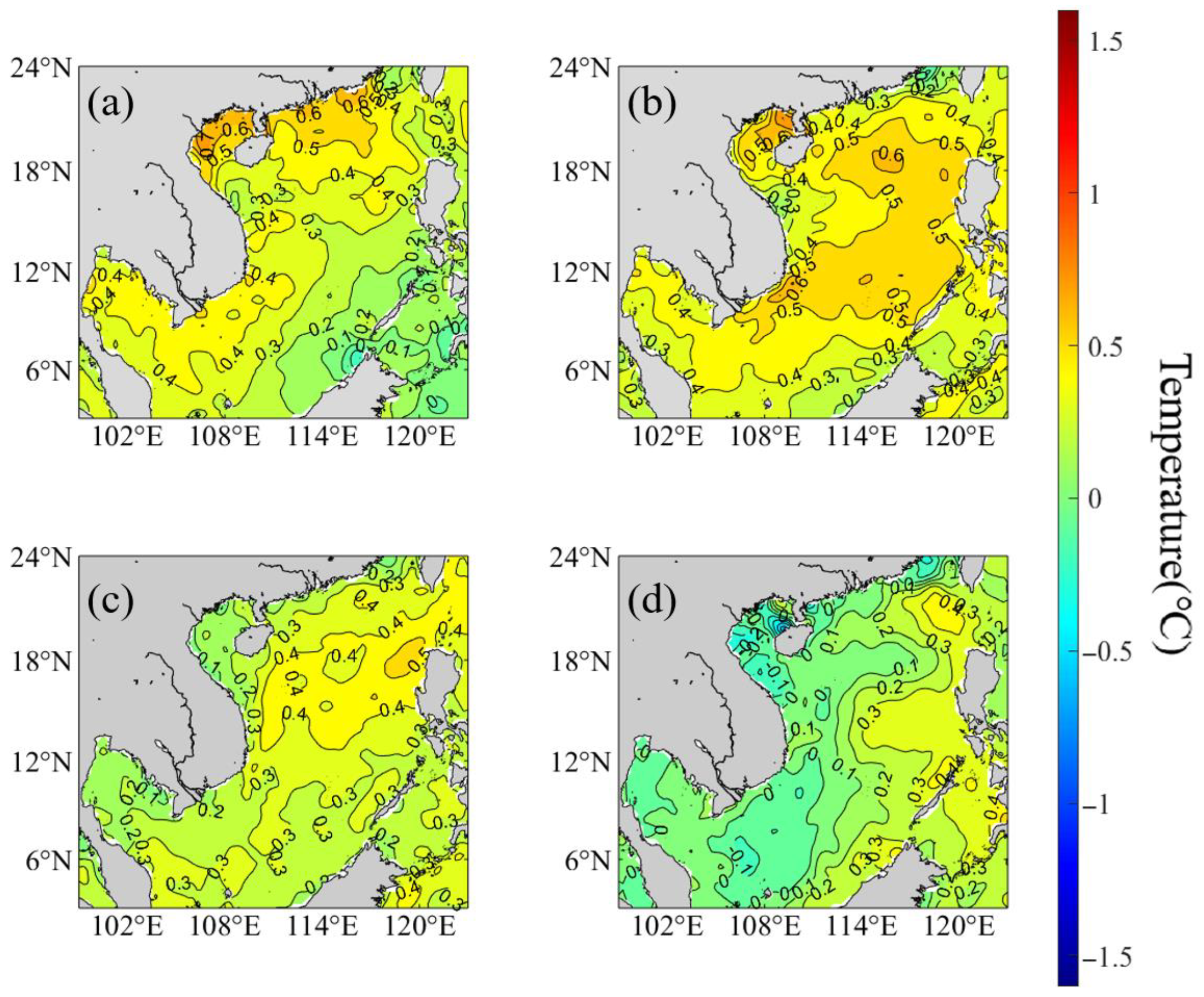
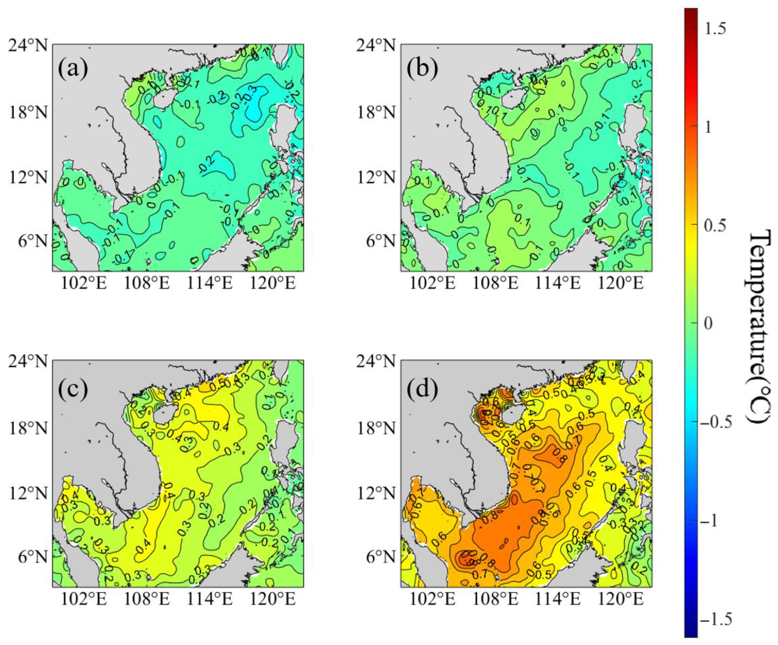
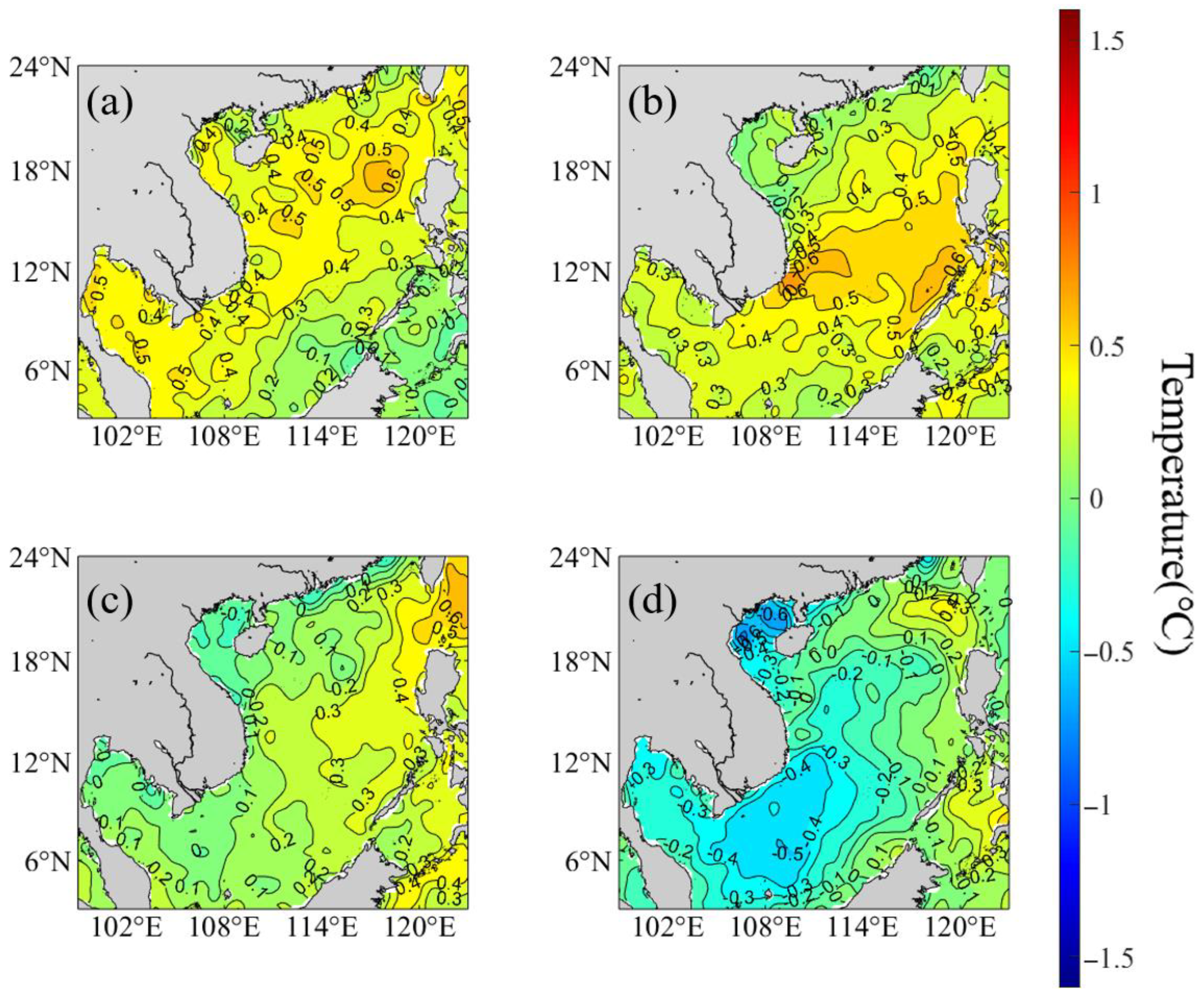
3.2. Analysis of SSTA Assemblages in South China Sea During Strong ENSO Events from 1958 to 2021

During El Niño events, SSTAs are more pronounced in both summer and winter. At the end of winter and prior to the beginning of spring, abnormal atmospheric circulation patterns induce changes in heat flux, resulting in positive SST shifts. Under the influence of geostrophic advection, the positive anomaly gradually weakens, turns into a negative anomaly, and reverts to a positive anomaly again in late summer and early autumn. It is noteworthy that SSTAs respond to El Niño events with a lag, typically occurring between “−1 year” and “+1 year” (Figure 7, Figure 8 and Figure 9).

During the La Niña event, the sea surface temperature continuously drops from “−1 year” to “+1 year”, presenting an evident negative trend. In spring, the anomaly transforms from a weak negative one to a more pronounced negative anomaly. In summer, there is no conspicuous anomaly at the beginning of the SST, but it turns negative at the end of the season. In autumn, no significant outliers are identified. In winter, the positive anomaly converts into a strong negative anomaly and gradually weakens at the end of the season (Figure 10, Figure 11 and Figure 12).

For El Niño “−1” year (Figure 13a), in spring (green line), the correlation coefficient between SSTAs and El Niño reaches a maximum value of 0.40 at a lag of 3 months, perhaps due to the delay in the interaction between the atmospheric circulation and the ocean affecting heat exchange. In summer (red line), the correlation coefficient is −0.68 at a lag of 9 months, possibly affected by factors such as the abnormal atmospheric circulation changing the ocean heat flux. In autumn (pink line), the correlation coefficient is −0.40 at a lag of 4 months, which is related to the ocean thermal inertia and other factors. In winter (blue line), the correlation coefficient is 0.24 at a lag of 0 months, indicating that the influence is manifested quickly in winter due to the atmospheric circulation and ocean conditions.

For La Niña “−1” year (Figure 13b), in spring (green line), the correlation coefficient is 0.28 at a lead of 6 months, and the previous changes have already affected the spring sea temperature in the South China Sea. In summer (red line), the correlation coefficient is 0.52 at a lag of 8 months, and the changes in the atmospheric circulation and ocean processes have a significant impact at this time. In autumn (pink line), the correlation coefficient is 0.15 at a lag of 1 month, and the response of the sea temperature to La Niña manifested at this lag time due to the air–sea interaction. In winter (blue line), the correlation coefficient is 0.22 at a lag of 0 months, and the influence is quickly reflected.

For El Niño “0” years (Figure 14a), in spring (green line), the correlation coefficient shows periodic changes without an obvious maximum value, which is affected by the intertwined influence of multiple complex factors. In summer (red line), the correlation coefficient is −0.47 at a lead of 9 months, and the previous changes in the atmospheric circulation and ocean environment have a significant impact. In autumn (pink line), the correlation coefficient is −0.26 at a lead of 3 months, which is related to the atmospheric circulation and ocean conditions in that season. In winter (blue line), the correlation coefficient is 0.33 at a lag of 9 months, and the influence is presented at a lag due to the atmospheric circulation and ocean processes.

For the La Niña “0” years (Figure 14b), in spring (green line), the correlation coefficient shows periodic changes without an obvious maximum value because of the dynamic changes in the ocean-atmosphere system. In summer (red line), the correlation coefficient is −0.45 at a lag of 15 months, and the influence of the atmospheric circulation and ocean processes takes a long time. In autumn (pink line), the correlation coefficient is 0.20 at a lag of 12 months, which is related to the air–sea interaction. In winter (blue line), the correlation coefficient is −0.16 at a lag of 15 months, and the influence is manifested at a long lag.

In the El Niño “+1” years (Figure 15a), in spring (green line), the correlation coefficient shows periodic changes without an obvious maximum value due to the comprehensive influence of multiple factors. In summer (red line), the correlation coefficient is 0.32 at a lead of 12 months, and the previous influence has persistence. In autumn (pink line), the correlation coefficient is 0.27 at a lead of 12 months, which is related to the previous long-term influence and the seasonal changes. In winter (blue line), the correlation coefficient is 0.20 at a lead of 9 months, and the influence of the previous atmospheric circulation and ocean processes is manifested at this time.

In the La Niña “+1” year (Figure 15b), in spring (green line), the correlation coefficient shows periodic changes without an obvious maximum value because the ocean–atmosphere system is in adjustment. In summer (red line), the correlation coefficient is −0.55 at a lag of 9 months, and the influence of the atmospheric circulation and ocean processes is significant. In autumn (pink line), the correlation coefficient is −0.38 at a lag of 4 months, which is related to the air–sea interaction. In winter (blue line), the correlation coefficient is −0.16 at a lead of 3 months, and the previous influence is manifested at this time.

In summary, during El Niño events, the strongest correlations between SSTAs and the ONI were observed in summer and winter, while during La Niña events, the strongest correlations occurred in summer and autumn. Despite the generally stronger correlation in summer for both El Niño and La Niña events, the maximum lag or lead times varied across different years, with overlap in the lead–lag times between El Niño “−1” to El Niño “+1” and La Niña “−1” to La Niña “+1”. This overlap may be attributed to the use of averaged global SSTA values in the calculations. To further validate these conclusions, we plan to conduct a two-dimensional correlation analysis between the ONI and seasonal SSTAs to ensure the robustness of our findings.

The correlation between SSTAs and the ONI in the four seasons of El Niño and La Niña events is verified in a two-dimensional manner. In the case of El Niño events, the lead time of spring is 9 months, the lead time of summer is 3 months, the lead time of autumn is 8 months, and the lead time of winter is 1 month. The verification results demonstrate that there is a strong correlation between 2D SSTAs and ONIs corresponding to lead and lag events. Among them, both summer and winter exhibit a strong correlation in the southern part of the study area, and in autumn, a relatively strong correlation is shown in the southwest and southeast parts of the study area. (Figure 16). In the case of La Niña events, verification was conducted for 6 months ahead in spring, 8 months behind in summer, 12 months ahead in autumn, and 9 months behind in winter. The verification results indicated that there was a strong correlation between 2D SSTAs and ONIs corresponding lead and lag events. Both spring and summer displayed a strong correlation in the southern part of the study area. Winter showed a strong correlation in the southwest and southeast of the study area, while autumn presented a weak correlation, which was consistent with our previous conclusions (Figure 17).

Through verification, in El Niño and La Niña events, SSTAs and ONIs show a strong correlation in both summer and winter. In El Niño events, there is a strong correlation three months ahead in summer and a strong correlation one month behind in winter. In La Niña events, the summer lag of 8 months shows a strong correlation, and the winter lag of 9 months shows a strong correlation. This difference in seasonal correlation might be attributed to a slight deviation in the timing of El Niño events between June and September, while most La Niña events occur between October and February [28]. We can also find that the correlation of the four seasons in the southern part of the study area is stronger than that in the northern part. Then, what are the factors contributing to the response of the South China Sea to the events of El Niño and La Niña?

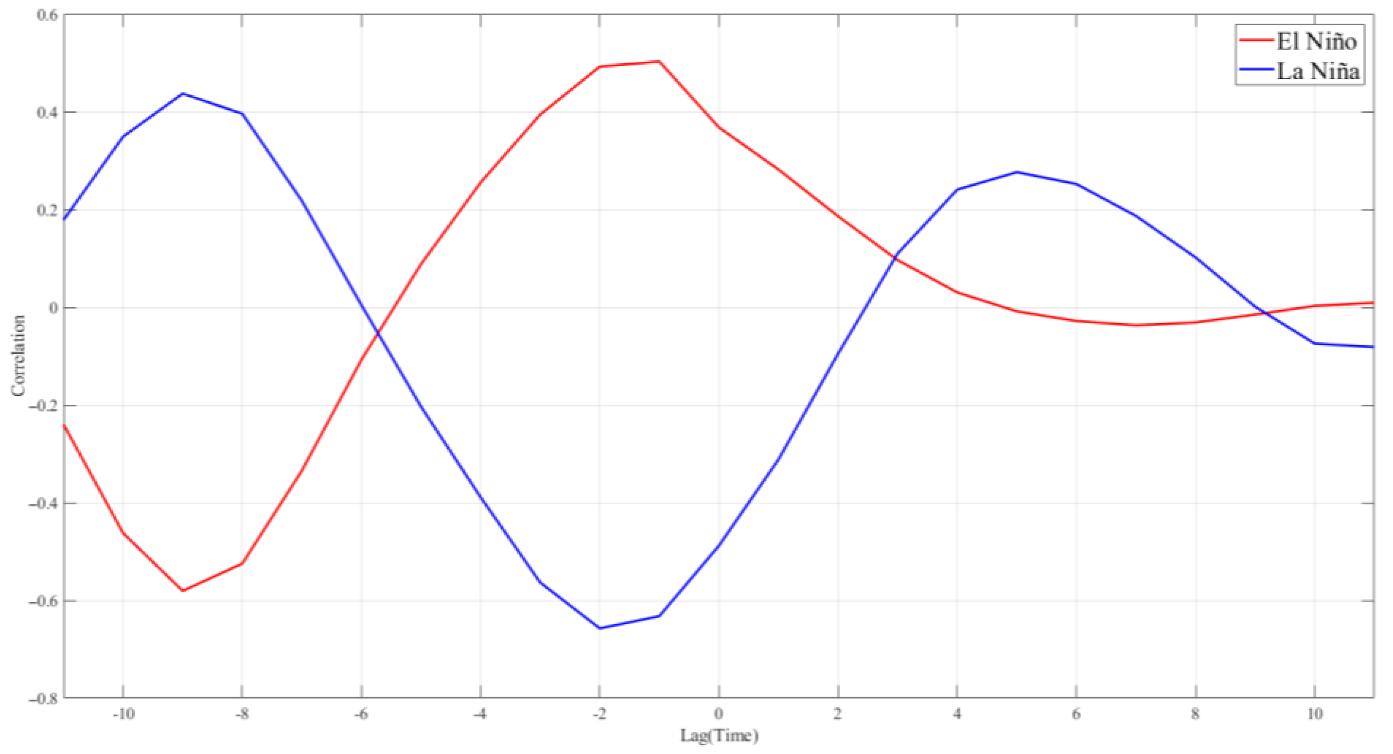
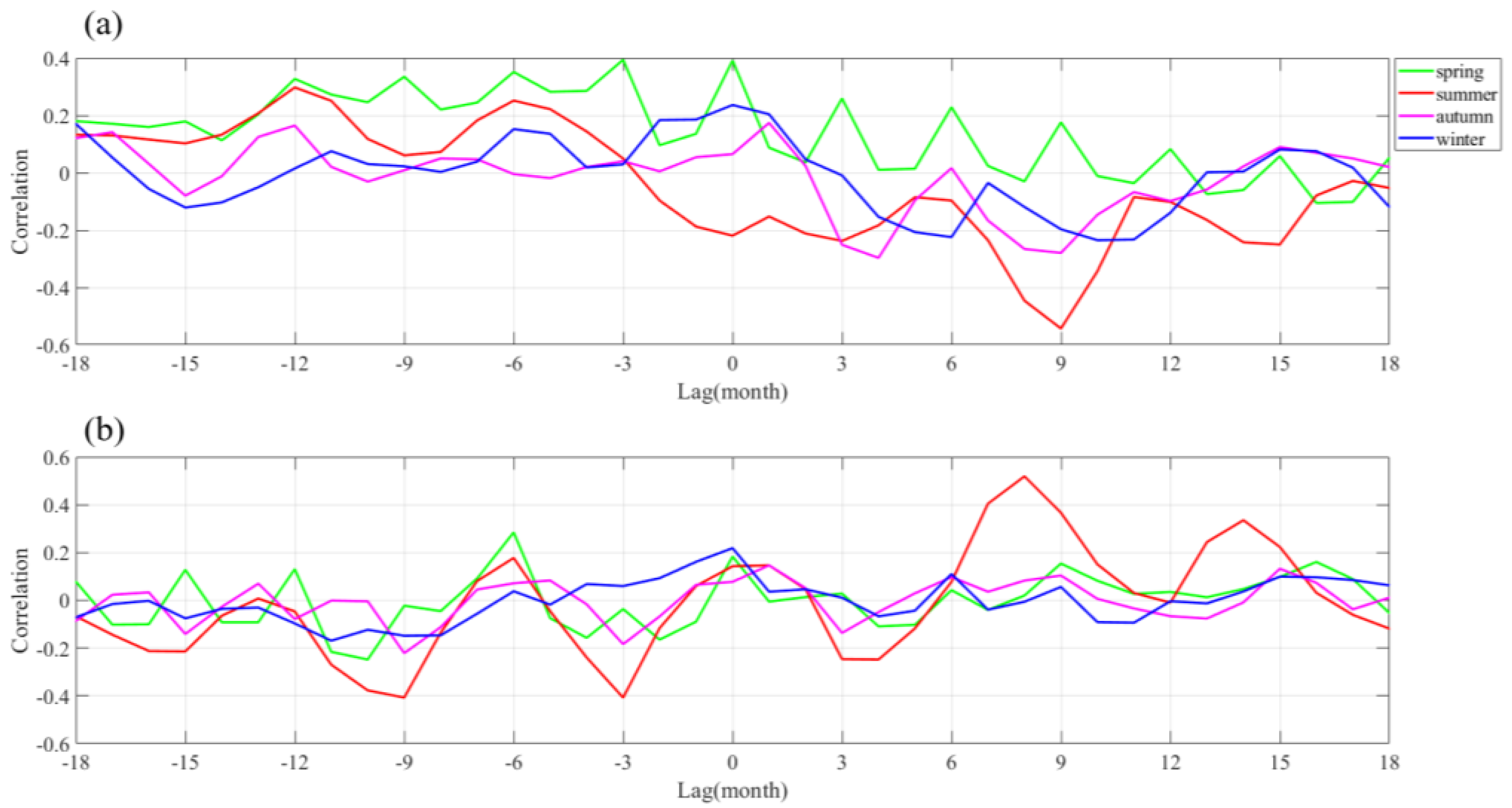
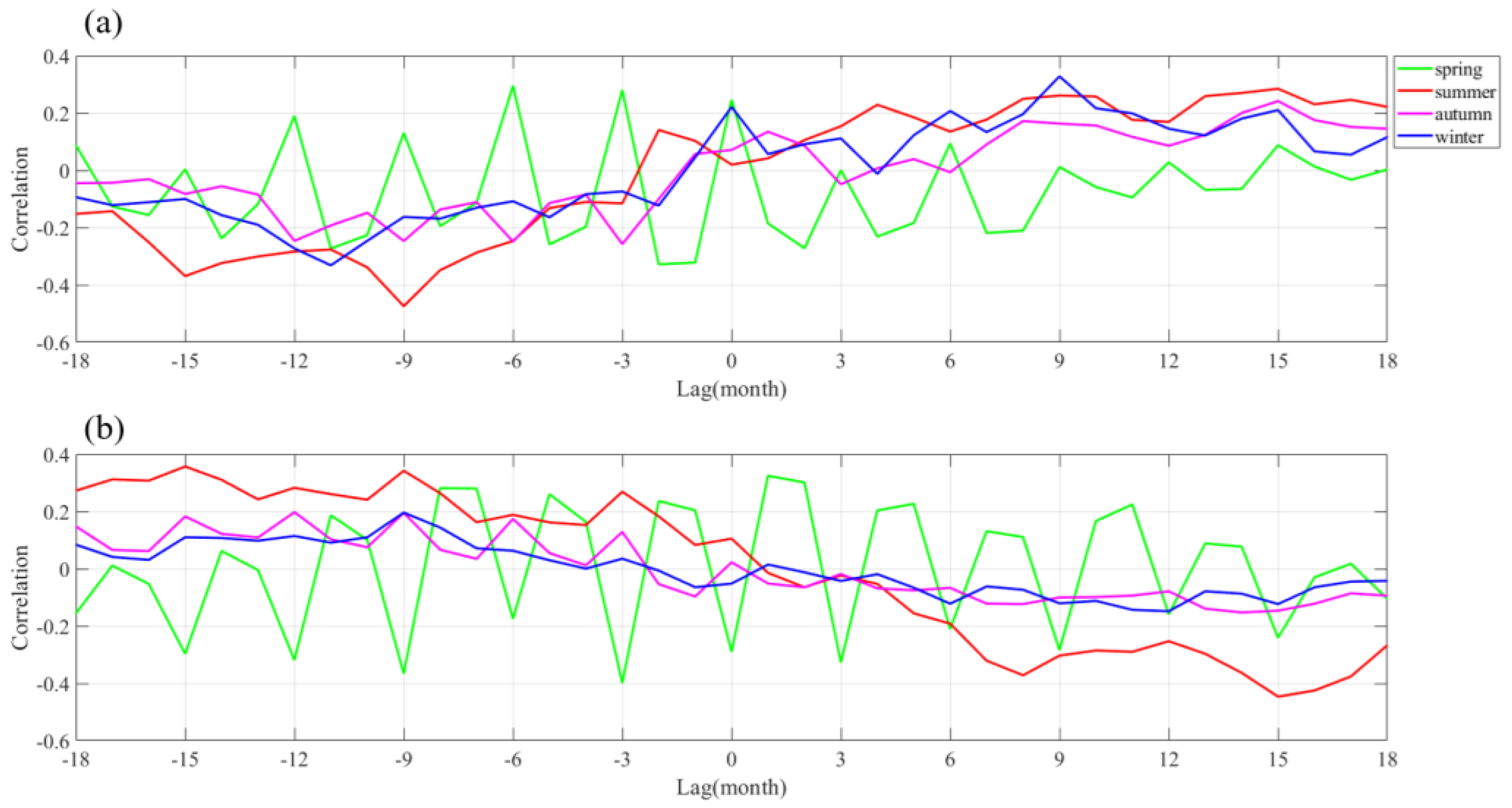
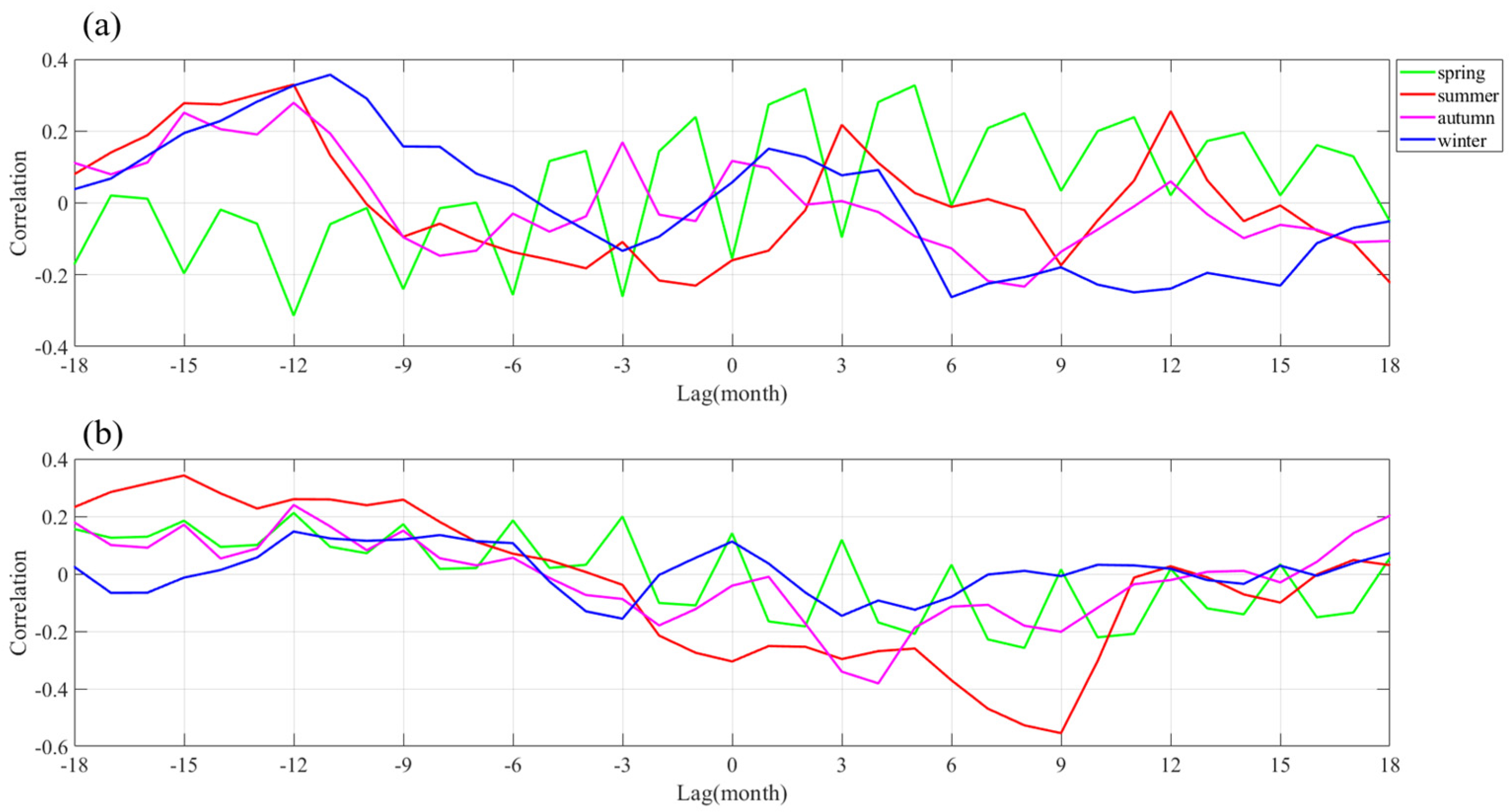
3.3. Correlation Analysis of Relevant Elements

Dai Nianjun et al. [29] emphasized that the inter-annual variation in the South China Sea summer monsoon is closely linked to ENSO events. Furthermore, SST has a direct impact on meteorological factors such as evaporation, net heat flux, cloud cover, and precipitation [30]. Research indicates that during El Niño and La Niña events, the regional precipitation anomalies in the Niño 3.4 region exhibit distinct patterns: During El Niño events, positive anomalies peak around the New Year, while negative anomalies peak in early autumn [1]. Additionally, both ENSO and the East Atlantic pattern are significantly correlated with precipitation variability in Southwest Asia [31]. The relationship between oceanic and continental precipitation anomalies is particularly strong in the tropical Pacific, where ENSO influences are evident [28]. The evolution of ENSO also significantly affects the precipitation of the Indian summer monsoon [32]. Its impact on winter precipitation in South China is asymmetrical, with a positive correlation in El Niño winters and a negative correlation in La Niña winters [33]. Notably, the response of winter precipitation to El Niño events is more pronounced in southeastern China [34].

To further explore the relationship between regional SSTAs and ENSO events, we conducted a comprehensive analysis by calculating the correlation between SSTAs and precipitation anomalies, evaporation anomalies, cloud cover anomalies, and net heat flux anomalies. This multifaceted approach aims to elucidate the interactions between these meteorological factors and how they are influenced by ENSO, thereby deepening our understanding of their interconnections and potential impacts on regional weather patterns.

The weighted results obtained from Formulas (1) and (2) show that precipitation anomalies and net heat flux anomalies have strong correlation weights with SST. By comparing the heat flux and precipitation anomalies in the four seasons of El Niño and La Niña from 1958 to 2021, it is evident that the anomalies are more pronounced in winter and summer. Therefore, we calculated the correlation between various meteorological elements during El Niño (“−1 year” to “+1 year”) and La Niña (“−1 year” to “+1 year”), particularly in winter and summer. The calculation results are presented in

Table 2. Correlation between each meteorological element during El Niño (“−1 year” to “+1 year”) and La Niña (“−1 year” to “+1 year”).

Summer	Cloud	Evaproation	Net Heat Flux	Precipitation
El −1	0.36	−0.06	0.11	0.22
El 0	0.37	0.04	0.16	0.18
El 1	0.05	0.03	0.05	−0.02
Winter	Cloud	Evaproation	Net Heat Flux	Precipitation
El −1	−0.02	−0.03	−0.01	−0.04
El 0	0.08	−0.16	0.05	0.09
El 1	0.25	−0.31	−0.06	0.36
Summer	Cloud	Evaproation	Net Heat Flux	Precipitation
La −1	−0.02	−0.1	−0.06	0.05
La 0	0.04	0.06	−0.07	−0.09
La +1	0.16	−0.13	0.14	0.12
Winter	Cloud	Evaproation	Net Heat Flux	Precipitation
La −1	−0.02	0.06	−0.01	−0.02
La 0	0.47	−0.36	0.36	0.37
La +1	−0.20	0.18	−0.14	0

.

It is evident that in El Niño years, the relationship between meteorological variable anomalies and SST is most pronounced in summer, while in La Niña years, this relationship is more intense in winter.

Formula (3) was used to calculate the shear kinetic energy and analyze its correlation, with a threshold value of 0.5. When the absolute value exceeds 0.5, the correlation is considered significant, and a value close to 1 or −1 indicates a strong correlation.

There is no significant correlation between summer shear kinetic energy anomalies and SST in El Niño “−1” years. However, a strong negative association is evident in the southern region during the winter months. In El Niño “0” years, there is a significant positive correlation between shear kinetic energy and SST in the east region in summer. Conversely, winter shows a strong positive correlation in the central region and a significant negative correlation in the southwest region, exhibiting a bimodal pattern. During El Niño “1” years, there is a significant negative correlation in northwest China in summer, and a strong correlation in southwest, northeast, and southeast China in winter, presenting a tri-modal structure (Figure 18).

During the La Niña “−1” years, a positive correlative relationship can be witnessed between the anomalies of summer shear kinetic energy and sea surface temperatures within the central area. Throughout the winter months, such a correlative connection becomes more conspicuously manifested in the southwest region. In the La Niña “0” years, a notably strong positive correlation surfaces in the northwest region during the summer season. Come wintertime, negative correlations come to the fore in the southwest, northeast, and southeast regions, respectively, thus forging a trimodal configuration. In regard to the La Niña “1” years, a remarkably significant positive correlation springs up in the summer. Once winter sets in, a relatively robust positive correlation makes its appearance in the southwest region, while a comparatively powerful negative correlation reveals itself in the northwest region, once again giving rise to an inverse bimodal architecture (Figure 19).

The observed pattern of shear kinetic energy anomalies is significantly influenced by the interaction between meteorological elements and SST. The relationship is complex and multifaceted:

• Clouds: Clouds cause friction and reduce wind speed, which, in turn, affects the generation and distribution of shear kinetic energy by limiting vertical mixing of the atmosphere and altering boundary layer dynamics.
• Atmospheric Heating through surface heat flow enhances upward air movement, reduces air density, and accelerates air. An increase in airflow velocity results in an increase in shear energy by amplifying wind shear between atmospheric layers [35].
• Evaporation: Evaporation cools the ocean surface, increases air density, and reduces wind speed in the lower atmosphere. However, this process also increases moisture in the air, potentially enhancing convection and altering wind patterns, which can affect shear energy.
• Precipitation: Precipitation has a dual effect on shear energy. On one hand, it provides resistance to atmospheric flow and reduces wind speed. On the other hand, it is associated with strong convective systems, which can increase wind shear under certain conditions, depending on the specific dynamics of the precipitation event.

The interaction between these meteorological factors leads to changes in shear energy, especially in response to changes in sea temperature. Notably, shear energy anomalies are strongly correlated with SST, particularly in the summer for El Niño and the winter for La Niña. These relationships underscore the crucial role of ENSO-driven SST in shaping atmospheric circulation patterns, which, in turn, influence wind speed and shear kinetic energy in the region.

ENSO events also have a profound impact on SST in the South China Sea. During El Niño years, abnormal deep-sea temperatures in the central and eastern Pacific weaken the subtropical high in the Eastern Pacific. This alters the strength and direction of the southeast trade winds, affecting ocean currents and creating a feedback loop that amplifies SST. These changes in SST influence atmospheric circulation, convection, and precipitation patterns across the region [20].

Seasonal changes in sea temperature are another key factor. The influence of El Niño is most pronounced in summer, while that of La Niña is more significant in winter. Additionally, the topography of the region plays a crucial role in regulating these SSTs, and certain areas of the South China Sea are more susceptible to changes in ocean temperature due to local geographical features.

In summary, the relationship between shear kinetic energy, meteorological elements (such as cloud cover, heat flux, evaporation, and precipitation), and SST is essential for understanding seasonal and interannual variability in the South China Sea and its broader atmospheric and oceanic dynamics.

4. Conclusions

Using ERA5 data, the SST reanalysis, evaporation, cloud cover, net heat flux, precipitation, and 850 hPa wind field over the South China Sea during 1958–2021 were comprehensively analyzed. The results show a significant seasonal correlation and time lag between SST and ENSO.

The SST of the South China Sea in spring, summer, autumn, and winter of El Niño years is positive, whereas it is negative in La Niña years. Notably, during the “+1 year” following an El Niño event, the SST reverses from the initial “0 year” state. However, this clear opposite trend was not observed during the La Niña years. The correlation between SST in the South China Sea and the El Niño index in El Niño years is stronger than that in La Niña years.

There is a strong lag correlation between the SST in the South China Sea and the evolution of ENSO events in the tropical Pacific. Temporally, the correlation between El Niño events and a 9-month lead reaches its peak, while the correlation between La Niña events and a 2-month lead is the strongest. Seasonally, in El Niño events, there is a strong correlation between a 3-month lead in summer and a 1-month lag in winter. In La Niña events, the summer lag of 8 months shows a strong correlation, and the winter lag of 9 months shows a strong correlation.

Driven by changes in evaporation and cloud cover caused by ENSO, the abnormal atmospheric circulation significantly alters the net heat flux of distant ocean areas, leading to abnormal changes in SST. This effect is more pronounced in the summer of El Niño years than in the winter, possibly due to the increased influence of solar radiation on net heat flux and precipitation in summer. Additionally, in the seasons of El Niño and La Niña years, shear kinetic energy has a significant influence on SST, and its influence varies over time.

Enhancing our understanding of SSTAs in ENSO-affected areas is crucial for comprehending ENSO’s broader impact on the South China Sea. This knowledge is essential for improving climate change predictions and predicting the response of marine ecosystems in the region, and is vital for advancing both research and conservation efforts. However, several questions remain unresolved, particularly regarding potential changes in the spatial structure of ENSO in recent decades, which require further study [20]. In recent years, the Pacific Ocean SST has been categorized into EP (Eastern Pacific) and CP (Central Pacific) models [36]. Future studies can further explore the effects of these two models on SST in the South China Sea and their correlation. Additionally, the effect of ENSO on SST in the South China Sea appears to be influenced by topographic factors [14], which need to be further confirmed in subsequent studies. The contribution of shear kinetic energy to SST changes at different time scales is also worthy of further discussion. Moreover, global warming plays a significant role in regulating inter-watershed relationships, and studying ENSO’s response to global warming is an intriguing area for future research.

References

- Frequency of Different Types of El Niño Events Under Global Warming—Alizadeh—2022—International Journal of Climatology—Wiley Online Library. Available online: https://rmets.onlinelibrary.wiley.com/doi/10.1002/joc.7858 (accessed on 10 December 2024).
- Enochs, I.C.; Glynn, P.W.; Manzello, D.P. (Eds.) Coral Reefs of the Eastern Tropical Pacific: Persistence and Loss in a Dynamic Environment, 1st ed.; Coral Reefs of the, World; Springer: Dordrecht, The Netherlands; Imprint: Dordrecht, The Netherlands, 2017; ISBN 978-94-017-7499-4. [Google Scholar]
- Alizadeh, O. A Review of ENSO Teleconnections at Present and under Future Global Warming. WIREs Clim. Change 2024, 15, e861. [Google Scholar] [CrossRef]
- On the Decadal Changes of the Interannual Relationship Between ENSO and Tropical South Atlantic SST in Boreal Summer—Yang—2023—Geophysical Research Letters—Wiley Online Library. Available online: https://agupubs.onlinelibrary.wiley.com/doi/10.1029/2023GL104355 (accessed on 10 December 2024).
- Asymmetric Relationship between ENSO and the Tropical Indian Ocean Summer SST Anomalies in: Journal of Climate Volume 34 Issue 14 (2021). Available online: https://journals.ametsoc.org/view/journals/clim/34/14/JCLI-D-20-0546.1.xml (accessed on 10 December 2024).
- Yan, X.; Ren, J.; Ju, J.; Yang, S. Influence of Springtime Atlantic SST on ENSO: Role of the Madden–Julian Oscillation. Meteorol. J. 2018, 32, 380–393. [Google Scholar] [CrossRef]
- Lanzante, J.R. Lag Relationships Involving Tropical Sea Surface Temperatures. J. Clim. 1902, 9, 2568–2578. [Google Scholar] [CrossRef]
- Fei, Y.; Yi, X. Study of Long-Term Variational Trend of Sea Surface Temperature in the East China Sea. Adv. Mar. Sci. 2003, 21, 477–481. [Google Scholar] [CrossRef]
- Li, C.; Mu, M. El Niño Occurrence and Sub-Struface Ocean Temperature Anomalies in the Pacific Warm Pool. Chin. J. Atmos. Sci.-Chin. Ed. 2011, 23, 513–521. [Google Scholar] [CrossRef]
- Chao, Q.C.; Chao, J.P. Climatic Trends and Extremes of Tropical Cyclone Precipitation Affecting China and Its Key Economic Zones. Chin. J. Atmos. Sci. 2014, 38, 1029–1040. [Google Scholar] [CrossRef]
- Lin, T. Interdecadal variability of the relationship between ENSO and SST over the South China Sea. J. Mar. Meteorol. 2019, 39, 68–75. [Google Scholar] [CrossRef]
- Wu, G.X.; Meng, W. Gearing between the Indo-monsoon Circulation and the Pacific-Walker Circulation and the ENSO. Part I:_Data Analyses. CJAS 2011, 22, 470–480. [Google Scholar] [CrossRef]
- A Review of the El Niño-Southern Oscillation in Future—ScienceDirect. Available online: https://www.sciencedirect.com/science/article/abs/pii/S0012825222003300?via%3Dihub (accessed on 10 December 2024).
- Atlantic Warming Enhances the Influence of Atlantic Niño on ENSO—Wang—2024—Geophysical Research Letters—Wiley Online Library. Available online: https://agupubs.onlinelibrary.wiley.com/doi/10.1029/2023GL108013 (accessed on 10 December 2024).
- Hong, C.; Cho, K.-D.; Kim, H.-J. The Relationship between ENSO Events and Sea Surface Temperature in the East (Japan) Sea. Prog. Oceanogr. 2001, 49, 21–40. [Google Scholar] [CrossRef]
- Yu, S.; Zhou, F.; Fu, G.; Wang, D. Basic Characteristics of Low Frequency Oscillation of Surface Water Temperature in the South China Sea. Ocean Lakes 1994, 5. Available online: https://www.cnki.com.cn/Article/CJFDTotal-HYFZ199405012.htm (accessed on 11 December 2024).
- Diverse Impacts of ENSO on the Intensity of Tropical Western North Pacific Synoptic-Scale Disturbances During Boreal Summer—Gu—2023—Journal of Geophysical Research: Atmospheres—Wiley Online Library. Available online: https://agupubs.onlinelibrary.wiley.com/doi/10.1029/2023JD039238 (accessed on 10 December 2024).
- Yang, J.; Zhao, Y.; Wei, H.; Liu, S.; Zhang, G.; Long, H.; Li, S.; Xu, J. Holocene Sea Surface Temperature and Salinity Variations in the Central South China Sea. Mar. Micropaleontol. 2023, 181, 102229. [Google Scholar] [CrossRef]
- Expansion of Winter ENSO-Associated Rainfall Affected Area in Southeast Asia under Warmer Climate—Leong—2024—International Journal of Climatology—Wiley Online Library. Available online: https://rmets.onlinelibrary.wiley.com/doi/10.1002/joc.8358 (accessed on 10 December 2024).
- Diaz, H.F.; Kiladis, G.N. Atmospheric Teleconnections Associated with the Extreme Phase of the Southern Oscillation. In El Nino Historical & Paleoclimatic Aspects of the Southern Oscillation; Cambridge University Press: Cambridge, UK, 1992. [Google Scholar]
- The Teleconnection of El Niño Southern Oscillation to the Stratosphere—Domeisen—2019—Reviews of Geophysics—Wiley Online Library. Available online: https://agupubs.onlinelibrary.wiley.com/doi/10.1029/2018RG000596 (accessed on 10 December 2024).
- Wu, C.R.; Chang, C.W.J. Interannual Variability of the South China Sea in a Data Assimilation Model. Geophys. Res. Lett. 2005, 321. [Google Scholar] [CrossRef]
- Wang, C.; Wang, W.; Wang, D.; Wang, Q. Interannual Variability of the South China Sea Associated with El Niño. J. Geophys. Res. Atmos. 2006, 111. [Google Scholar] [CrossRef]
- Klein, S.A.; Soden, B.J.; Lau, N.C. Remote Sea Surface Temperature Variations during ENSO: Evidence for a Tropical Atmospheric Bridge. J. Clim. 1999, 12, 917–932. [Google Scholar] [CrossRef]
- Liu, Y.; Deng, Y. Sea Surface Temperature, Land Surface Temperature and the Summer Rainfall Anomalies over Eastern China. Clim. Environ. Res. 2002, 35, 10–14. [Google Scholar] [CrossRef]
- Zhang, P.; Xu, F. Spatial and Temporal Characteristics of the SSTA in the South China Sea from 1979 to 2017 and Its Correlation with the Walker Circulationn Anomaly. J. Mar. Meteorol. 2019, 39, 15–25. [Google Scholar] [CrossRef]
- Alizadeh, O. Amplitude, Duration, Variability, and Seasonal Frequency Analysis of the El Niño-Southern Oscillation. Clim. Change 2022, 174, 20. [Google Scholar] [CrossRef]
- Alizadeh-Choobari, O. Contrasting Global Teleconnection Features of the Eastern Pacific and Central Pacific El Niño Events. Dyn. Atmos. Oceans 2017, 80, 139–154. [Google Scholar] [CrossRef]
- Lian, T.; Wang, J.; Chen, D.; Liu, T.; Wang, D. A Strong 2023/24 El Niño Is Staged by Tropical Pacific Ocean Heat Content Buildup. Ocean-Land-Atmos. Res. 2023, 2, 11. [Google Scholar] [CrossRef]
- Wen, C.; Graf, H.F. The Interannual Variability of East Asian Winter Monsoon and Its Relation to the Summer Monsoon. Adv. Atmos. Sci. 2000, 17, 48–60. [Google Scholar] [CrossRef]
- Alizadeh-Choobari, O.; Adibi, P. Impacts of Large-Scale Teleconnections on Climate Variability over Southwest Asia. Dyn. Atmos. Oceans 2019, 86, 41–51. [Google Scholar] [CrossRef]
- Yang, X.; Huang, P. Restored Relationship between ENSO and Indian Summer Monsoon Rainfall around 1999/2000. Innovation 2021, 2, 100102. [Google Scholar] [CrossRef] [PubMed]
- Zhi, R.; Zheng, Z.; Feng, Q.G. Causes of Positive Precipitation Anomalies in South China during La Niña Winters. Clim. Dyn. Obs. Theor. Comput. Res. Clim. Syst. 2023, 61, 3343–3352. [Google Scholar] [CrossRef]
- Interpreting the Nonstationary Relationship Between El Niño–Southern Oscillation and the Winter Precipitation over Southeast China—Tang—2022—International Journal of Climatology—Wiley Online Library. Available online: https://rmets.onlinelibrary.wiley.com/doi/10.1002/joc.7570 (accessed on 10 December 2024).
- Niu, Z. Long-Period Variation of Surface Water Temperature in the South China Sea and Its Coupling with El Niño, Ocean University of China. Acta Oceanol. Sin. 1994, 16, 43–49. [Google Scholar]
- Li, J.; Huang, D.; Li, F.; Wen, Z. Circulation Characteristics of EP and CP ENSO and Their Impacts on Precipitation in South China. J. Atmos. Sol.-Terr. Phys. 2018, 179, 405–415. [Google Scholar] [CrossRef]