Enhancing Physical Spatial Resolution of Synthetic Aperture Sonar Images Based on Convolutional Neural Network

Abstract

The sonar image has limitations on the physical spatial resolution due to system configuration and underwater environment, which often leads to challenges for underwater targets detection. Here, the deep learning method is applied to enhance the physical spatial resolution of underwater sonar images. Specifically, the U-shaped end-to-end neural network which contains down-sampling and up-sampling parts is proposed to improve the physical spatial resolution limited by the array aperture. The single target and multiple cases are considered separately. In both cases, the normalized loss on the testing sets declines rapidly, and the predicted high-resolution images own great agreement with the ground truth eventually. Further improvements in resolution are focused on, that is, compressing the predicted high-resolution image to its physical spatial resolution limitation. The results show that the trained end-to-end neural network could map high resolution targets to the impulse responses at the same location and amplitude with an uncertain target number. The proposed convolutional neural network approach could give a practical alternative to improve the physical spatial resolution of underwater sonar images.

1. Introduction

Compared with electromagnetic waves, acoustic signals have the advantages of little attenuation, long propagation distance, and high fidelity, which has been the major transmission medium for underwater detection. Within, synthetic aperture sonar (SAS) is a worldwide underwater imaging method, that has the advantage of high performance and wide applicability [1,2,3,4,5]. Hence, SAS is applied in various fields, i.e., seafloor mapping, and underwater target detection. Although, the SAS achieves better performance than the conventional sonar method such as multibeam echo sounder (MBES) or side-scan sonar [6,7]. There are challenges that cannot be ignored, such as the complex and changeable underwater channel, the multipath effect, and the low robustness of sonar system calibration and post-processing algorithms, resulting in low resolution of sonar images [8,9,10,11,12,13]. These characteristics bring great challenges to the subsequent sonar image analysis and recognition.

Nowadays, as a powerful tool in image processing, deep learning methods are widely studied for the improvement of sonar imaging quality, especially the super resolution of sonar imaging [14,15,16,17,18,19,20,21]. Christensen et al. [22] proposed a plug-and-play solution for live streaming compressed side-scan sonar data from AUVs to the surface using low-bandwidth acoustic modems, achieving high-quality image reconstructions with bandwidth below 1.87 kbit/s. Sung et al. [23] proposed a GAN-based method to synthesize realistic sonar images from simulated data, enabling robust object detection for underwater tasks and effective training without sea trials. Haahr et al. [24] applies deep learning and convolutional neural networks to segment fish in noisy, low-resolution images from a forward-looking multibeam echosounder, using limited datasets and optimizing for deployment on low-cost embedded platforms. The related works are not confined to single-frame image super resolution, multi-frame image super resolution, and super resolution of underwater sonar video. The related works mainly help enhance the spatial resolution of sonar images, that is, by increasing the number of pixels in the sonar image to get more detailed information about underwater targets.

Note that the resolving power of the SAS imaging system is extremely important, it is extremely desirable to enhance the physical spatial resolution of sonar images. The physical spatial resolution determined the resolving power of two targets in sonar imaging, which is the foundation of underwater target detection and recognition [25]. The higher physical spatial resolution of the target could lead to distinguish different targets easily in the sonar map, and extract the features of each target (amplitude, coordinate, and interaction with other targets). The enhancement of physical spatial resolution can be achieved by increasing the signal frequency of SAS or largening the aperture of SAS, which is very expensive and would change the current sonar detection system. Hence, it is important and practical to improve the physical resolution in the post-processing of sonar imaging, where the deep learning approach could manage the challenging task [26,27,28,29]. Deep learning methodologies offer a practical and effective solution for enhancing resolution in post-processing, circumventing the necessity for costly modifications to the sonar system. Traditionally, increasing resolution requires either elevating the signal frequency or expanding the aperture size, both of which can be prohibitively expensive. By employing deep learning techniques, improved resolution without incurring these substantial expenses can be achieved, making it a more accessible and efficient approach for enhancing sonar imaging capabilities.

In this work, the enhancement of the physical spatial resolution of synthetic aperture sonar images through the application of deep learning techniques is our focus. Firstly, a pervasive SAR imaging model is proposed to analyze the parameters affecting the spatial resolution. The end-to-end convolutional neural networks are designed and applied to achieve spatial resolution improvement due to the limited aperture. Besides, the spatial resolution of the targets is further compressed to its limitation (the theoretical impulse response function) in two cases. The paper is organized as follows: the theory and model are given in Section 2. The results and discussion of single and multiple target cases are displayed in Section 3. The conclusion goes in Section 4.

2. Theory and Model

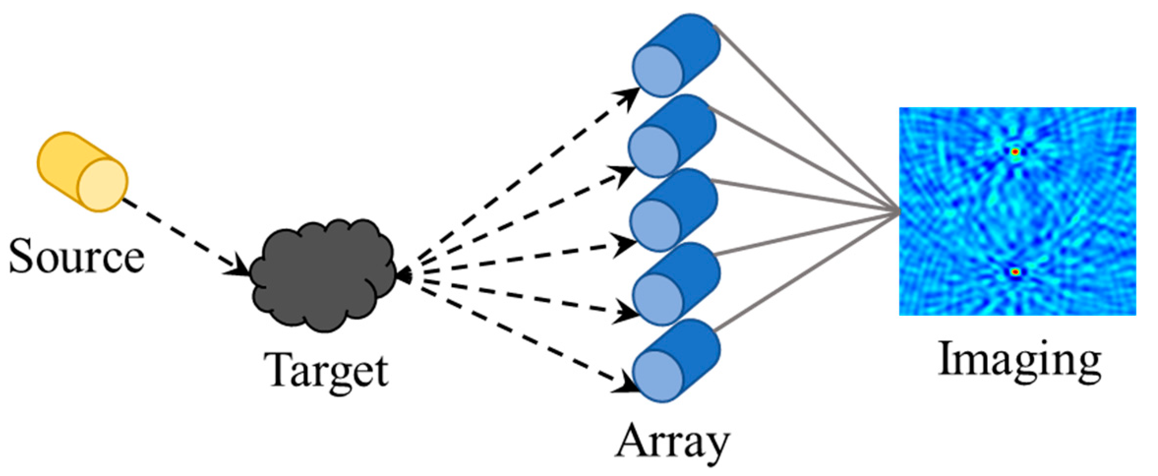
2.1. Synthetic Aperture Sonar Imaging Model

Firstly, a typical underwater SAS imaging model is given in Figure 1. In the imaging model, the sonar source emits acoustic waves to the target, and the arrays receive the echo waves reflected by the underwater target. Besides, the obtained reflected signal waves are processed by the imaging algorithm, and the acoustic imaging of the underwater target is outputted.

Here, the physical spatial resolution of the underwater target in the final acoustic imaging is the primary focus of this study. The emitting process is affected by several important parameters, which could be concluded by:

$$H_{st}(S_f,A_s,P_{st}),$$

(1)

where, $S_f$ is the frequency of the emitting signal, $A_s$ is the amplitude of the emitting signal, and $P_{st}$ is the path that acoustic waves travel from the source to the target. Similarly, the receiving process is concluded by:

$$H_{ta}(S_f,D_t,P_{ta}),$$

(2)

where, $S_f$ is the frequency of the emitting signal, $D_t$ is the target features (i.e., size, shape, and material) that impact the echo waves, $P_{ta}$ is the path that acoustic waves travel from the target to the array. The final acoustic imaging and the physical spatial resolution of the underwater target are determined by:

$$F(H_{st},H_{ta},L_x,L_y,N_a),$$

(3)

where, $H_{st}$ and $H_{ta}$ are the emitting and receiving process. $L_x$ and $L_y$ are the aperture of the array in x and y direction. $N_a$ is the number of elements in the array. The $F\left(•\right)$ is the imaging algorithm. The $H_{st}$ and $H_{ta}$ mainly influence the reflected signal wave, and the frequency of the signal waves is a great factor that influences the physical spatial resolution of the underwater target. In addition, the aperture of the array is another significant parameter that affects the final resolution. A larger aperture would lead to high-resolution and a smaller spot. The $N_a$ mainly affects the amplitude and signal-to-noise ratio of the target imaging, which is another essential aspect to reveal the performance of the imaging system.

In this work, the delay and sum (DAS) algorithm is used to image the underwater target with the reflected signal waves received by the sonar array. The DAS is a kind of coherent superposition method in synthetic aperture. Based on the relationship between travel distance and wave velocity, the coherent superposition of the whole elements is calculated on every pixel in the imaging area, where the reconstruction process of pixel i could be expressed as:

$$I(x,z)={\displaystyle \sum _{i=1}^n{S}_i(t_i)},$$

(4)

where, $S_i(•)$ is the pretreated signal wave received by each array element. $t_i$ are the corresponding time taken from transmission to reception. The data preprocessing includes filtering and pulse compression. $t_i$ are calculated by the travel distance and wave velocity. The final acoustic image is obtained by calculating all the pixels in the imaging area through Equation (4).

2.2. The End-to-End Neural Networks

The deep learning method is applied to improve the physical spatial resolution of underwater targets in the final acoustic imaging. Here, a U-shaped convolutional neural network is employed for the purpose of achieving super-resolution. The construction of the crafted end-to-end neural network is shown in Figure 2.

The end-to-end neural network consists of two parts: the down-sampling part and the up-sampling part. The input low-resolution images are encoded into feature vectors by three down-sampling layers, then the feature vectors are extended to the high-resolution through three up-sampling layers. Various features extracted by each down-sampling layer are copied and cropped to the corresponding up-sampling layer to maintain prior knowledge of input imaging and accelerate convergence speed.

The down-sampling layer contains two convolution blocks and a 2D max pooling layer. The convolution block is composed of a 2D convolution layer, a batch normalized layer, and a ReLU activation function. The three down-sampling layers are utilized to extract features from the initial images characterized by low physical spatial resolution. Subsequently, these extracted features are reshaped into vectors for further analysis. Meanwhile, the up-sampling layer contains a 2D transposed convolution layer and a concatenating layer. The concatenating layer copied and cropped the features extracted by the corresponding down-sampling layer. The 2D transposed convolution layers gradually transform the feature vectors into high-resolution imaging.

In the domain of sonar image processing, this end-to-end neural network effectively tackles the dual challenges of low resolution and intrinsic noise characteristic of such imagery. It significantly improves both the quality and interpretability of these images, demonstrating exceptional efficacy in underwater target detection and classification tasks. Leveraging an end-to-end training paradigm, the network autonomously learns the mapping from raw sonar images to their high-resolution versions, thereby eliminating the need for manual feature engineering and enhancing the system’s robustness and generalizability. This approach not only streamlines the processing pipeline but also ensures more reliable and adaptable performance in diverse underwater environments.

In the training phase, the end-to-end neural network learns the mapping function $M_{\theta }$ from a large amount of labeled data $(y_i,x_i),i=1,\dots ,n$ by solving:

$$I(x,z)={\displaystyle \sum _{i=1}^n{S}_i(t_i)},$$

(5)

where, $M_{\theta }$ is the mapping function of the neural network defined by a set of weights and biases $\theta \in \Theta$. N is the number of training samples. $y_i$ are the input low-resolution images and $x_i$ are the corresponding high physical spatial resolution images. We focus on enhancing the resolution reduction due to the limited aperture, i.e., the $L_x$ and $L_y$ in Equation (3).

2.3. The Construction of Simulated Dataset

Simulations are conducted to generate the data sets used for network training and testing. Linear frequency modulation signal waves with 70 kHz–100 kHz are emitted with the sonar source. The sonar source and array are set on the water surface, and the target is located underwater 20 m. Targets in the simulations are the corresponding consistent point target in each direction. The rounded receiving sonar array contains 256 elements. The radius of the array is set to 1.4 m to generate the low physical spatial resolution images. Besides, we expand the radius of the array to 4.2 m to simulate the case of high physical spatial resolution images achieved by a large aperture, which is illustrated in Figure 3. Hence, the labeled samples are realized, which corresponds to the reduction of physical resolution due to the limited aperture in practice.

We consider the case of a single target firstly, that is, there is only one target in the imaging area. The end-to-end neural network attempts to enhance the physical spatial resolution of the target in the sonar images. Specifically, the trained network would learn the projection from the limited aperture, low-resolution to large aperture, high-resolution. 1000 simulations are realized to generate the data sets, in which 800 samples are used in the training phase and 200 samples are applied in testing. The training set is independent of the testing set, that is, there is no iterative sample in two data sets. Figure 4 gives a clear look at the samples. Due to the aperture size, we can see the reduction of physical spatial resolution in Figure 4a, which demonstrates in larger target size and sidelobe.

The samples are pre-processed before being fed into the neural network. The preprocessing includes data normalization, logarithmic processing, and random order disruption. Usually, these steps could speed up the convergence of the network and optimize generalization performance.

In the training phase, the batch size is set to 20, and the network is trained for 100 epochs. The root mean square prop optimizer with a learning rate of 5 × 10⁻⁴, the momentum of 0.9, and weight decay of 1 × 10⁻⁸ is used to train the end-to-end network. The weights and biases of the proposed network are updated by the propagation of root mean square errors between the predicted high-resolution imaging and the ground truth.

In this study, all computational algorithms were implemented and executed utilizing MATLAB R2023a, operating within the Windows 11 environment.

3. Results and Discussion

3.1. Resolution Enhancing in the Single Target Case

The normalized loss curve is plotted in Figure 5. With the increase of the training epochs, the normalized loss on the whole test set gradually declines. When the epoch grows to 20, the normalized loss on the test set declines to 1 × 10⁻⁴. The normalized loss future reduces below 5 × 10⁻⁴ after finishing 100 epochs of training. The loss curve indicates that the end-to-end network is well trained and performs greatly on the entire test set.

Without loss of generality, we randomly select one testing sample to show the performance of the network. The predicted high-resolution imaging outputted by the trained network and the ground truth are shown in Figure 6a,b. One can see great visual agreement between the predicted result and the true high-resolution imaging, whether the resolution of the target or its intensity. Compared with the inputted low-resolution imaging established in Figure 6c, the resolution of the target in both directions is improved significantly.

The normalized maximum amplitude of Figure 6a,b in x and y directions are plotted in Figure 7 to reveal the difference between the network predicted high-resolution imaging and the real high-resolution imaging more clearly. Among them, x and y denote the floating-point numerical values associated with their respective directional components. The predicted profiles in Figure 7 are highly similar to the true ones. The tiny differences mainly occur in the amplitude at the top of the profiles, which have little effect on the determination of target resolution. The profiles in Figure 7 show that the network achieves the improvement of target resolution, while accurately preserving the position of the target, intensity distribution, and other important information.

An attempt is made to further enhance the resolution of the target, thereby pushing it to its theoretical limit (the impulse function of the target). The impulse function of the target is the impulse located at the target position and valued at 1. Usually, the impulse function of the target is the limitation of the physical spatial resolution, which contains the ideal target response of the imaging system. Based on the predicted high-resolution imaging, we use the same network structure to reconstruct the mapping from the high-resolution imaging to the impulse function of the target.

The configuration of datasets is the same as the above. 800 samples are used for training, meanwhile, 200 samples are used for testing. Similarly, a 100-epoch training is conducted, and the trained network performs greatly in the whole test set. A random testing sample is selected to show the perdition results. The predicted impulse function of the target, the ground truth of the impulse function, and the inputted high-resolution imaging are given in Figure 8. The predicted impulse function of the target is highly consistent with the ground truth, whether the location or amplitude of the target. The physical spatial resolution is future enhanced to the limitation compared with the inputted high-resolution imaging in Figure 8c.

To compare the details of Figure 8a,b, the normalized maximum amplitude at x and y directions are displayed in Figure 9. Even in both directions, the theoretical impulse response is only one pixel wide, and the outputted impulse function of the target is total consistency with theoretical results in the distribution. The results could help us detect and locate targets in case of limited aperture due to various reasons in practice.

3.2. Resolution Enhancing in the Multiple Targets Case

Although the end-to-end network performs well in the single-target case, more complex cases should be considered. We future focus on the case of multiple targets. Serval (1–3) point targets are randomly placed in the imaging area to simulate the case of multiple targets. The uncertain target number and the interaction between each target make it changeling to improve the physical spatial resolution of every target one time. The configuration of the training and testing set is the same as the single target case, and the proposed neural network is trained for 100 epochs.

The normalized loss curve of multiple targets case is plotted in Figure 10. The normalized loss on the whole test set declines rapidly as the number of training epochs increases. After 20 epochs of training, the normalized loss is already less than 1 × 10⁻⁴. The normalized loss future declined to less than 1 × 10⁻⁵ after 100 epochs of training. The results present that the end-to-end network is able to improve the physical spatial resolution of multiple targets case.

A three targets sample is randomly picked up to take a close look at the predicted results and the ground truth. The predicted high-resolution imaging, the ground truth of high-resolution imaging, and the inputted low-resolution imaging in multiple targets case are given in Figure 11. Compared with the inputted low-resolution imaging Figure 11c, The resolution predicted target imaging is greatly enhanced in both directions while maintaining the right target location and amplitude. Moreover, the predicted high-resolution result is highly consistent with the theoretical high-resolution result in target number, location, and amplitude, which demonstrates that the trained end-to-end network performs precisely in the task of multi-target resolution enhancement.

The normalized maximum amplitudes at the x and y direction of Figure 11a,b are shown in Figure 12. It can be seen more clearly that the result of network prediction is affirmed adjacent to the theoretical ones. The significant features that the coordinate and amplitude of each target are well preserved, in which the coordinate reveals the location of the target while the amplitude reveals the interaction with the other targets.

We extend our analysis to future improve the resolution of the target. Consistent with the findings, our objective is to push the physical resolution to its utmost limit. In other words, to transform multiple targets to the impulse responses in corresponding position simultaneously. The end-to-end network is retrained to fit the mapping from the obtained high-resolution imaging to the impulse response in multiple targets cases. The training strategy and dataset setting are the same as the above. The detailed prediction result, the ground truth of impulse function, and the inputted high-resolution imaging are listed in Figure 13. The predicted impulse functions for multiple targets exhibit a high degree of similarity to the ground truth data. There was no shift in target position or decrease in some target resolution due to the increase in the number of targets. The results show that the proposed network could further compress the targets in high-resolution imaging to the extreme resolution, even in the multiple targets case.

It can be seen from the normalized maximum amplitudes at the x and y direction illustrated in Figure 14 that the predicted impulse function of the multiple targets differs fractionally to the theoretical results in both amplitude and coordinate of every target, which is consistent with the Figure 13a,b. The results demonstrated herein indicate that the proposed network significantly enhances imaging resolution, even extending the boundaries of the physical spatial resolution constraints inherent in underwater multi-target imaging systems. This is of great significance for underwater target recognition and feature extraction.

4. Conclusions

In this work, the deep learning method is utilized to enhance the physical spatial resolution of sonar images with underwater targets. An end-to-end neural network that contains the down-sampling part, up-sampling part, and the skip connections to map an inputted low-resolution imaging to an outputted high-resolution imaging. The physical spatial resolution enhancement attributable to the limited array aperture is examined, with two scenarios investigated: the single target case and the multiple target cases. The loss curves indicate that the normalized loss on the testing set declines significantly in both cases with the increase of the training epoch. After 100 epochs of training, the network could predict precise high-resolution imaging with an uncertain target number. An additional effort is undertaken to reconstruct the predicted high-resolution imaging to its physical spatial resolution target utilizing the identical network structure. The results indicate that the network could trend the high-resolution target to its theoretical impulse response at the same location and amplitude. In conclusion, the present end-to-end neural network performs well in the task of improving the resolution of underwater targets in sonar images and broadens the application of deep learning in sonar image enhancement.

References

1. Hayes, M.P.; Gough, P.T. Synthetic aperture sonar: A review of current status. IEEE J. Ocean. Eng. 2009, 34, 207–224. [Google Scholar] [CrossRef]
2. Ning, M.; Zhong, H.; Tang, J.; Wu, H.; Zhang, J.; Zhang, P.; Ma, M. A Novel Chirp-Z Transform Algorithm for Multi-Receiver Synthetic Aperture Sonar Based on Range Frequency Division. Remote Sens. 2024, 16, 3265. [Google Scholar] [CrossRef]
3. Zhang, J.; Cheng, G.; Tang, J.; Wu, H.; Tian, Z. A Subaperture Motion Compensation Algorithm for Wide-Beam, Multiple-Receiver SAS Systems. J. Mar. Sci. Eng. 2023, 11, 1627. [Google Scholar] [CrossRef]
4. Marston, M.T.; Hall, R.B.; Bassett, C.; Plotnick, D.S.; Kidwell, A.N. Motion tracking of fish and bubble clouds in synthetic aperture sonar data. J. Acoust. Soc. Am. 2024, 155, 2181–2191. [Google Scholar] [CrossRef]
5. Zhang, X.; Heald, G.; Lyons, P.A.; Hansen, R.E.; Hunter, A.J. Guest editorial: Recent advances in synthetic aperture sonar technology. Electron. Lett. 2023, 59, e12881. [Google Scholar] [CrossRef]
6. Cheng, J.; Ge, J.; Bai, R. Enhanced Multi-Beam Echo Sounder Simulation through Distance-Aided and Height-Aided Sound Ray Marching Algorithms. J. Mar. Sci. Eng. 2024, 12, 913. [Google Scholar] [CrossRef]
7. Wei, B.; Zhou, T.; Li, H.; Xing, T.; Li, Y. Theoretical and experimental study on multibeam synthetic aperture sonar. J. Acoust. Soc. Am. 2019, 145, 3177–3189. [Google Scholar] [CrossRef] [PubMed]
8. Myers, V.L.; Sternlicht, D.D.; Lyons, A.P.; Hansen, R.E. Automated seabed change detection using synthetic aperture sonar: Current and future directions. In Proceedings of the International Conference on Synthetic Aperture Sonar and Synthetic Aperture Radar, Lerici, Italy, 17–19 September 2014; pp. 1–10. [Google Scholar]
9. Gupta, K.S.; Chauhan, S.C.R.; Kumar, V. Channel modelling in underwater media: A wireless communication technique perspective. Phys. Scr. 2024, 99, 112003. [Google Scholar] [CrossRef]
10. Wan, L.; Deng, S.; Chen, Y.; Cheng, E. Sparse channel estimation for underwater acoustic OFDM systems with super-nested pilot design. Signal Process. 2025, 227, 109709. [Google Scholar] [CrossRef]
11. Xiang, D.; He, D.; Wang, H.; Qu, Q.; Shan, C.; Zhu, X.; Zhong, J.; Gao, P. Attenuated color channel adaptive correction and bilateral weight fusion for underwater image enhancement. Opt. Lasers Eng. 2025, 184, 108575. [Google Scholar] [CrossRef]
12. Ji, M.; Ren, G.; Liu, J.; Xu, Q.; Ren, R. Multi-person cooperative positioning of forest rescuers based on inertial navigation system (INS), global navigation satellite system (GNSS), and ZigBee. Measurement 2025, 241, 115669. [Google Scholar] [CrossRef]
13. Sutton, T.J.; Griffiths, H.D.; Hetet, A.P.; Perrot, Y.; Chapman, S.A. Experimental validation of autofocus algorithms for high-resolution imaging of the seabed using synthetic aperture sonar. IEE Proc.-Radar Sonar Navig. 2003, 150, 78–83. [Google Scholar] [CrossRef]
14. Zhao, F.; Mizuno, K.; Tabeta, S.; Hayami, H.; Fujimoto, Y.; Shimada, T. Survey of freshwater mussels using high-resolution acoustic imaging sonar and deep learning-based object detection in Lake Izunuma, Japan. Aquat. Conserv. Mar. Freshw. Ecosyst. 2023, 34, e4040. [Google Scholar] [CrossRef]
15. Sung, M.; Joe, H.; Kim, J.; Yu, S.C. Convolutional Neural Network Based Resolution Enhancement of Underwater Sonar Image Without Losing Working Range of Sonar Sensors. In Proceedings of the 2018 OCEANS-MTS/IEEE Kobe Techno-Oceans (OTO), Kobe, Japan, 28–31 May 2018; pp. 1–6. [Google Scholar]
16. Sung, M.; Kim, J.; Yu, S.C. Image-based Super Resolution of Underwater Sonar Images using Generative Adversarial Network. In Proceedings of the TENCON 2018-2018 IEEE Region 10 Conference, Jeju, Republic of Korea, 28–31 October 2018; pp. 0457–0461. [Google Scholar]
17. Islam, M.J.; Enan, S.S.; Luo, P.; Sattar, J. Underwater Image Super-Resolution using Deep Residual Multipliers. In Proceedings of the 2020 IEEE International Conference on Robotics and Automation (ICRA), Paris, France, 31 May–31 August 2020; pp. 900–906. [Google Scholar]
18. Xu, P.; Xu, S.; Shi, K.; Ou, M.; Zhu, H.; Xu, G.; Gao, D.; Li, G.; Zhao, Y. Prediction of Water Temperature Based on Graph Neural Network in a Small-Scale Observation via Coastal Acoustic Tomography. Remote Sens. 2024, 16, 646. [Google Scholar] [CrossRef]
19. Zang, X.; Yin, T.; Hou, Z.; Mueller, R.P.; Deng, Z.D.; Jacobson, P.T. Deep Learning for Automated Detection and Identification of Migrating American Eel Anguilla rostrata from Imaging Sonar Data. Remote Sens. 2021, 13, 2671. [Google Scholar] [CrossRef]
20. Qiao, J.; Li, D.; Zheng, M.; Liu, Z.; Yang, H. Neural network-based adaptive tracking control for denitrification and aeration processes with time delays. IEEE Trans. Neural Netw. Learn. Syst. 2024, 35, 15507–15516. [Google Scholar] [CrossRef] [PubMed]
21. Dao, P.N.; Phung, M.H. Nonlinear robust integral based actor–critic reinforcement learning control for a perturbed three-wheeled mobile robot with mecanum wheels. Comput. Electr. Eng. 2025, 121, 109870. [Google Scholar] [CrossRef]
22. Christensen, H.J.; Mogensen, V.L.; Ravn, O. Side-Scan Sonar Imaging: Real-Time Acoustic Streaming. IFAC-Pap. 2021, 54, 458–463. [Google Scholar] [CrossRef]
23. Sung, M.; Kim, J.; Lee, M.; Kim, B.; Kim, T.; Kim, J.; Yu, S. Realistic Sonar Image Simulation Using Deep Learning for Underwater Object Detection. Int. J. Control. Autom. Syst. 2020, 18, 523–534. [Google Scholar] [CrossRef]
24. Haahr, J.C.; Valdemar, L.M.; Ravn, O. Deep Learning based Segmentation of Fish in Noisy Forward Looking MBES Images. IFAC-Pap. 2020, 53, 14546–14551. [Google Scholar]
25. Cui, H.; Zhao, W.; Wang, Y.; Fan, Y.; Qiu, L.; Zhu, K. Improving spatial resolution of confocal raman microscopy by super-resolution image restoration. Opt. Express 2016, 24, 10767–10776. [Google Scholar] [CrossRef] [PubMed]
26. Pacifici, F.; Longbotham, N.; Emery, W.J. The Importance of Physical Quantities for the Analysis of Multitemporal and Multiangular Optical Very High Spatial Resolution Images. IEEE Trans. Geosci. Remote Sens. 2014, 52, 6241–6256. [Google Scholar] [CrossRef]
27. Alvaro, V.; Karin, R.; Simon, J. A new metric for the assessment of spatial resolution in satellite imagers. Int. J. Appl. Earth Obs. Geoinf. 2022, 114, 103051. [Google Scholar]
28. Xu, J.; Zhang, P.; Chen, Y. Surface Plasmon Resonance Biosensors: A Review of Molecular Imaging with High Spatial Resolution. Biosensors 2024, 14, 84. [Google Scholar] [CrossRef]
29. Su, Y.; Chen, X.; Cang, C.; Li, F.; Rao, P. A Space Target Detection Method Based on Spatial–Temporal Local Registration in Complicated Backgrounds. Remote Sens. 2024, 16, 669. [Google Scholar] [CrossRef]
Figure 1. The typical synthetic aperture sonar imaging model.
Jmse 13 00134 g001
Figure 2. The construction of the end-to-end neural network.
Jmse 13 00134 g002
Figure 3. The sonar array with the limited and large aperture.
Jmse 13 00134 g003
Figure 4. The (a) low-resolution samples and (b) corresponding high-resolution samples.
Jmse 13 00134 g004
Figure 5. The loss curve of the single target case.
Jmse 13 00134 g005
Figure 6. (a) The predicted high-resolution imaging, (b) the ground truth of high-resolution imaging, and (c) the inputted low-resolution imaging.
Jmse 13 00134 g006
Figure 7. The normalized maximum amplitude in (a) x direction and (b) y direction.
Jmse 13 00134 g007
Figure 8. (a) The predicted impulse function of the target, (b) the ground truth of impulse function, and (c) the inputted high-resolution imaging.
Jmse 13 00134 g008
Figure 9. The normalized maximum amplitude in (a) x direction and (b) y direction.
Jmse 13 00134 g009
Figure 10. The loss curve of the multiple targets case.
Jmse 13 00134 g010
Figure 11. (a) The predicted high-resolution imaging, (b) the ground truth of high-resolution imaging and (c) the inputted low-resolution imaging.
Jmse 13 00134 g011
Figure 12. The normalized maximum amplitude in (a) x direction and (b) y direction.
Jmse 13 00134 g012
Figure 13. (a) The predicted impulse function of the multiple targets, (b) the ground truth of impulse function and (c) the inputted high-resolution imaging.
Jmse 13 00134 g013
Figure 14. The normalized maximum amplitude at (a) x direction and (b) y direction.
Jmse 13 00134 g014
Disclaimer/Publisher’s Note: The statements, opinions and data contained in all publications are solely those of the individual author(s) and contributor(s) and not of MDPI and/or the editor(s). MDPI and/or the editor(s) disclaim responsibility for any injury to people or property resulting from any ideas, methods, instructions or products referred to in the content.