Article

Cyclic Peak Extraction from a Spatial Likelihood Map for Multi-Array Multi-Target Bearing-Only Localization

1
State Key Laboratory of Acoustics, Institute of Acoustics, Chinese Academy of Sciences, Beijing 100190, China
2
College of Physical Sciences, University of Chinese Academy of Sciences, Beijing 100049, China
*
Author to whom correspondence should be addressed.
J. Mar. Sci. Eng. 2025, 13(1), 109; https://doi.org/10.3390/jmse13010109
Submission received: 24 December 2024 / Revised: 4 January 2025 / Accepted: 6 January 2025 / Published: 8 January 2025
(This article belongs to the Section Ocean Engineering)

Abstract

:
In the context of multi-array multi-target bearing-only localization, due to the existence of direction-finding errors, the crossing results of bearing lines cannot accurately determine correspondence with targets. Under conditions that clutter interference and missing of detection in direction-finding, the traditional method will produce false alarm targets and miss some targets. To address this issue, this paper draws on the idea of a spatial likelihood map which calculates the likelihood of target presence at each grid point within the observation area by partitioning the observation area into grids and utilizing bearing data from each array, yielding the distribution of targets in the observation area. Then, a multi-target cyclic peak extraction algorithm based on a statistical dual-threshold is proposed, which eliminates false peaks by cyclic extraction of target positions, so as to reduce false targets. Simulation results demonstrate that the spatial likelihood mapping-based localization exhibits good performance. Furthermore, when the multi-target cyclic peak extraction algorithm based on statistical dual-thresholds is applied, it outperforms direct target extraction from the spatial likelihood map, showcasing enhanced multi-target localization capabilities. Moreover, compared to the position non-linear least squares multi-target localization method, the proposed method has lower optimal sub-pattern assignment distance and lower localization error under the condition of interference and missing detection.

1. Introduction

The bearing-only localization problem has been studied for decades [1], and the methods developed for it are widely applied in radar and sonar systems [2,3,4]. In a bearing-only localization scenario, the target’s position is estimated by intersecting bearing lines obtained from multiple different arrays or mobile observation stations. A sensor network refers to a network of sonar arrays, or nodes, arranged according to a specific pattern in the underwater environment [5]. By integrating the data received from multiple nodes, target localization and tracking can be achieved [6,7].
There has been considerable research on the multi-array bearing-only localization problem for a single target, which can be broadly categorized into two types. The first type is Maximum Likelihood Estimation (MLE) [8]. Under the assumption of Gaussian noise, MLE is similar to the nonlinear least squares (NLSs) method and is equivalent to estimating the target’s position by solving a nonlinear least squares optimization problem. The cost function of this optimization problem is defined by the sum of squared errors between the direction-of-arrival (DOA) estimates and the unknown true DOA values at all sensor nodes. Due to the nonlinear and non-convex nature of this method, the MLE problem needs to be solved iteratively, requiring a good initial estimate to avoid convergence to a local minimum. Additionally, under conditions of low signal-to-noise ratio (SNR) and poor geometry [9], iterative methods may become unstable and prone to divergence. The second type involves closed-form solutions, which generally have lower computational complexity. Stansfield [10] proposed a weighted linear least squares estimator by linearizing the NLS cost function. This method has the advantage of high computational efficiency, but the resulting pseudo-linear estimator increases the estimation bias. The total least squares method based on orthogonal vectors [11] is also relatively easy to implement. Compared to the pseudo-linear estimator, this method reduces the estimation bias in the presence of azimuth noise and sensor position errors. Additionally, methods such as auxiliary variables [12] and constrained least squares [13] can reduce bias and are asymptotically unbiased. Another approach is the intersection-point (IP) method [14], which estimates the target position by calculating the centroid of the intersection points of the bearing lines (DOA lines). Similar to the pseudo-linear estimator, the IP method also introduces estimation bias. Grid-based methods [15] achieve the same accuracy as that of the NLS estimator, do not require a good initial estimate, and reduce the computational burden of the minimization process, though they necessitate the selection of an appropriate grid width.
The solutions discussed above are primarily for single-target localization. When multiple targets are present in the observation area, the problem becomes more complex. The main difficulty lies in data association, as the direction-of-arrival (DOA) estimates from multiple nodes cannot be definitively matched with specific targets. Incorrect associations lead to the generation of false targets. To address this, combinatorial methods can be employed to identify the combination with the minimum cost. However, as the number of nodes and targets increases, this approach results in extremely high computational complexity, making it an NP-hard problem, which is not suitable for real-time applications. Currently, several methods have been proposed to solve the data association problem [16,17], including approaches based on clustering of intersection points of bearing lines [18], among others. However, many of these methods do not account for the adverse effects of missed detections or false alarms. Even when these factors are considered, the computational complexity remains high in scenarios with multiple nodes and targets.
Constructing a spatial likelihood map to model the target distribution is a direct method for target position estimation. Existing approaches based on spatial correlation fields [19,20], Steered Response Power (SRP) [21,22,23], and multi-node spatial likelihood weighted sums [24] estimate the target position by locating the peak of the spatial likelihood map. Omologo [19] locates the sound source position by analyzing the phase difference of the cross-power spectrum. Brutti [20] exhibits high localization accuracy under reverberant conditions. Huang [21] considers band-pass signals related to the uncertainty of the steering delay and a coarser spatial grid, demonstrating superior performance in outdoor environments. Do [22] reduces computational cost by iteratively narrowing the search area and evaluating function values on a coarse grid while maintaining localization accuracy. Cobos [23] comprehensively explores the sampling space by calculating the SRP across the entire space, rather than just at discrete spatial locations, thereby enhancing robustness and allowing for the use of a rougher spatial grid. Aarabi [24] utilizes the Spatial Likelihood Function (SLF) generated by each microphone array, and sums them through a weighted summation approach. Some works [25] sequentially estimate the strongest peaks in the likelihood map and then remove their contributions from the map until all targets are identified. However, as the number of targets increases, the likelihood map tends to exhibit multiple local maxima, some of which correspond to false targets, thereby reducing the method’s performance.
In this paper, to improve the performance of multi-array bearing-only target localization estimation, we propose an improved approach for constructing the likelihood map by incorporating intersection points and bearing lines. This method avoids the high computational complexity of data association and extracts targets from the likelihood map using a statistical dual-threshold approach, ultimately enhancing the multi-array bearing-only localization capability. Compared to traditional methods, the method proposed in this paper exhibits higher localization capability in the presence of interference and missed detections.
The following is the main structure of this paper. Section 1 is the introduction. Section 2 is the mathematical model and theoretical framework. Section 3 discusses the principle of bearing-only localization algorithm based on spatial likelihood map. Section 4 is the simulation. And Section 5 is the conclusion and discussion.

2. Mathematical Model and Theoretical Framework

The sensor network consists of multiple nodes, with each node corresponding to a sonar array. Each array is responsible for receiving the sound source signals in the observation area and estimating the direction-of-arrival (DOA) of the received signals. The position coordinates of each array are assumed to be known, and by performing bearing-crossing localization using the DOA estimates from different arrays, the position of the sound source can be determined.
Assume that the number of nodes (i.e., the number of arrays) is M , and the 2D coordinates (the two-dimensional plane is only considered in this paper) of the m -th node are denoted as q m :
q x , m q y , m T ,
The number of sound sources is N , and the 2D coordinates of the n -th sound source are denoted as p n :
p x , n p y , n T ,
The positions of all sound sources are represented as
P = p 1 p 2 p n p N T ,
The DOA (this angle is measured from the east direction, rotating counterclockwise) of the n -th sound source relative to the m -th node is denoted as
θ m p n = arctan p y , n q y , m p x , n q x , m ,
The observation results are represented as
θ ^ m , n = θ m p n + w m , n ,
where w m , n is the observation noise for the DOA measurement of the n -th target at the m -th node, and w m , n is assumed to follow a zero-mean Gaussian distribution with variance σ m , n 2 . Let the m -th node have S m bearing measurements, and the observed angle vector is denoted as:
θ ^ m p = θ ^ m , 1 θ ^ m , 2 θ ^ m , s θ ^ m , S m T
When there is only one target in the observation area, the sound source coordinate p is represented as p x p y T .
A simpler direct method for single-target localization is the least squares (LSs) method [8,11]. Let the measurement data of the m -th node be θ ^ m . Assuming the target lies on the bearing line corresponding to this measured angle,
p x sin θ ^ m p y cos θ ^ m = q x , m sin θ ^ m q y , m cos θ ^ m ,
By combining the data from M nodes, the following system of linear equations can be obtained:
E p = b ,
where E = sin θ ^ 1 cos θ ^ 1 sin θ ^ M cos θ ^ M   b = q x , 1 sin θ ^ 1 q y , 1 cos θ ^ 1 q x , M sin θ ^ M q y , M cos θ ^ M .
Due to the presence of observational errors, the system of equations does not have an exact solution. Using linear least squares (LLSs) [8,11], the estimated target position can be obtained by minimizing the sum of squared errors:
p ^ L L S = A T A 1 A T b ,
When the observation errors at all nodes have the same distribution, nonlinear least squares (NLSs) is equivalent to Maximum Likelihood Estimation (MLE) [8]. This method aims to find the position coordinates p ^ N L S that minimize the following cost function:
p ^ N L S = argmin p m = 1 M θ ^ m θ m p 2 ,
Using the solution from linear least squares (LLSs) as the initial value, the minimization problem can be solved using Recursive Gradient Descent.
In the Intersection Point (IP) method, the target position is estimated by calculating the centroid of all intersection points of the bearing lines. To increase accuracy, large-error intersection points can be discarded. This method can be considered a suboptimal solution to the linear least squares (LLSs) problem [14].
The Grid-Based (GB) method [15] involves searching over a grid of potential target locations and selecting the grid point n that minimizes the cost function, typically the sum of squared errors between the observed and predicted DOA values. The estimated target position is then given by the grid point that satisfies the following condition:
n * = argmin n m = 1 M A θ ^ m , Ψ m , n 2 ,
where Ψ m , n is the DOA data of the m -th node relative to the n -th grid point, and A ( X , Y ) is denotes as:
A X , Y = min X Y m o d   2 π , Y X m o d   2 π ,
The above discussion focused on the single-target scenario. For multi-target situations, most existing multi-sensor bearing-only localization methods involve assigning measurement data to different targets, calculating the cost function for each assignment, and selecting the assignment that minimizes the cost function. The target positions are then estimated using single-target methods. Various optimization algorithms have been proposed to solve this assignment problem [26,27]. However, when the number of targets increases or the number of sensors grows, these algorithms cannot be processed in real-time. To address this issue, constructing a spatial likelihood map based on target distribution probabilities is one potential solution. However, existing methods have not fully resolved this problem [19,20,21,22,23,24,25]. In this paper, we propose an improvement on the construction of the spatial likelihood map and use a multi-target extraction method based on statistical dual-threshold for the cyclic extraction of targets, allowing for the localization of a larger number of targets.
For ease of discussion, the following parameters are defined for the simulation:
  • Number of Targets, N . Targets are randomly placed within the observation area, with their positions following a uniform distribution. To ensure that the targets are sufficiently spaced for clarity, the distance between any two targets is greater than D m i n = 700   m .
  • Target-Bearing Detection Probability, P d , m . Each sensor has a probability of detecting each target. This detection probability is modeled as a detection rate. When generating bearing information for a target, the system first checks if the target is detected. If detected, the bearing measurement is generated with Gaussian distribution errors. In the underwater environment, the detection probability can be modeled using a probability perception model [28,29]:
    P d , m n = e α · Δ m n ,
    where n represents a location in the observation area. α is the attenuation coefficient of sensor m ’s detection ability. Δ m n is the distance between the sensor m and location n . When the target reaches the maximum detection range of the sensor Δ m , m a x , the detection probability is 0.5. Therefore, α = l n 2 Δ m , m a x .
  • Expectation of Interference Number, u . In addition to detecting true target bearings, each sensor may also produce several false bearing measurements, referred to as interference. These interferences may result from environmental or system noise. When the interference sources are uniformly distributed, and the occurrence probability of interference is independent of space and time, a Poisson distribution is used to model the number of interference sources within a given spatial range. The number of interferences x u follows a Poisson distribution with parameter u , i.e., P x u = k = e u u k k ! . Each interference is assumed to be uniformly distributed within the sensor’s bearing observation range.

3. Principle of Bearing-Only Localization Algorithm Based on Spatial Likelihood Map

The sensor network used in this paper consists of four nodes located at the corners of a square boundary, as shown in Figure 1. The observation area is the interior of the square, enclosed by the nodes. The targets are randomly distributed within the observation area, with the number of targets being unknown. It is assumed that the DOA observation errors for each node follow the same Gaussian distribution with a mean of 0 and a variance of σ θ 2 .
We divide the observation area into a grid, with all grid points described by Σ , and the grid width denoted as G . The spatial likelihood map M ( n , t ) represents the probability of a sound source existing at position n Σ at time t . This map is also referred to as the source distribution ambiguity map. Under ideal conditions, the actual target source location corresponds to the global maximum value in the spatial likelihood map. Therefore, the position of the global maximum peak in the spatial likelihood map can be used as the estimated target location:
n ^ = argmax n Σ M n ,
Since we are dealing with a localization problem at a single time instant, for simplicity we remove the time dependency from the notation. The position estimation error introduced by spatial discretization can be described as [15]:
E G B = V 6 N g 1 ,
where V is the side length of the observation area, and N g is the total number of grid points. To obtain effective estimation results, the spatial discretization error needs to be sufficiently small. Under the condition that the side length V of the region is fixed, increasing the number of grid points N g can reduce this error. However, this also increases the computational burden, so the grid partitioning of the region must be carefully balanced.
In cases where all arrays are capable of observing the target, large errors in the bearing angle from a particular array can lead to significant localization errors using the aforementioned single-target localization methods. The use of a spatial likelihood map for localization helps mitigate this issue by incorporating data from multiple arrays. There are two main approaches for multi-array bearing-based target localization. The first is Intersection Point Estimation, and the second is Bearing Angle Deviation Estimation. Both of these methods rely on the assumption that the bearing measurement errors follow a Gaussian distribution.
For the l -th bearing line (denoted as bearing l 1 from array i 1 ), which represents the bearing angle from a specific array, once the bearing measurement is obtained, we assume it corresponds to a real target. The true target corresponding to this bearing would satisfy a Gaussian distribution with the mean of the bearing angle measurement and variance σ θ 2 . Given the bearing lines alone, for any grid point n in the observation area, the relative bearing angle from array i 1 is denoted as Ψ i 1 , n . The likelihood probability of a target existing at the grid point n , when corresponding to the bearing line l 1 of array i 1 , is given by:
Λ l n = P i 1 , l 1 n ,
where P i 1 , l 1 n represents the likelihood probability of grid point n relative to the bearing line l 1 of array i 1 . It follows a Gaussian distribution with mean A θ ^ i 1 , l 1 , Ψ i 1 , n and variance σ θ 2 , where A is defined by Equation (12), and θ ^ i 1 , l 1 is the bearing measurement from the l 1 -th bearing line of array i 1 . Since the bearing error is assumed to be Gaussian, and given the measurement result, the true bearing of the target corresponds to the Gaussian distribution centered at the measurement. Therefore, for each array, the likelihood of the target existing at different bearings is given by the Gaussian distribution centered at the measurement result. The likelihood probability of a target existing at a given bearing for grid point n is P i 1 , l 1 n . Since we cannot distinguish between targets and interference, each array’s bearing lines generate this likelihood probability. The total number of such likelihoods is given by N l = m = 1 M L m , where M is the number of arrays, and L m represents the number of bearing lines for the m -th array.
For the p -th intersection point, this is derived from the intersection of a bearing line l 1 from array i 1 and a bearing line l 2 from array i 2 . Given the intersection point as known information, the probability of the target existing at the intersection point can be represented as the product of the likelihood probabilities of the two bearing lines:
Ω p n = P i 1 , l 1 n P i 2 , l 2 n ,
where P i 1 , l 1 n and P i 2 , l 2 n , as defined in Equation (16). Similarly, the total number of such likelihoods for intersection points is given by N p = 1 2 i , j { 1,2 , , M } ; i j L i L j , where M is the number of arrays, L i represents the number of bearing lines from the i -th array, and L j represents the number of bearing lines from the j -th array.

3.1. Single-Target Spatial Likelihood Map

3.1.1. Spatial Likelihood Map Based on the Intersections of Bearing Lines

Each intersection point is formed by the crossing of two bearing lines. If three or more bearing lines intersect at a single point in the processing, we can pair them up and treat them as multiple intersection points. After calculating the likelihood probability for each intersection point, the Intersection Point-Based spatial likelihood map (IPB) is obtained by summing the likelihoods of all intersection points and averaging them. Mathematically, the IPB map at grid point n can be expressed as:
I P B n = 1 N z p i = 1 N z Ω p i n = 1 2 N z i 1 , i 2 { 1,2 , , M } , i 1 i 2 l 1 { 1,2 , L i 1 } , l 1 { 1,2 , L i 2 } 1 2 π σ θ 2 exp A θ ^ i 1 , l 1 , Ψ i 1 , n 2 + A θ ^ i 2 , l 2 , Ψ i 2 , n 2 2 σ θ 2 ,
where θ ^ i 1 , l 1 is the bearing measurement from the l 1 -th bearing line of array i 1 , and θ ^ i 2 , l 2 is the same. N z is the total number of intersection points, which can be calculated from N p as Equation (17). Ψ i 1 , n is the DOA measurement at grid point n from array i 1 , and Ψ i 2 , n is the same.
When considering intersection points, if the bearing lines from two nodes are approximately parallel, small bearing errors can lead to large localization errors. Therefore, the intersection point of these two bearing lines should be discarded. The threshold for approximate parallelism is denoted as γ 1 . If the angles of the two bearing lines are θ i and θ j , and if the following condition is met, their intersection point will be discarded [14]:
A θ i , θ j < γ 1 A θ i , θ j > π γ 1 ,
In general, when there is only one target in the observation area, the target position can be determined by the intersection of bearing lines from two nodes. However, if the bearing lines from these two nodes are approximately parallel, a third node, which is not collinear with the first two, is required to intersect and determine the target position. When there are two or more targets in the observation area, at least three nodes are needed to estimate the target positions using only bearing measurements.

3.1.2. Spatial Likelihood Map Based on the Distance of Bearing Lines

Under spatial discretization, each grid point has a certain distance from each bearing line. The smaller the distance, the greater the probability that the grid point corresponds to the target on the bearing line. The likelihood probability that a target exists at a grid point n and the bearing line is l can be defined using the distance as a parameter, as follows:
Λ d , l n = exp d n , l ,
d n , l = n x sin θ ^ m n y cos θ ^ m q x , m sin θ ^ m + q y , m cos θ ^ m ,
where d n , l represents the distance from grid point n = ( n x , n y ) to bearing line l , m is the index of the node associated with bearing line l , and θ ^ m is the bearing angle of line l at node m . The total number of bearing lines is N l = m = 1 M L m , where M is the number of nodes and L m is the number of bearing lines from the m -th node. In the case of a single target, N l = M .
The spatial likelihood map based on point-line distance (PLDB) is given by:
P L D B n = 1 m = 1 M L m m = 1 M l = 1 L m Λ d , l m n = 1 M m = 1 M exp ( d n , l m ) ,
where l m represents the bearing line from the m -th node, M is the number of nodes, and L m is the number of bearing lines from the m -th node (which is 1 in the case of a single target).

3.1.3. Spatial Likelihood Map Based on Angle Deviation Sum

The observed variable is the bearing angle. Directly utilizing this value can be more accurate than using the bearing line results. The angle deviation refers to the difference between the angle of the grid point and the node’s observation. By summing and adding up the angle deviations between all nodes and grid points, the spatial likelihood map based on angle deviation sum (ADB) can be obtained:
A D B n = 1 m = 1 M L m m = 1 M l = 1 L m Λ m , l n = 1 M m = 1 M 1 2 π σ θ exp A θ ^ m , 1 , Ψ m , n 2 2 σ θ 2 ,
where θ ^ m , 1 represents the first bearing measurement from the m -th node, M is the number of nodes, L m is the number of bearing lines from the m -th node (which is 1 in the case of a single target), Ψ m , n is the DOA data from the m -th node to grid point n , and θ ^ m , 1 , Ψ m , n is defined in Equation (12).

3.1.4. Spatial Likelihood Map Based on Multiple Angle Deviation

The result of summing the spatial likelihood map based on angle deviation sum may not highlight the central location. Since the data from different nodes are independent, multiplying the probabilities is more consistent with the likelihood probability model calculation. Therefore, the spatial likelihood map based on the multiple angle deviations (MADB) is:
M A D B n = 1 M m = 1 M L m m = 1 M l = 1 L m Λ m , l n = 1 M m = 1 M 1 2 π σ θ exp A θ ^ m , 1 , Ψ m , n 2 2 σ θ 2 ,
where the parameters are defined as in Equation (23).

3.2. Multi-Target Spatial Likelihood Map

The definitions of the spatial likelihood maps above are only applicable to the single-target case. When multiple targets exist in the observed area, the data association problem arises, where it is difficult to determine whether the bearing data from different nodes belong to the same target. As shown in Figure 2, the red circles represent the true positions of the targets, and the dashed lines represent the bearing results from the four nodes. When the bearings can be matched one-to-one with the targets (i.e., the blue dashed line corresponds to one target and the black dashed line corresponds to another target), the targets can be separated and single-target localization methods can be directly applied to estimate their positions. However, in the case of multiple targets, the bearings cannot be accurately matched to specific targets, so it is necessary to modify the form of the single-target spatial likelihood map to make it applicable to multi-target scenarios.
Equation (17) uses intersection points. When considering multiple targets, it is necessary to remove false intersection points, also known as “ghost points”, before performing calculations. As shown in the gray boxes in Figure 2, the method for determining whether a point is a ghost point is based on a coarse association method [30]. Figure 3 shows an example with three nodes:
Consider the intersection of the lines from nodes S 2 and S 3 with the line l 1 from node S 1 , at points P and Q, respectively. The distance between these points is r P Q = r P S 1 r Q S 1 . When the three measurement lines come from the same target, the 3 σ criterion is applied:
r P Q < 3 σ r P S 1 2 + σ r Q S 1 2 ,
where σ r P S 1 2 and σ r Q S 1 2 are the error variances of r P S 1 and r Q S 1 , respectively. After simplification, these error variances can be expressed as [28]:
σ r P S 1 2 = r P S 1 sin θ 12 + θ 2 cos θ 2 θ 1 sin 2 θ 2 θ 1 2 σ θ 1 2 + r P S 1 sin θ 12 + θ 1 sin 2 θ 2 θ 1 2 σ θ 2 2 σ r Q S 1 2 = r Q S 1 sin θ 13 + θ 3 cos θ 3 θ 1 sin 2 θ 3 θ 1 2 σ θ 1 2 + r Q S 1 sin θ 13 + θ 1 sin 2 θ 3 θ 1 2 σ θ 3 2 ,
where θ 1 , θ 2 , θ 3 are the angular measurements at the three nodes, θ 12 , θ 13 are the horizontal angles between nodes 1,2 and 1,3, respectively, and σ θ 1 2 , σ θ 2 2 , σ θ 3 2 are the angular measurement error variances at the three nodes.
Thus, the coarse association distance threshold D is:
D = 3 σ r P S 1 2 + σ r Q S 1 2 ,
Due to the difficulty in directly determining whether a point is a “ghost” point with multiple nodes, a discrete weight ω i [ 0 1 M 2 ] is assigned to each intersection point. The specific method is as follows:
  • Let ω i = 0 , and choose a certain node’s direction line as the reference line. Starting from the first intersection point p i , which is obtained by the intersection of the reference line and a direction line from the second node, consider all intersection points formed by the direction lines of the third node with the reference line. If the distance between any intersection points and p i is smaller than the coarse association distance threshold, then ω i = ω i + 1 . The same procedure is followed for the remaining nodes. If any intersection point meets the threshold, then ω i = ω i + 1 . Thus, when no node satisfies the condition, the value of ω i is minimized at 0, and when all nodes have satisfying direction lines, ω i reaches its maximum value of M 2 .
  • After the calculation for the first intersection point is completed, the next intersection’s weight in the reference line is calculated. This continues until all weights for intersection points on all direction lines of all nodes are computed.
  • This process is based on the direction lines. Since each intersection point is formed by the intersection of two direction lines, the weight of each intersection point is calculated twice—once for each direction line. As both directions provide reference value, both are taken into account.
Thus, the intersection point weighted-based spatial likelihood map (IPWB) is defined as:
I P W B n = 1 N z p i = 1 N z Ω p i n = 1 2 N z i 1 , i 2 { 1,2 , , M } , i 1 i 2 l 1 { 1,2 , L i 1 } , l 2 { 1,2 , L i 2 } ω i 1 , l 1 , i 2 , l 2 2 π σ θ 2 exp A θ ^ i 1 , l 1 , Ψ i 1 , n 2 + A θ ^ i 2 , l 2 , Ψ i 2 , n 2 2 σ θ 2 ,
In the case of multiple targets, the other types of spatial likelihood maps cannot be directly and simply summed. The selection of direction lines from each node must be considered. The method adopted here is to compare each direction line with the grid point and choose the one with the minimum error function. Thus, the multi-target versions of the other spatial likelihood maps are defined as follows:
A D B n = 1 M m = 1 M 1 2 π σ θ exp min i { 1,2 , , L m } A θ ^ m , i , Ψ m , n 2 2 σ θ 2 ,
P L D B n = 1 M m = 1 M exp ( m i n i { 1,2 , , L m } d n , l m , i ) ,
M A D B n = 1 M m = 1 M 1 2 π σ θ exp min i { 1,2 , , L m } A θ ^ m , i , Ψ m , n 2 2 σ θ 2 ,
In these equations, min i { 1,2 , , L m } A θ ^ m , i , Ψ m , n 2 represents the square of the smallest difference between the L m direction results of the m -th node and the DOA data Ψ m , n for grid point n . Similarly, m i n i { 1,2 , , L m }   d n , l m , i represents the smallest distance between grid point n and the L m direction lines of the m -th node.

3.3. Multi-Target Cyclic Peak Extraction Based on Statistical Dual-Threshold

Since the number of targets is unknown, it is difficult to directly extract all targets from the spatial likelihood map. When the DOA errors are large, direct extraction may lead to false peaks, increasing the false alarm probability. To address this issue, this paper proposes a method of cycle target extraction using statistical dual-threshold. The statistical dual-threshold method is commonly used in multi-frame joint decision-making for target tracking [31,32]. First, a primary threshold is applied to the detection quantities, and binary outputs are generated. Then, the binary output results are accumulated and compared with a secondary threshold, with the final result being given afterward. In this study, during the first threshold decision process, the angular deviation between the direction angles of each array and the peak location is used, i.e., A θ ^ m , i , Ψ m , j . The second threshold is based on the sum of the detection probabilities of each array for the peak location (calculated using Equation (13)). The specific decision-making process is as follows:
  • The spatial likelihood map obtained from the above Formulas (28)–(31) is first generated. The coordinates of the highest peak are selected as the initial estimated target position.
  • For each set of observation data of every node array, calculate the angular deviation between the data and the initial estimated position. If there is a value smaller than the first threshold λ 1 , the counter is incremented, and the observation data with the smallest angular deviation are marked. Otherwise, the counter remains unchanged.
  • Then, the counter is compared with the second threshold λ 2 . If the counter output is greater than or equal to the second threshold, the initial estimated target position is considered one of the extracted targets, and the direction data marked for each node is removed.
  • After resetting the counter to zero, the above steps are repeated until the counter output is smaller than the second threshold.
The specific implementation steps for multi-target extraction based on statistical dual-threshold are shown in Algorithm 1. The input variables e x , e y are used to store the estimated 2D coordinates of the targets. The complexity of the algorithm is O ( N M 2 ) , where N is the number of arrays, and M is the number of targets.
Algorithm 1. Multi-target extraction based on statistical dual-threshold.
Input { [ q x , m , q y , m ] T } m = 1 M , { θ ^ m p } m = 1 M , λ 1 , λ 2 , e x = [   ] , e y = [   ]
w h i l e t r u e
           Determine whether each array has an observation angle pointing to the observation area. If so, t = f a l s e , otherwise, t = t r u e
            i f   t  
                        b r e a k
            e n d
           Calculate spatial likelihood map M n
           Take out the position of the grid point where the maximum peak is located [ n x , n y ] T
            f o r   m = 1 : M
                        θ m = arctan n y q y , m n x q x , m
            e n d
            c o u n t = 0
            n o d e _ l a b e l = [   ]
            n o d e _ o r d e r = [   ]
            f o r   m = 1 : M
                        v a l u e , i n d e x = m i n ( θ ^ m p θ m )
                        i f   v a l u e λ 1
                                 c o u n t = c o u n t + 1
                                 n o d e _ l a b e l = [ n o d e _ l a b e l , m ]
                                 n o d e _ o r d e r = [ n o d e _ o r d e r , i n d e x ]
                        e n d
            e n d
            i f   c o u n t λ 2
                        e x = [ e x , n x ]
                        e y = [ e y , n y ]
                        f o r   i = 1 : c o u n t
                                 θ ^ n o d e _ l a b e l ( i ) n o d e _ o r d e r ( i ) = [   ]
                        e n d
                        c o u n t = 0
            e l s e
                        b r e a k
            e n d
e n d

4. Simulation

To validate the applicability of the method proposed in this paper, a simulation experiment is conducted. The observation area in the simulation is square-shaped, as shown in Figure 1. The node coordinates are sequentially given as (0, 0), (0, 10,000), (10,000, 10,000), and (10,000, 0), with the unit in meters. The grid width is set to 50 m. The position estimation error due to spatial discretization is calculated using Equation (14) from Section 2, which results in approximately 20.42 m. As demonstrated in the following simulation, this error is within an acceptable range and does not introduce significant computational burden.

4.1. Single-Target Simulation

A target is randomly distributed within the observation area, with a DOA difference threshold γ 1 = 20 ° and a preset bearing-estimation-error standard deviation of 2 ° . Figure 4 illustrates the bearing crossing diagram and the spatial likelihood maps for various methods. In Figure 4a, the distribution of the target and intersection points is shown. The rest of the figure presents the results of the spatial likelihood maps. Starting from the south-west node, the bearing estimation errors for the nodes, rotating clockwise, are ( 0.2 ° , 3.1 ° , 2.8 ° , 2.6 ° ) . The results of each likelihood map were normalized and log-transformed. From the figure, it is evident that the peak in the spatial likelihood map, represented by bright spots, appears near the true target location. Thus, extracting the peak location provides a good estimate of the target position. The GB method’s result map is obtained by converting the grid-point calculation results from the literature into a likelihood map and normalizing it. By comparing the result maps of various methods, the peaks in the MADB and GB methods are more prominent and clearly located closer to the true target. Other methods, while still capable of estimating the target location via peak extraction, show less pronounced peaks, and the peak positions are further from the true target compared to MADB and GB.
Under the aforementioned conditions, 1000 Monte Carlo simulations were performed, with the standard deviation of the angle error set to range 1 ° ~ 6 ° , in steps of 0.5 ° . The spatial likelihood map methods estimated the target position by extracting the location of the maximum peak. The root mean square error (RMSE) was calculated and compared with traditional NLS method. Figure 5a presents the simulation results. Figure 5b shows the results of 1000 Monte Carlo simulations with a fixed target position, where the target position is fixed at [ 8321,6099 ] T m . From the figures, it is evident that the MADB method has the smallest RMSE.

4.2. Multi-Target Simulation

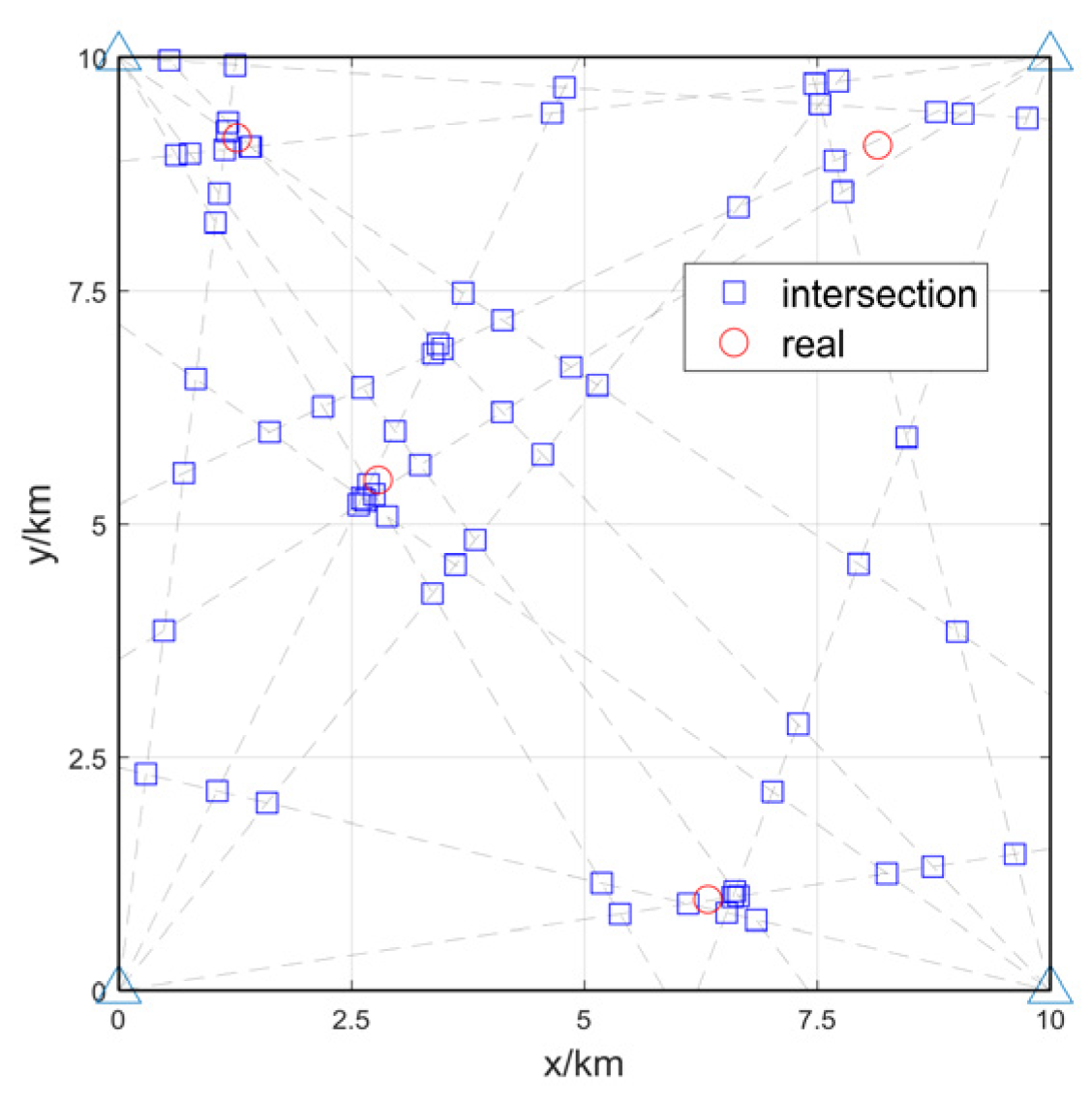
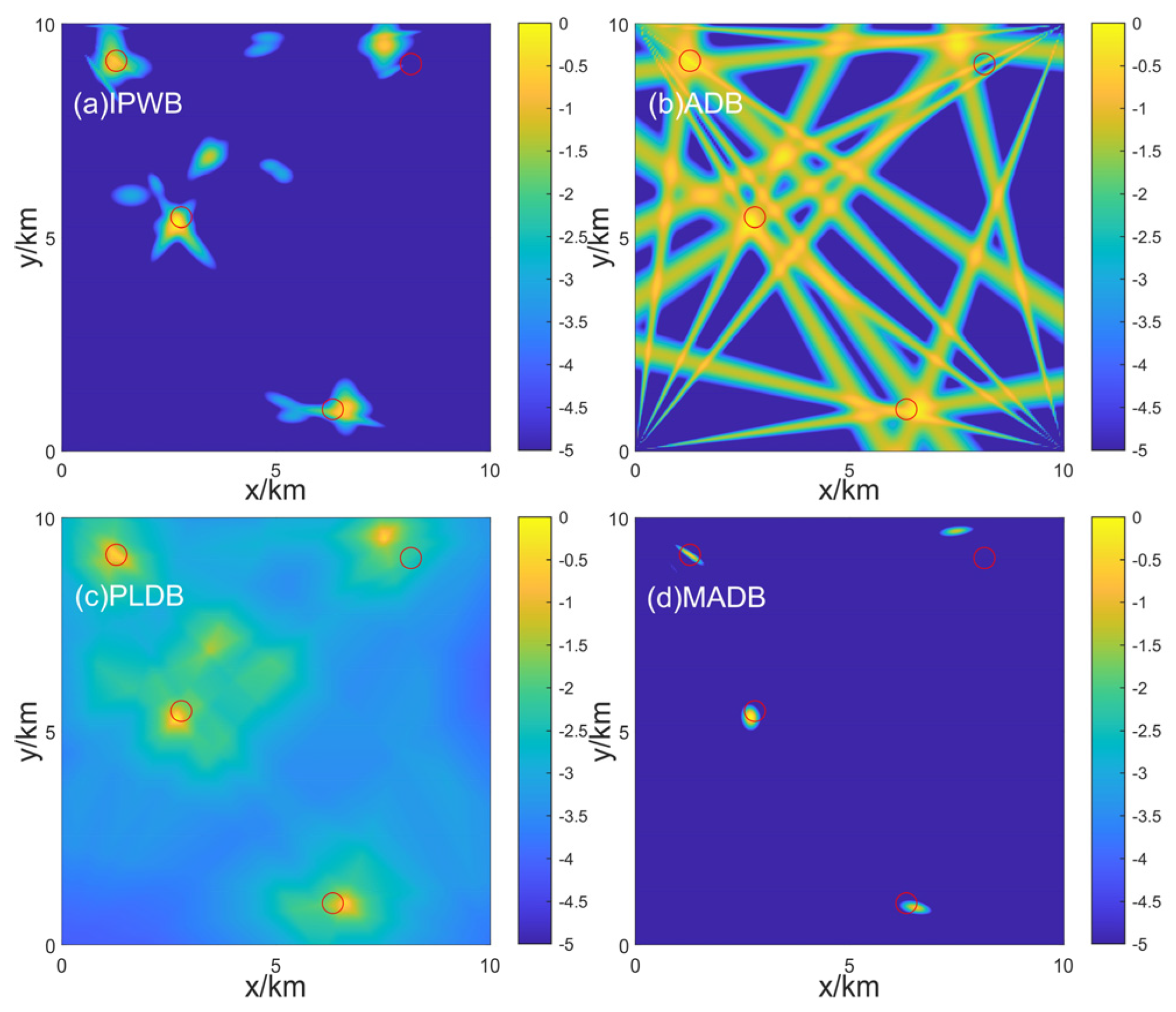
Four random sound sources are set in the observation area, with a bearing angle-difference threshold γ 1 = 20 ° and a predefined bearing-error standard deviation of 1°. Figure 6 shows the distribution of the targets and intersection points. The four hollow triangles represent the receiving arrays, the blue hollow squares represent the retained intersection points, and the red hollow circles indicate the true target locations. The arrays and targets are numbered starting from the south-west corner as target 1, proceeding clockwise, with the observation errors for each array and target shown in Table 1. Figure 7 shows the corresponding spatial likelihood map results for each method. The numerical values of each map are normalized, and, for better comparison, logarithmic results are used. From the figure, it can be observed that peaks appear near the true target locations in the spatial likelihood maps. However, each method also shows relatively significant spurious peaks, meaning that peaks also appear in areas where there are no targets. Therefore, directly extracting targets from the maps could lead to a high likelihood of detecting false targets. Additionally, in the north-east area of the map, the peak for target 3 shows a certain deviation from the true location. By observing the bearing errors from the arrays, it is clear that three of the arrays have larger errors, which causes the peak in the spatial likelihood map to deviate from the true target location.
To validate the localization performance of the multi-target spatial likelihood map after cyclic peak extraction, multiple Monte Carlo simulation experiments are conducted under different conditions. The number of targets is set to range 2 ~ 4 , randomly distributed within the observation area, with the bearing measurement-error standard deviation with the range 1 ° ~ 6 ° , at intervals of 0.5 ° . The Optimal Subpattern Assignment (OSPA) distance [33] is used as the evaluation metric. This method calculates the distance between the true multi-target positions (denoted by the set X = { x 1 , x 2 , x m } , where each element represents the true target position) and the estimated multi-target positions (denoted by the set Y = { y 1 , y 2 , y n } , where each element represents the estimated target position). When m n , the OSPA distance is calculated as follows:
d ¯ p c X , Y = 1 n min π Π n i = 1 m d c x i , y π i p + c p n m 1 p ,
when m > n , d ¯ p c X , Y = d ¯ p c ( Y , X ) . Where d c x , y = min c , d e x , y , and d e is the Euclidean distance between two positions, Π n denotes all permutations of the set 1,2 , , n . The physical interpretation of the OSPA metric is that if the estimation error between the estimated and true values is within a distance penalty parameter c , the p -norm of their difference is calculated. If a true target has no estimate or a false alarm occurs, the distance error c is added once for each missing or false target. Finally, the norm of the cumulative error is averaged. OSPA is widely applied in multi-target localization and tracking [34,35]. In this simulation, the parameters used are c = 700 , p = 2 .
Figure 8 shows the relationship between the average OSPA distance and bearing measurement error, as well as the number of targets, after 2000 Monte Carlo simulations for different methods. From the figure, it can be observed that under the same parameter conditions, the OSPA distance of MADB is consistently lower than that of the other three methods. It is also evident that as the bearing measurement error increases, the OSPA distance tends to approach the value of 700, which is the chosen parameter c . This indicates that when the bearing error becomes large, the positioning accuracy of the results becomes unreliable. The subsequent simulation results for OSPA follow a similar trend.
To verify the improvement in localization performance achieved by the statistical dual-threshold-based cyclic peak extraction method, a comparison is conducted with the direct extraction method from the spatial likelihood map. Figure 9 shows the direct extraction result of the MADB spatial likelihood map with four targets. It can be seen that two false peaks were extracted, indicating that the direct extraction method, when false peaks appear in the spatial likelihood map, may result in the extraction of incorrect peaks, leading to a decrease in localization performance. The bearing errors of each array are shown in Table 2, with the corresponding positions matching those in Table 1. Under the same conditions, the process of multiple extractions using the statistical dual-threshold method is shown in Figure 10. By comparing Figure 9 and Figure 10, it can be observed that multiple extractions can eliminate false peaks, thereby improving the localization performance.
Position nonlinear-least-square (PNLS) [36] is an extension of the single-target NLS method to the multi-target case. The sequential approach (SA) [15] can be used for multi-target localization. The principle is to calculate all possible target positions based on angle combinations using formula (9), and then sum the angle differences between the possible position and the array’s observed angles. The combination with the smallest sum is selected, and the target estimated position is the one corresponding to this optimal combination. The proposed MADB method is compared with PNLS, both before and after cyclic peak extraction. Multiple Monte Carlo simulations were conducted under the same conditions, with the number of targets set to 2 ~ 4 , randomly distributed in the observation area, and the standard deviation of the bearing error set from 1 ° ~ 6 ° with an interval of 0.5 ° . Figure 11 shows the OSPA results for three methods. DMADB (Direct MADB) represents the method of direct extraction from the spatial likelihood map. From the figure, it can be seen that direct extraction results in higher errors, while the error decreases after applying cyclic peak extraction. Furthermore, compared to PNLS, the proposed method achieves lower localization errors, demonstrating better localization performance.
The previous simulations were conducted under ideal conditions, but in real underwater environments achieving a high detection rate is difficult, and interference may exist. Moreover, the original PNLS method does not provide a computation model for cases with missed detections. To compare the proposed method with PNLS under non-ideal conditions, the PNLS method is modified to be applicable even in cases of missed detections. As mentioned in the previous section, the Sequential Approach (SA) method works by taking a bearing result from each array, combining them, and calculating the cost of each combination. The combination with the minimum cost is selected, and this process is repeated until the final positioning result is obtained. However, in the case of missed detections, some arrays may fail to detect certain targets, and the SA method cannot provide an accurate combination for these targets. To address this, we propose a modification to consider all combinations involving three or more arrays. These results are then subjected to a cyclic combination extraction process. Figure 12 illustrates the target extraction process using the MADB method and compares it with the final positioning results of the PNLS method. From Figure 12f, it can be seen that PNLS produces a significant number of false targets. Each array’s observation data include interference at certain azimuth positions from Figure 12f, and Arrays S2 and S4 are missing measurements for certain targets.
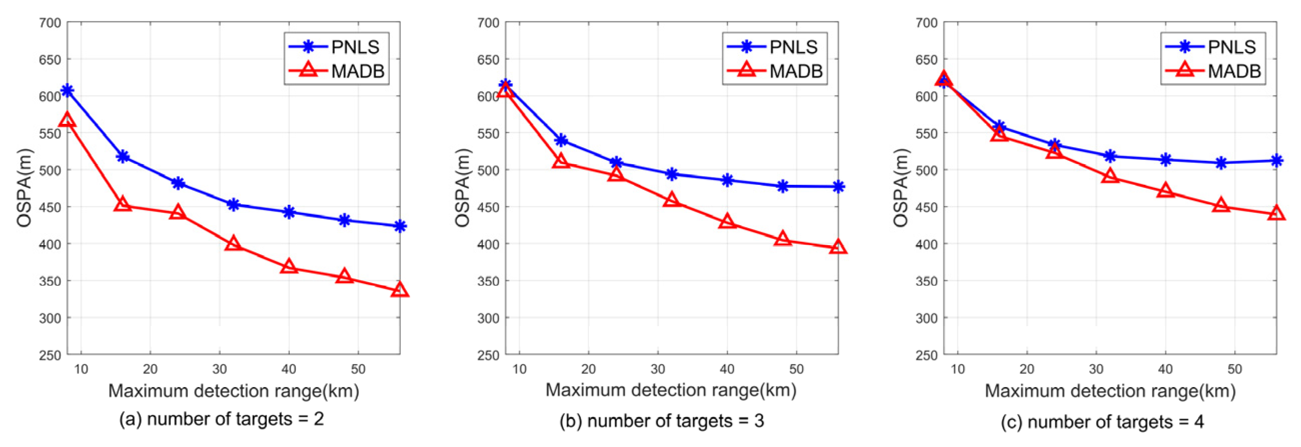
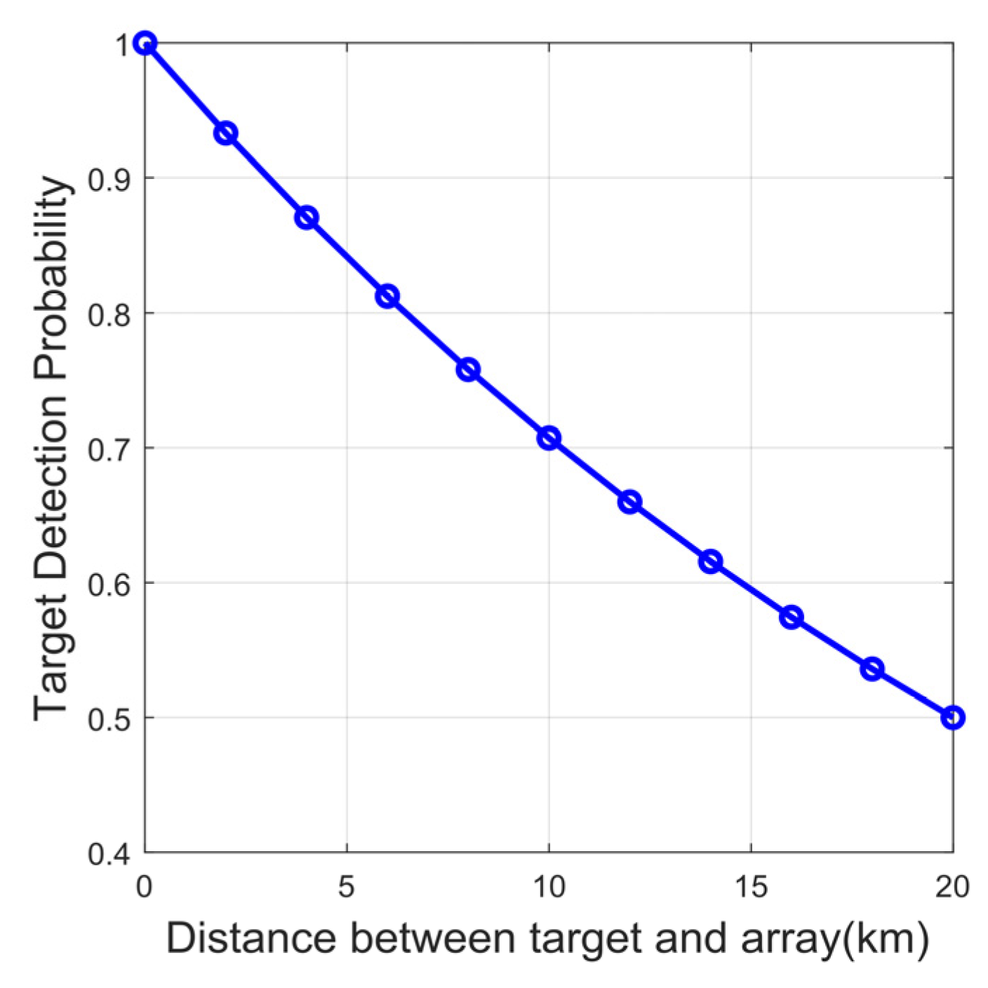
The detection rate for each array is defined in the last section of the first part. During each simulation, a uniform random number is generated between [0, 1], and if the number is smaller than the detection rate, the array fails to detect the target. The detection rate is reflected through multiple simulations. Assuming that all arrays have the same maximum detection range, and the bearing-error standard deviation is set to 2 ° , multiple Monte Carlo experiments are conducted. Figure 13 compares the OSPA results for the two methods under different maximum detection ranges and target numbers. From the figure, it is evident that when the maximum detection range exceeds 15 km, MADB exhibits lower positioning errors, and the positioning errors are reduced by an average of 14.89%, 10.21%, and 7.36%, respectively, when the target number is 2, 3, and 4. When the maximum detection range is below 15 km, the detection rates for targets decrease significantly, resulting in higher errors for both methods. For the case where the maximum detection range of the fixed array is 20 km (i.e., the detection rate for a target at 20 km is 0.5), the detection rate for targets at other distances is given by Equation (13). Figure 14 shows the detection rates for targets at different distances, while Figure 15 presents the comparison of OSPA results for the two methods under different bearing-error standard deviations. From Figure 15, it can be seen that MADB has a lower positioning error compared to PNLS, especially when the bearing error is large, and the positioning errors are reduced by an average of 8.3%, 4.7%, and 3.43%, respectively, when the target number is 2, 3, and 4.
To validate the positioning performance in the presence of interference, directional interference is added to the bearing information from each array. The number of interferences is generated randomly based on an expected number, and the corresponding number of false bearing data is added to the measurements of each array. The false bearing information follows a uniform distribution within the observational bearing of the array. In this scenario, a comparison of the two methods is made under varying expected interference numbers. The bearing-error standard deviation is set to 2°, the maximum detection range of each array is set to 20 km, and the number of targets is set to 2 to 4. The expected number of interferences u ranges from 1 to 10, and the results are averaged over multiple Monte Carlo simulations. Figure 16 presents a comparison of the OSPA results of the MADB and PNLS methods under different numbers of targets and expected interference. From the figure, it can be observed that under conditions with interference, MADB consistently shows lower positioning errors compared to the PNLS method, and the positioning errors are reduced by an average of 5.57%, 3.84%, and 3.02%, respectively, when the target number is 2, 3, and 4.

5. Conclusions and Discussion

This paper proposes several methods for constructing spatial likelihood maps for multi-array bearing-only localization. These methods use only the bearing information from each array to describe the target distribution within the observation area. Additionally, a statistical dual-threshold approach is employed to suppress the extraction of false points. Simulation results show that the spatial likelihood map method based on MADB, after the application of the statistical dual-threshold approach for target extraction, significantly improves localization accuracy. The proposed method demonstrates good localization performance. Moreover, compared to the traditional PNLS method, the proposed method exhibits lower localization errors under conditions where the arrays’ bearings are subject to interference and detection dropout.
The method proposed in this paper sequentially extracts targets from the spatial likelihood map. If the first extracted target is a false target, it will greatly affect the final results. Therefore, when the bearing lines of different targets converge at a single point or are closely spaced, the method may initially extract a false target. In such cases, the localization performance of the method may degrade. In future work, we will consider how to improve the localization performance under these circumstances, such as extracting two or more targets at a time during target extraction using statistical dual-threshold, and considering the optimal solution for simultaneous extraction of multiple targets, which may enhance the localization performance.
In this paper, we primarily conduct a simulation analysis of the proposed method to explore its effectiveness and feasibility under specific conditions. In the future, with the corresponding conditions in place, experimental data will be used for validation. The first step will be to consider whether the parameters of the acoustic-field environment can be incorporated into the proposed method. After establishing the feasibility of the method, simulation and validation will be conducted on experimental data from real-world environments. The experimental data will further validate and refine the proposed method, thereby guiding the direction for subsequent research.
The proposed method holds potential practical applications in multiple-array-bearing-only localization. It could be utilized in various fields such as maritime surveillance. We can use the proposed spatial likelihood map to obtain the target distribution in the monitoring area, which has important reference value for us to accurately locate multiple ships or objects in the ocean.

Author Contributions

Conceptualization, C.H. and B.Z.; validation, C.H., X.Y. and Z.Z.; formal analysis, X.Y. and D.L.; investigation, Z.Z.; resources, X.Y.; data curation, C.H.; writing—original draft preparation, C.H.; writing—review and editing, X.Y. and D.L. All authors have read and agreed to the published version of the manuscript.

Funding

This research was funded by the National Natural Science Foundation of China (Grant No. 12104481).

Institutional Review Board Statement

Not applicable.

Informed Consent Statement

Not applicable.

Data Availability Statement

Data are contained within the article.

Conflicts of Interest

The authors declare no conflicts of interest.

References

  1. Lingren, A.G.; Gong, K.F. Position and Velocity Estimation Via Bearing Observations. IEEE Trans. Aerosp. Electron. Syst. 1978, AES-14, 564–577. [Google Scholar] [CrossRef]
  2. Kaplan, L.M.; Le, Q. On exploiting propagation delays for passive target localization using bearings-only measurements. J. Frankl. Inst. 2005, 342, 193–211. [Google Scholar] [CrossRef]
  3. Eickstedt, D.P. Bearings-only target localization for unmanned underwater vehicles. J. Acoust. Soc. Am. 2011, 130, 2382. [Google Scholar] [CrossRef]
  4. Klein, D.J.; Venkateswaran, S.; Isaacs, J.T.; Burman, J.; Pham, T.; Hespanha, J.; Madhow, U. Localization with sparse acoustic sensor network using UAVs as information-seeking data mules. ACM Trans. Sens. Netw. (TOSN) 2013, 9, 1–29. [Google Scholar] [CrossRef]
  5. Wang, G.Q.; Zhang, C.H.; Yin, L.; Li, Y.; Zhang, Y.F. Underwater target detection and tracking based on array element domain data from multi-arrays. Acta Acust. 2019, 44, 491–502. [Google Scholar] [CrossRef]
  6. Dong, G.; Cao, Z.; Guo, L.H.; Xu, P.; Yan, C. A modified bearings-only target motion analysis method based on frequency β-warping transform in shallow water. Acta Acust. 2019, 44, 513–522. [Google Scholar] [CrossRef]
  7. Fascista, A. Toward integrated large-scale environmental monitoring using WSN/UAV/Crowdsensing: A review of applica-tions, signal processing, and future perspectives. Sensors 2022, 22, 1824. [Google Scholar] [CrossRef] [PubMed]
  8. Kaplan, L.; Le, Q.; Molnar, N. Maximum likelihood methods for bearings-only target localization. IEEE Int. Conf. Acoust. Speech Signal Process. 2001, 5, 3001–3004. [Google Scholar]
  9. Bishop, A.N.; Anderson, B.D.O.; Fidan, B.; Pathirana, P.N.; Mao, G. Bearing-only localization using geometrically constrained optimization. IEEE Trans. Aerosp. Electron. Syst. 2009, 45, 308–320. [Google Scholar] [CrossRef]
  10. Stansfield, R.G. Statistical theory of DF fixing. J. Inst. Electr. Eng.-Part IIIA Radiocommun. 1947, 94, 762–770. [Google Scholar]
  11. Doğançay, K. Bearings-only target localization using total least squares. Signal Process. 2005, 85, 1695–1710. [Google Scholar] [CrossRef]
  12. Doğançay, K. Passive emitter localization using weighted instrumental variables. Signal Process. 2004, 84, 487–497. [Google Scholar] [CrossRef]
  13. Ho, K.C.; Chan, Y.T. An asymptotically unbiased estimator for bearings-only and Doppler-bearing target motion analysis. IEEE Trans. Signal Process. 2006, 54, 809–822. [Google Scholar] [CrossRef]
  14. Griffin, A.; Mouchtaris, A. Localizing multiple audio sources from DOA estimates in a wireless acoustic sensor network. In Proceedings of the IEEE Workshop on Applications of Signal Processing to Audio and Acoustics, New Paltz, NY, USA, 20–23 October 2013. [Google Scholar]
  15. Griffin, A.; Alexandridis, A.; Pavlidi, D.; Mastorakis, Y.; Mouchtaris, A. Localizing multiple audio sources in a wireless acoustic sensor network. Signal Process. 2015, 107, 54–67. [Google Scholar] [CrossRef]
  16. Bishop, A.N.; Pathirana, P.N. Localization of emitters via the intersection of bearing lines: A ghost elimination approach. IEEE Trans. Veh. Technol. 2007, 56, 3106–3110. [Google Scholar] [CrossRef]
  17. Bishop, A.N.; Pathirana, P.N. A discussion on passive location discovery in emitter networks using angle-only measurements. In Proceedings of the 2006 International Conference on Wireless Communications and Mobile Computing, Vancouver, BC, Canada, 3–6 July 2006; pp. 1337–1344. [Google Scholar]
  18. Reed, J.D.; da Silva CR, C.M.; Buehrer, R.M. Multiple-source localization using line-of-bearing measurements: Approaches to the data association problem. In Proceedings of the MILCOM 2008-2008 IEEE Military Communications Conference, San Diego, CA, USA, 16–19 November 2008; pp. 1–7. [Google Scholar]
  19. Omologo, M.; Svaizer, P. Acoustic event localization using a crosspower-spectrum phase based technique. In Proceedings of the ICASSP’94, IEEE International Conference on Acoustics, Speech and Signal Processing, Adelaide, Australia, 19–22 April 1994; Volume 2, pp. II/273–II/276. [Google Scholar]
  20. Brutti, A.; Omologo, M.; Svaizer, P. Speaker localization based on oriented global coherence field. In Proceedings of the Ninth International Conference on Spoken Language Processing, Pittsburgh, PA, USA, 17–21 September 2006. [Google Scholar]
  21. Huang, Y.; Tong, J.; Hu, X.; Bao, M. A Robust steered response power localization method for wireless acoustic sensor networks in an outdoor environment. Sensors 2021, 21, 1591. [Google Scholar] [CrossRef]
  22. Do, H.; Silverman, H.F. A fast microphone array SRP-PHAT source location implementation using coarse-to-fine region con-traction (CFRC). In Proceedings of the IEEE Workshop on Applications of Signal Processing to Audio and Acoustics, New Paltz, NY, USA, 21–24 October 2007; pp. 295–298. [Google Scholar]
  23. Cobos, M.; Marti, A.; Lopez, J.J. A modified SRP-PHAT functional for robust real-time sound source localization with scalable spatial sampling. IEEE Signal Process. Lett. 2010, 18, 71–74. [Google Scholar] [CrossRef]
  24. Aarabi, P. The fusion of distributed microphone arrays for sound localization. EURASIP J. Adv. Signal Process. 2003, 2003, 860465. [Google Scholar] [CrossRef]
  25. Brutti, A.; Omologo, M.; Svaizer, P. Multiple source localization based on acoustic map de-emphasis. EURASIP J. Audio Speech Music Process. 2010, 2010, 1–17. [Google Scholar] [CrossRef]
  26. Pattipati, K.; Deb, S.; Bar-Shalom, Y.; Washburn, R. A new relaxation algorithm and passive sensor data association. IEEE Trans. Autom. Control 1992, 37, 198–213. [Google Scholar] [CrossRef]
  27. Deb, S.; Pattipati, K.; Bar-Shalom, Y.; Yeddanapudi, M. A generalized s-dimensional algorithm for multisensor multitarget state-estimation. In Proceedings of the 1994 33rd IEEE Conference on Decision and Control, Lake Buena Vista, FL, USA, 14–16 December 1994; Volume 4, pp. 3293–3298. [Google Scholar]
  28. Liu, B.; Towsley, D. A study of the coverage of large-scale sensor networks. In Proceedings of the 2004 IEEE International Conference on Mobile Ad-Hoc and Sensor Systems (IEEE Cat. No. 04EX975), Fort Lauderdale, FL, USA, 25–27 October 2004; pp. 475–483. [Google Scholar]
  29. Wang, G.Q.; Zhang, C.H.; Yin, L.; Li, Y.; Zhang, Y.F. Underwater multi-target tracking using improved multi-sensor multi-Bernoulli filter. Acta Acust. 2021, 46, 508–518. [Google Scholar] [CrossRef]
  30. Yu, J.; Wang, Y.L. Data Association Algorithm for Bearing-Crossing Localization of Multiple Passive Sonars. Command. Infor-Mation Syst. Technol. 2018, 9, 65–69. [Google Scholar]
  31. Xin, G.; You, H.; Xiao, Y. Gray track-to-track correlation algorithm for distributed multitarget tracking system. Signal Process. 2006, 86, 3448–3455. [Google Scholar] [CrossRef]
  32. Yu, X.; Chen, X.; Huang, Y.; Zhang, L.; Guan, J.; He, Y. Radar moving target detection in clutter background via adaptive dual-threshold sparse fourier transform. IEEE Access 2019, 7, 58200–58211. [Google Scholar] [CrossRef]
  33. Schuhmacher, D.; Vo, B.T.; Vo, B.N. A consistent metric for performance evaluation of multi-object filters. IEEE Trans. Signal Process. 2008, 56, 3447–3457. [Google Scholar] [CrossRef]
  34. Yan, J.; Jiao, H.; Pu, W.; Shi, C.; Dai, J.; Liu, H. Radar sensor network resource allocation for fused target tracking: A brief review. Inf. Fusion 2022, 86, 104–115. [Google Scholar] [CrossRef]
  35. Khaleghi, B.; Khamis, A.; Karray, F.O.; Razavi, S.N. Multisensor data fusion: A review of the state-of-the-art. Inf. Fusion 2013, 14, 28–44. [Google Scholar] [CrossRef]
  36. Kaplan, L.M.; Molnar, P.; Le, Q. Bearings-only target localization for an acoustical unattended ground sensor network. Unattended Ground Sensor Technolo-gies and Applications III. Spie 2001, 4393, 40–51. [Google Scholar]
Figure 1. The schematic of the sensor network node distribution is shown in the figure. The black dashed lines represent the bearing lines from each node, assuming no observation errors. The green solid circles indicate the true target positions within the observation area. The blue solid circles represent the array positions.
Jmse 13 00109 g001
Figure 2. Multi-target data-association-problem diagram. The red circles represent the true positions of the targets. The blue solid circles represent the node positions and the dashed lines represent the bearing results from the four nodes. The solid squares represent the intersection points.
Jmse 13 00109 g002
Figure 3. Three-node intersection diagram. The letter S represents the node positions. The letter P and Q represent the intersection points. The letter l represents the bearing lines.
Jmse 13 00109 g003
Figure 4. The bearing crossing diagram and the spatial likelihood maps for each method are shown. (a) illustrates the distribution of the target and intersection points, with the red circles in each diagram representing the true target location. (bf) show the spatial likelihood maps for different methods. The coordinate scale for each of these figures is the same as that in Figure 4a, and the triangles represent the node positions.
Jmse 13 00109 g004
Figure 5. The comparison of the RMSE for each method under single-target conditions: (a) for a random target, and (b) for a fixed target [ 8321,6099 ] T .
Jmse 13 00109 g005
Figure 6. The scenario of multi-target-bearing intersections and target distribution. The triangles represent the node positions.
Jmse 13 00109 g006
Figure 7. The illustrations of various multi-target spatial likelihood maps are shown. In each diagram, the red hollow circles represent the true target positions. (ad) display the multi-target spatial likelihood maps for different methods.
Jmse 13 00109 g007
Figure 8. The comparison of OSPA distances for each method is shown in (ac), where each figure represents a different number of targets.
Jmse 13 00109 g008
Figure 9. The schematic diagram of direct extraction localization results, where the red hollow circles represent the true positions of the targets, and the white squares represent the results of directly extracting the four highest peaks from the map.
Jmse 13 00109 g009
Figure 10. The target extraction-process diagram based on statistical dual threshold method, where the red hollow circles represent the true target positions, and the white hollow squares represent the target extraction results.
Jmse 13 00109 g010
Figure 11. Comparison of OSPA results between MADB and PNLS methods under different numbers of targets and different bearing-error conditions.
Jmse 13 00109 g011
Figure 12. The target extraction process and results comparison are as follows. (ae) show the extraction process using the MADB method. The red hollow circles represent the true target positions, and the white hollow squares represent the extracted target results. (f) compares the localization results of MADB and PNLS.
Jmse 13 00109 g012aJmse 13 00109 g012b
Figure 13. Comparison of OSPA distance results between the MADB and PNLS methods under different maximum detection ranges and target numbers.
Jmse 13 00109 g013
Figure 14. The detection probability of the array for targets at different distances when the maximum detection range is 20 km.
Jmse 13 00109 g014
Figure 15. Comparison of OSPA results between the MADB and PNLS methods under different bearing-error standard deviations.
Jmse 13 00109 g015
Figure 16. Comparison of OSPA results between the MADB and PNLS methods under different expected interference numbers when the maximum detection range is 20 km.
Jmse 13 00109 g016
Table 1. The observation errors (°) of each array for each target are as follows.
Target 1 (Southwest)Target 2 (Northwest)Target 3 (Northeast)Target 4 (Southeast)
Node 1 (southwest)0.70.73.60.1
Node 2 (northwest)1.20.12.81.5
Node 3 (northeast)0.70.71.31.4
Node 4 (southeast)1.60.23.01.4
Table 2. The observation errors (°) of each array for each target are as follows.
Target 1 (Southwest)Target 2 (Northwest)Target 3 (Northeast)Target 4 (Southeast)
Node 1 (southwest)0.70.92.51.7
Node 2 (northwest)1.10.31.32.7
Node 3 (northeast)2.10.40.10.9
Node 4 (southeast)2.21.00.41.7
Disclaimer/Publisher’s Note: The statements, opinions and data contained in all publications are solely those of the individual author(s) and contributor(s) and not of MDPI and/or the editor(s). MDPI and/or the editor(s) disclaim responsibility for any injury to people or property resulting from any ideas, methods, instructions or products referred to in the content.