Real Time Vessel Detection Model Using Deep Learning Algorithms for Controlling a Barrier System

Abstract

This study addresses marine pollution caused by debris entering the ocean through rivers. A physical and bubble barrier system has been developed to collect debris, but an effective identification and classification system for incoming vessels is needed. This study evaluates the effectiveness of deep learning models in identifying and classifying vessels in real time. The YOLO (You Only Look Once) v5 and v8 models are evaluated for vessel detection and classification. A dataset of 624 images representing 13 different types of vessels was created to train the models. The YOLOv8, featuring a new backbone network, outperformed the YOLOv5 model, achieving a high mean average precision (mAP@50) of 98.9% and an F1 score of 91.6%. However, YOLOv8’s GPU consumption increased by 116% compared to YOLOv5. The advantage of the proposed method is evident in the precision–confidence curve (PCC), where the accuracy peaks at 1.00 and 0.937 confidence, and in the achieved frames per second (fps) value of 84.7. These findings have significant implications for the development and deployment of real-time marine pollution control technologies. This study demonstrates that YOLOv8, with its advanced backbone network, significantly improves vessel detection and classification performance over YOLOv5, albeit with higher GPU consumption. The high accuracy and efficiency of YOLOv8 make it a promising candidate for integration into marine pollution control systems, enabling real-time identification and monitoring of vessels. This advancement is crucial for enhancing the effectiveness of debris collection systems and mitigating marine pollution, highlighting the potential for deep learning models to contribute to environmental preservation efforts.

1. Introduction

This work is part of the REPERA project, led by CT Engineers, to eliminate waste in marine and fluvial environments. Rivers are a major source of debris entering the ocean, which is of concern for the global maritime industry. It is possible to significantly reduce the number of debris that is deposited in the ocean environment by utilizing debris pollution collecting systems; one such system is a one-of-a-kind combination of a physical barrier and a bubble barrier (see Figure 1). These collecting systems do not use any ship detection methods and do not consider the interaction of anti-pollution methods and ships sailing in their surroundings. It is important to detect these ships to avoid collisions or the dragging of those collecting systems. As a result of this gap, this research is conducted to evaluate the performance of two deep learning models (YOLO v5 and v8) and select the best option to identify any ship coming to the barrier and, after ship identification, to activate the movement of the physical system, in this case, a floating barrier. Having a deep learning (DL)-controlled physical and bubble barrier system that is operational 24/7 makes its deployment possible in any environment, regardless of maritime traffic in the area to be protected. Therefore, we propose to analyze two DL algorithms (YOLO v5 and v8) that can accurately detect all kinds of vessels in real time. The processed images are also used to detect the ship’s approach speed. This is an important factor in determining when it is necessary to lower the physical barrier and generate the bubble barrier in its place. Knowing the time necessary to perform these two tasks and determining the speed of the vessel is crucial to knowing if there is enough time to perform them. Although the speed reached by ships is not high in the areas (estuaries, canals, and lakes) where the installation of this type of barrier is planned, their speed is a fact to be considered for the optimized operation of the system. It is not possible to accurately determine the speed of an object solely based on the size of the bounding box provided by YOLO. The bounding box size alone does not provide enough information to calculate the speed of the vessel. Therefore, we determine the speed at which a ship approaches using camera images, which involves a combination of computer vision and motion analysis techniques. The general approach is as follows:

• Camera Calibration: We need to calibrate the camera to obtain the intrinsic parameters (focal length and principal point) and distortion coefficients. This step is crucial for accurate measurements in real-world units.
• Object Detection: This is the focus of this paper. We detect and track the ship in each frame. The model provides us with bounding box coordinates for the ship.
• Distance Measurement: We determine the real-world distance between the camera and a reference point on the ship. This information comes from a lidar sensor.
• Speed Calculation: We calculate the speed of the ship using the change in position of the ship over time. The speed (v) can be calculated using the formula $v={\displaystyle \frac{∆d}{∆t}}$, where Δd is the change in distance, and Δt is the change in time between consecutive frames.
• Frame Rate: We consider the frame rate of the camera (f_frame) when calculating the time difference between frames. The time difference (Δt) can be calculated as $∆t={\displaystyle \frac{1}{f_{frame}}}$.

Because the objective of this type of containment barrier is not to be in the open sea but in inland navigation areas such as rivers, lakes, or canals, it does not seem necessary to incorporate an algorithm to smooth velocity. This is an algorithm to stabilize the velocity estimation, especially if the ship’s motion is not constant. The most likely thing in these cases is that the speed of the vessel will be low and the movements smooth. Additionally, environmental factors, such as tidal currents, wind, or waves, do not affect ship motion in those kinds of locations.

It is important to note that the accuracy of speed estimation depends on the quality of the object detection, camera calibration, and distance measurements. Additionally, using multiple sensors or integrating information from other sources (such as an AIS—automatic identification system) can enhance the accuracy of the speed estimation in a maritime context. In fact, AIS ship tracking can be used to validate and calibrate speed estimation.

Finally, we propose a system implementation with a combination of cameras and lidar sensors to provide additional information about the distance between the vessel and the barrier. The training of both YOLO algorithms included the classification of ships by type to know the object’s actual size, so we can use the bounding box coordinates to determine the speed of the ship, with the additional information of distance and time.

However, object detection models like YOLO are primarily designed to locate objects in images or frames and provide bounding box coordinates and object classifications, but they do not directly measure speed. Speed estimation typically requires additional data and calculations beyond what an object detection model can provide. In this work, we enhanced the vessel detection with speed data to achieve the autonomous movement of the barrier system. The analysis of this additional information is part of the development of a Python application capable of managing the vessel data, the acquisition data, and the YOLO results.

2. Literature Review

Machine learning algorithms for object detection, which have been developed in recent years, are being applied to the detection of pollution and other elements. This results in the efficiency of anti-pollution barriers, or any other device used to contain contamination. In the sea, one of the biggest sources of pollution is due to oil residues. Monitoring these oil slicks is important to prevent them from reaching protected ecosystems. In [1], a YOLO v4 algorithm is used for tracking sunken and submerged oil spills. They used image data from real oil pollution moving under breaking waves. Ref. [2] monitored sandy beach ecosystems to ensure their conservation. A YOLO algorithm using video images was applied to detect active bulldozers and identify anthropogenic changes in the coast.

In the development of the REPERA project, the use of this type of algorithm is proposed not only for the detection of garbage in fluvial areas or near ports but also for the detection of ships. The identification of the possible ships that are going to cross the area of the containment barrier will allow its automatic movement to let the ship pass. Some authors have already proposed different approaches to ship detection for avoiding ship–bridge collisions through machine learning algorithms, such as in Ref. [3]. In Ref. [4], a convolutional neural network (CNN) was proposed for ship detection through infrared images. In both cases, images oriented toward the profile of the ship were used, but some works used aerial ship images for detecting them, such as in [5,6], where faster region-based convolutional neural networks (FRCNs) were used to detect multi-class objects in remote sensing images. The datasets used include the aircraft dataset, Aerial-Vehicle dataset, and SAR-Ship dataset [7]. SAR (synthetic-aperture radar) images were used in [8], where a convolutional neural network (CNN) was applied within a transfer learning framework consisting of a knowledge transfer network and a ship detection network to address the data acquisition and labeling problem for ship detection. In [9], the authors used open datasets of ship images (TerraSAR-X) and these initial conditions; they argued that CNN algorithms achieve ship detection but with many missed and false results, so they presented a modified YOLO v5 model with a mean average precision of 95.02. However, the initial conditions and contexts of their study do not align with those of our approach. The work developed in [9], as well as the work in [10], are used as references for the limitations of YOLOv5. However, in this case, the authors were aware that most existing algorithms only focus on target recognition performance and ignore the model’s size and computational efficiency. Therefore, they proposed a YOLOv5-n lightweight model as the baseline algorithm. The experimental results show that the model can achieve an F1 score performance of 61.26 and an FPS performance of 68.02.

In autonomous ships, the detection of other ships is essential to avoid possible collisions. Therefore, the application of these types of algorithms is essential for ship safety navigation, especially when it comes to small ships. A mask regional convolutional neural network (Mask-CNN) technique was presented in [10,11] to detect small ships through real-world samples. Additionally, CNN can be used to enhance ship performance by using data flow charts recorded for the ship’s engine Ref [11].

All these works use different approaches of CNN or YOLO versions. There are differences and similarities between YOLO and CNN, as well as between different versions of YOLO [12]. The research conducted in Ref. [13] offered an in-depth analysis of CNN and identified two variables that contributed to the success and evolution of the model. The research focused on CNN models as one of the most prominent deep learning models. The authors proposed the use of stacked layers to create a larger network and implement more complex network topologies. They further presented a technique to optimize the number of blocks and layers, as well as the hyperparameters in the CNN architecture, with the aim of finding and optimizing a CNN model at a low computational cost. Several other studies have employed the robustness of CNN to solve various computer vision problems. Ref. [14] applied CNN in face detection, while Ref. [15] focused on pedestrian detection. Ref. [16] implemented CNN for pose detection, Ref. [17] for content-based image retrieval, and Ref. [18] for video analysis.

However, despite these advances, some challenges still exist, such as inaccurate localization. Ref. [19] addressed this issue by backing up the high-capacity CNN structure with a Bayesian optimization search algorithm that proposes more precise bounding boxes for detected objects. They also employed a structured loss technique to train the CNN model, which penalizes inaccurate localizations. Ref. [20] proposed a novel geocentric embedding for images to deal with the problem of object detection for RGB-D images. The approach encoded the height above ground and the angle with gravity for each pixel, in addition to the horizontal disparity, thereby enhancing the accuracy of CNN models.

The development of the faster region-based convolutional network (Faster R-CNN) was a significant improvement on CNN for object detection tasks. The Faster R-CNN model was introduced in Ref. [21] to address the need to improve the efficiency of the CNN architecture for object detection. Faster R-CNN uses a fully convolutional network (FCN) with the ability to predict object bounds and scores simultaneously. It operates on a specific convolutional layer, which is shared with the object detection network. The FCN takes an input image of arbitrary size and generates a set of rectangular object proposals. It slides over the convolutional feature map and connects to an n × n spatial window, where a low-dimensional vector is obtained and fed into two sibling fully connected layers, the box-classification layer (cls) and the box-regression layer (reg).

The Faster R-CNN model can be trained with different deep learning frameworks, including Caffe and TensorFlow. Ref. [21] demonstrated the effectiveness of Faster R-CNN in improving detection accuracy and speed by training the model with Caffe. Ref. [22] further adapted the joint-training scheme of the Faster R-CNN framework from Caffe to TensorFlow, providing a baseline implementation for object detection.

The YOLO algorithm was presented as a new method for object detection in Ref. [23], which applied a regression problem to frame detection to identify bounding boxes and confidence levels. YOLO region proposal-based frameworks usually consist of multiple stages, including region proposal generation, CNN feature extraction, classification, and bounding box regression. These stages are often trained separately, leading to a bottleneck in real-time deployment due to the significant amount of time required to handle the different components. To reduce computation time, a one-step mapping from image to bounding box and classification is required, and YOLO is a pioneering model that implements this approach. The model works by dividing the input image into an S × S grid, and each grid cell is responsible for detecting any object whose center falls within that cell. Each grid cell predicts bounding boxes and confidence scores for those boxes.

Ref. [24] proposed an updated version of the YOLO model, YOLOv2, with the aim of improving both accuracy and speed without scaling the network. After that, this algorithm underwent significant changes with the release of its third version, YOLOv3. Unlike its predecessors, YOLOv3 appends prediction layers to the side of the network, making predictions at three scales in layers 82, 94, and 106. By concatenating shallower layers with deeper layers, YOLOv3 can better preserve fine-grained features and accurately detect objects of varying sizes.

Another major improvement in YOLOv3 is the introduction of the idea that a grid cell can predict multiple objects at the same time. In previous versions, each grid cell was responsible for predicting only one object, but now, multiple objects can be detected even if they are predicted by the same cell. It addressed the issues of detecting small objects with multiple-scale detections and concatenating shallower layers with deeper ones.

Ref. [25] developed a modified version of YOLOv3. YOLOv4’s feature extractor backbone is based on a cross-stage partial network (CSPNet) and uses a new architecture called CSPDarknet53 [26]. The head of YOLOv4 uses a YOLO layer and implements several techniques to improve object detection. The testing of the YOLOv4 model on the MS COCO dataset showed that it achieved a higher accuracy than YOLOv3 [25,27].

One month following the release of YOLOv4, Ultralystics LLC researcher Glenn Jocher and his team unveiled YOLOv5, a new iteration of the YOLO family [28]. YOLOv5 has a similar architecture to YOLOv4. However, YOLOv5 has some engineering advantages over YOLOv4, which stem from its use of Python rather than the C programming language. For instance, Python is a more accessible language for developers, which could make installation and integration of YOLOv5 onto Internet of things (IoT) devices more manageable.

In YOLOv5, the initial input is an image with a resolution of 640 × 640 × 3, which undergoes a slicing operation to become a 320 × 320 × 12 feature map. Subsequently, a convolution operation involving 32 convolution kernels is employed, resulting in a final 320 × 320 × 32 feature map. YOLOv5 also has a bottom-up feature pyramid structure that combines feature aggregation from different layers to detect objects of different sizes. A recent study by [29] compared the performance of YOLOv3, YOLOv4, and YOLOv5 on the MS COCO dataset. The study found that YOLOv5 outperformed YOLOv4 and YOLOv3 in terms of accuracy. However, YOLOv3 had a faster detection speed compared to YOLOv4 and YOLOv5. Interestingly, the detection speeds of YOLOv4 and YOLOv5 were found to be identical.

The latest version of YOLO, known as YOLOv8, is currently available as an online repository but has yet to be published in a research paper. Despite this, it is possible to gain some insights into the model by analyzing the information available in the repository. One of the key differences between YOLOv8 and previous versions is that YOLOv8 is an anchor-free model. This means that instead of predicting the offset from a known anchor box, it directly predicts the center of an object. This approach reduces the number of box predictions, which can speed up the non-maximum suppression (NMS) process, a post-processing step that is used to filter out redundant object detections after the inference.

The state of the art in this kind of algorithm is YOLO-NAS (You Only Look Once—Neural Architecture Search). It refers to a YOLO-based model that incorporates neural architecture search techniques to automatically discover the optimal neural network architecture for object detection [30]. NAS is a technique that searches for the best neural network architecture by evaluating various combinations of layers and structures. Some aspects of YOLO-NAS might include the following:

• Architecture search: YOLO-NAS uses neural architecture search to find the most effective architecture for the task of object detection.
• Efficiency: YOLO-NAS aims to find a network architecture that is both accurate and computationally efficient.

In [31], a novel detection method (ESP-YOLO) was proposed to improve the detection accuracy and efficiency. The algorithm was conducted on embedded platforms in harvesting robots to detect table grapes in complex scenarios, including the overlap of multi-grape adhesion and the occlusion of stems and leaves. The mAP@0.5:0.95 of ESP-YOLO surpasses that of other advanced methods by 3.7–16.8%. Deploying YOLO on resource-constrained edge devices poses challenges due to its substantial memory requirements. In [32], the authors proposed MPQ-YOLO, an ultra-low mixed-precision quantization framework designed for edge device deployment. The core idea was to integrate 1-bit backbone quantization and 4-bit head quantization with dedicated training techniques. Experiments on VOC and COCO datasets demonstrate that MPQ-YOLO achieves a good trade-off between model compression and detection performance.

In summary, YOLOv5 and YOLOv8 are specific iterations of the YOLO series with improvements in architecture and training techniques, while YOLO-NAS is a general concept that refers to using neural architecture search to find an optimal YOLO-based architecture for object detection. So, we decided to focus on YOLOv5 and YOLOv8 to achieve a more practical result for our project.

3. Implementation of YOLOv5 and YOLOv8

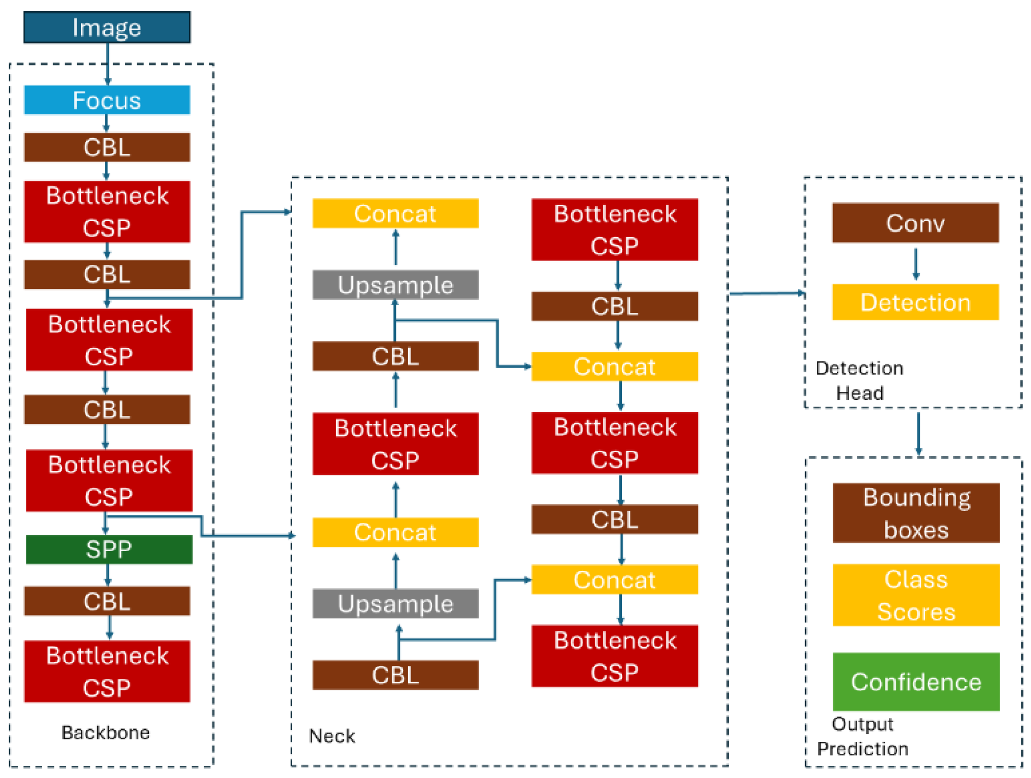
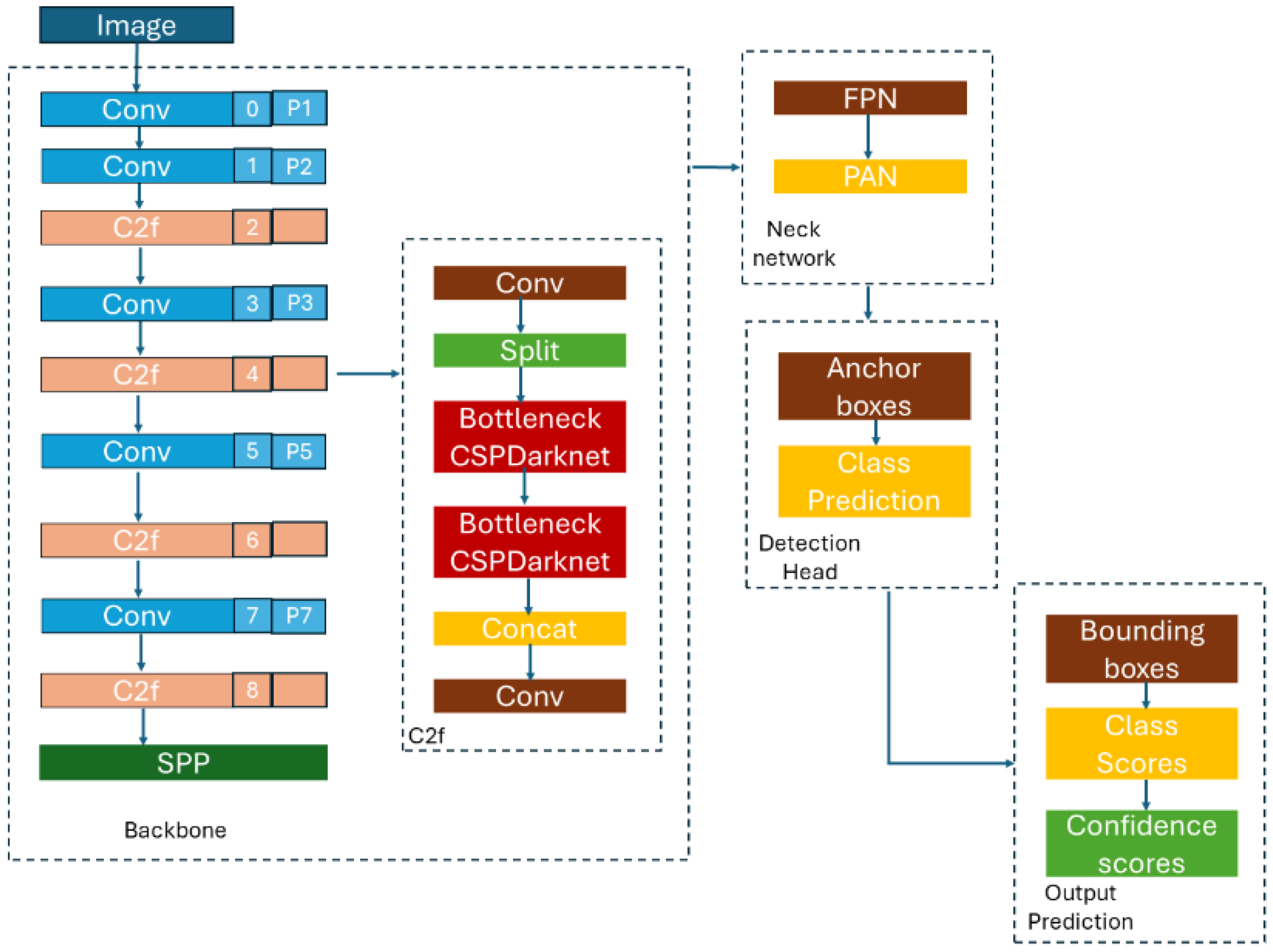
In this work, a supervised learning technique has been implemented and developed using a vessel dataset. The algorithms YOLOv5 (Figure 2) and YOLOv8 (Figure 3) were tested to determine which of them achieves better results in real time. The YOLO architecture has 24 convolutional layers followed by 2 fully connected layers and uses a 1 × 1 reduction layer followed by 3 × 3 convolutional layers. Overall, YOLO is an extremely fast model that achieves a frame rate of 45 frames per second (FPS), producing fewer false positives in the background.

The backbones of YOLOv5 and YOLOv8 have some similarities and differences in their architecture and design. The architecture of YOLOv5 uses the CSP (cross-stage partial) Darknet backbone and includes convolutional layers and SPP (spatial pyramid pooling) blocks. YOLOv8 introduces new improvements over this backbone. YOLOv5 components are convolutional layers as initial layers to process the input image and extract basic features, CSP blocks to split feature maps, and SPP blocks that pool features at multiple scales, capturing context at different levels. YOLOv8 has the same main components but adds new modules with new types of layers aiming for higher accuracy and efficiency. YOLOv5 enhances feature extraction through repeated convolutional and CSP layers, which help in retaining high-level semantic information while reducing spatial resolution. Instead, YOLOv8 is designed to improve upon the feature extraction capabilities of YOLOv5 through deeper networks, better normalization techniques, and more efficient architectural designs. Therefore, the backbones of YOLOv5 and YOLOv8 are designed to efficiently extract features from images, but YOLOv8 likely incorporates more recent advancements in deep learning to enhance both performance and efficiency.

A dataset has been created through the collection of 260 images, consisting of 20 pictures of each of the 13 different vessels, which consists of a passenger ship, rescue vessel, fishing support vessel, general cargo ship, cement carrier, tug vessel, vehicle carrier, oil products tanker, and bulk carrier. After the data gathering for the images was completed, a data-cleaning technique was implemented to ensure that the images were ready for use, consistent, and accurate. This strategy involved the use of visual inspection, which included manually identifying and eliminating defective images, duplicates, or low-resolution images. Subsequently, six data augmentation techniques were implemented. Techniques such as image blurring, shearing, flipping, varying image brightness, and others were applied to augment the dataset to meet the requirements of deep learning, which stipulates that enough images must be included in the dataset for each of the classes.

3.1. Tools and Environment Used

Google Colaboratory Version 3.10, often known as “Colab”, is a product developed by Google Research. The free and premium access to computing infrastructure such as storage, memory, processing capacity, graphics processing units (GPUs), and tensor processing units (TPUs) from Colab was leveraged; hence, there was no need to upgrade the computer hardware to meet Python Version 3.10’s CPU/GPU-intensive workload requirements to use Colab. Additionally, notebook sharing, special library installation, pre-installed libraries (NumPy Version 2.0.1, Pandas Version 2.2.2, Matplotlib Version 3.9.1, PyTorch Version 2.1.0, TensorFlow Version 2.16.1, and Keras Version 2.15.0), extra cloud storage, and GitHub integration are some of the capabilities included with the Colab platform.

To ensure reproducibility and consistency, a set of libraries were utilized within the environments, with their respective versions: urllib3, glob2, Pillow (7.1.2), PyYAML (5.3.1), certify (2022.12.7), opencv-python-headless (4.5.1.48), chardet (4.0.0), numpy (1.18.5), matplotlib, kiwisolver (1.3.1), tqdm (4.41.0), cycler (0.10.0), pyparsing (2.4.7), python-dotenv (0.21.0), requests-toolbelt (0.10.1), roboflow (0.2.25), urllib (3-1.26.6), wget (3.2).

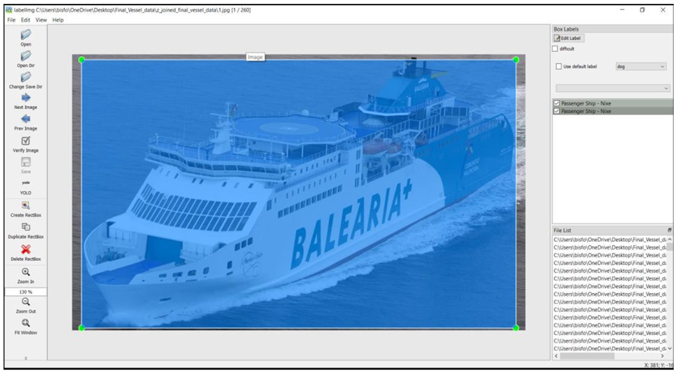
3.2. Dataset Labeling

The data collection contains images that have been manually labeled by using a tool called LabelImg Version 1.4.0. Each image is labeled by defining bounding boxes that fully encircle the desired objects (vessels) in the image and selecting their corresponding classes, as demonstrated in Figure 4. This process was repeated for all images in the dataset.

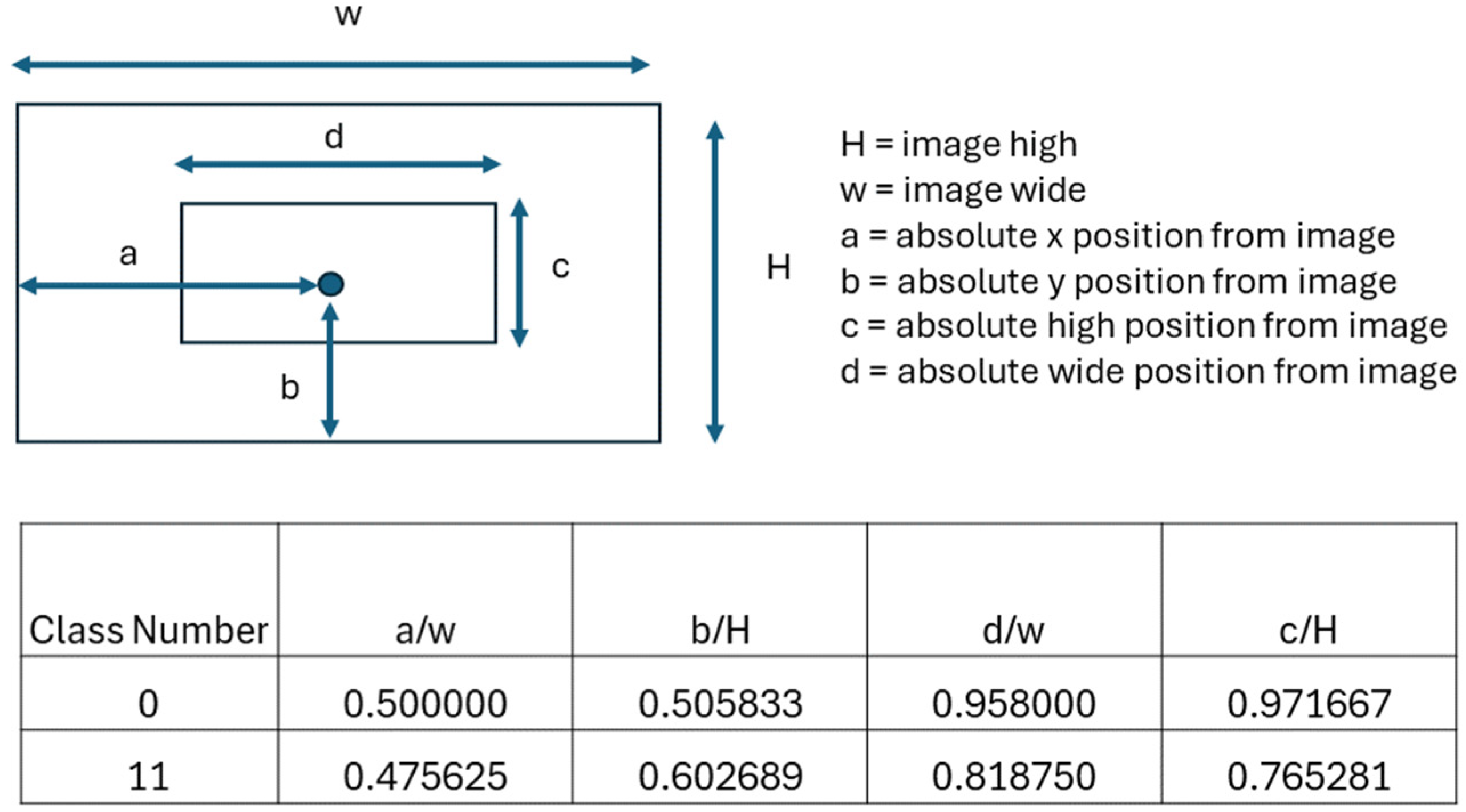
After the labeling process was completed for all the images, a .txt file known as an “Annotation file” was generated for each image (Figure 5). This file contained information about the class attribute of the objects for all the images with the coordinates of the bounding boxes that surrounded the object (vessel).

The labeled images are used to train the model, but it is not necessary to label the images in a real implementation of the system. Using YOLOv8 or YOLOv5 with unlabeled data is challenging but feasible through methods like transfer learning, semi-supervised learning, weak supervision, and synthetic data generation. In this case, we apply data augmentation techniques to enhance the robustness of the model trained on limited labeled data. Therefore, there is no need for manual labeling in a real-time implementation.

3.3. Data Training, Validation, and Testing Split

A training, testing, and validation split was created to ensure that the model is effectively generalizing, as opposed to simply learning the training data by memory. A training set consisting of 85% of the data, a validation set consisting of 8% of the data, and a testing set consisting of 4% of the data was generated from the raw image data that was collected (Figure 6).

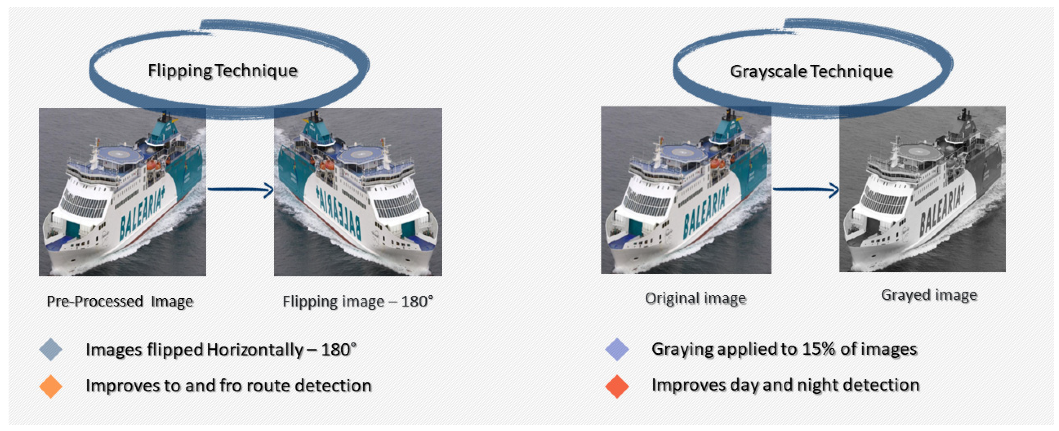
Several data augmentation methods [1] have been used to improve the generalizability of the model’s performance, and this was accomplished by increasing the diversity of learning examples for the model. For the dataset, the methods applied are as follows:

• Flip—horizontal (Figure 7);
• Grayscale—applied to 15% of images (Figure 7).
• Blur—up to 1.25 px (Figure 8);
• Noise—up to 3% pixels (Figure 8);
• Shear—±10° horizontal, ±10° vertical (Figure 9);
• Brightness—between −25% and +25% (Figure 9);

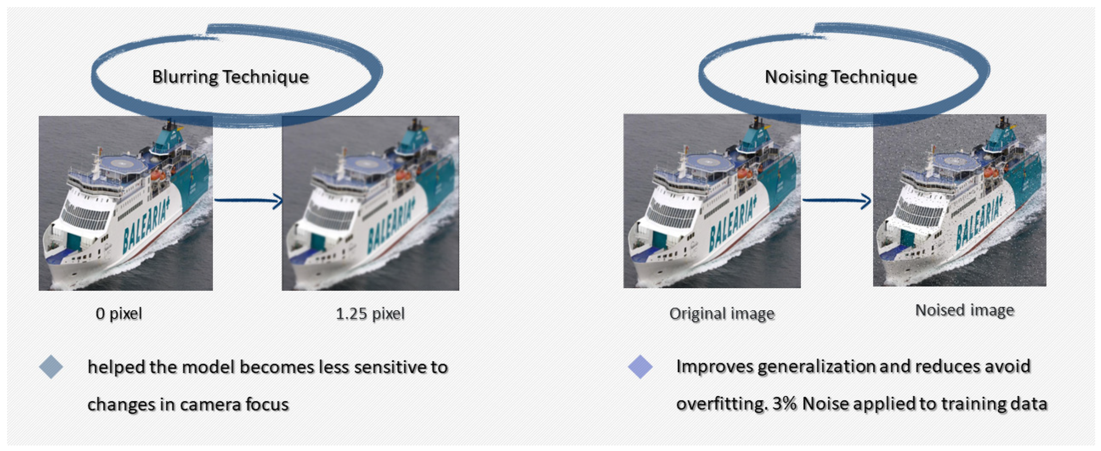
To improve the performance of the model by making it less sensitive to the orientation of the subject, it was flipped around the x-axis, along with the annotations it contained. Using shearing also brought variety to the dataset in terms of viewpoint and made the model more resistant to changes in camera and subject pitch and yaw. For the model to function well in a variety of lighting conditions, it is considered important that the image brightness is also varied. This makes the model more resistant to changes in lighting and camera settings (day and night conditions); a random Gaussian blur, when applied, helped the model become less sensitive to changes in camera focus. Since the overall goal was to build models that would generalize to real-world situations even before human anticipation, it was important to train the algorithm with noisy pictures by altering the pixels to improve generalization and to avoid overfitting because the majority of the images and videos that will be recorded once the system is implemented will be noisy. In the end, a grayscale filter was added to ensure that the model learned more about the characteristics of the vessels and did not solely depend on the color features. These were all applied to ensure that the model could detect objects more accurately, and after augmentation, the original dataset of images increased to 624 images ready for use [33].

3.4. Model Training

Initialization of the training process takes place after completion of all the procedures outlined in the preceding section. The model’s evaluation metrics are related to model prediction and accuracy.

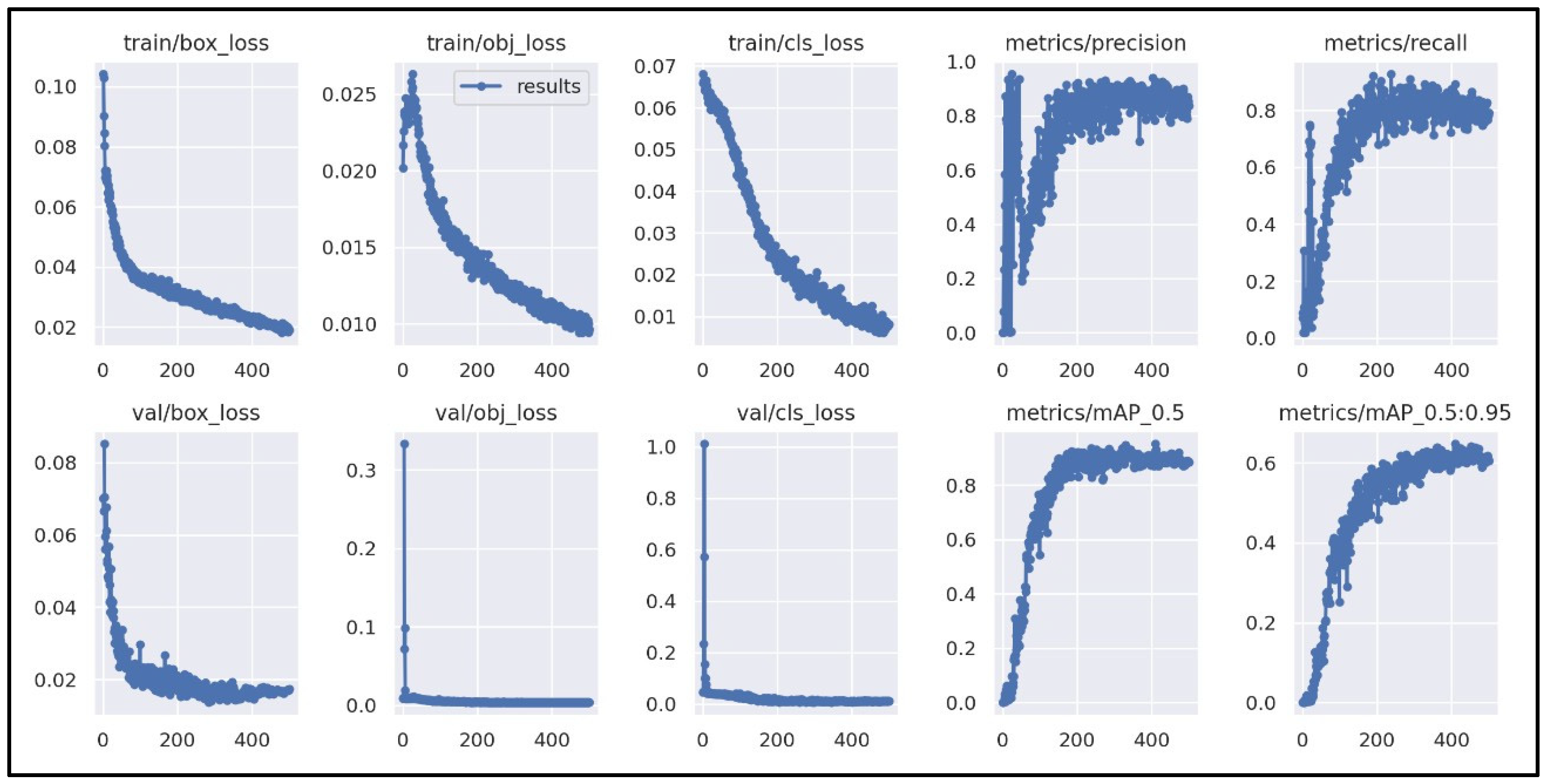
Figure 10 tracks the YOLOv5 model’s convergence; it is imperative to take into consideration the box loss (box_loss) and the classification loss (cls_loss) for both the training dataset and the validation dataset. The box_loss metric indicates that the model is steadily improving at generalization and providing better bounding boxes around the identified object, and the cls_loss metric shows that the anticipated bounding boxes are being classified well. Overall, a consistent performance is observed as the model is seen to converge.

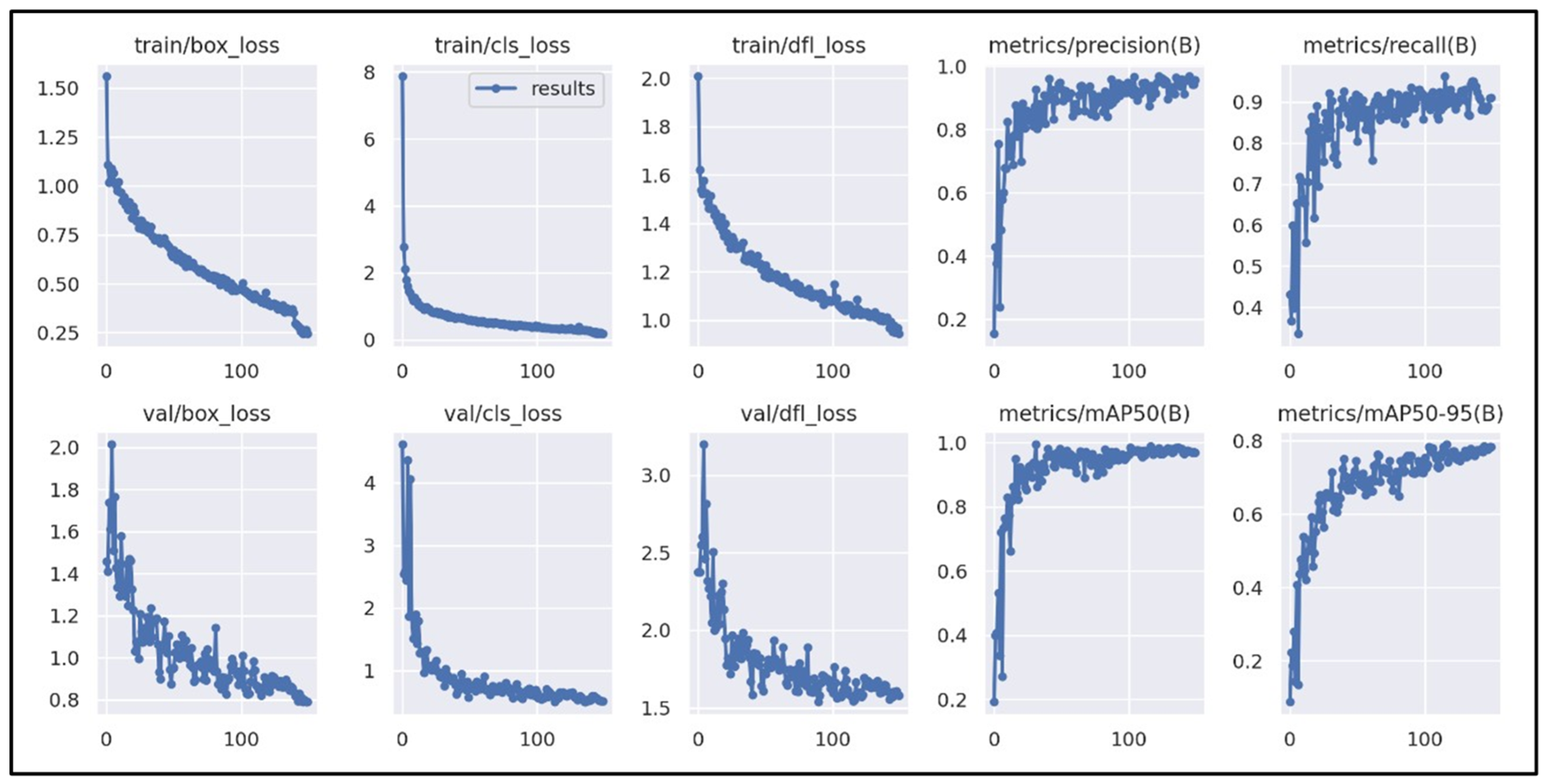
Figure 11 illustrates the metrics tracked during the training process. To assist with tracking the model’s convergence, it is imperative to take into consideration the box loss (box_loss) and classification loss (cls_loss) for both the training and the validation dataset. It is seen that the classification loss begins at a large value and steadily falls to a value less than 1, as the algorithm learns up until a point where the network is regarded to be trained and, in most cases, a lower loss percentage indicates that the model was trained more effectively.

Using the box_loss metric, the closeness of the model’s predicted bounding boxes to the actual objects in the dataset is assessed. This metric has a low value close to 0, which indicates the model is steadily improving at generalization and providing better bounding boxes around the objects that have been identified in the dataset. The performance is consistent because, at 150 epochs, the models are observed to converge.

For training these kinds of algorithms, one common approach is to divide the dataset into several groups, each containing n images, and conduct training on each group separately. This is performed in batches since sending many images to the neural network simultaneously can result in the model learning a significant number of weights in a single epoch.

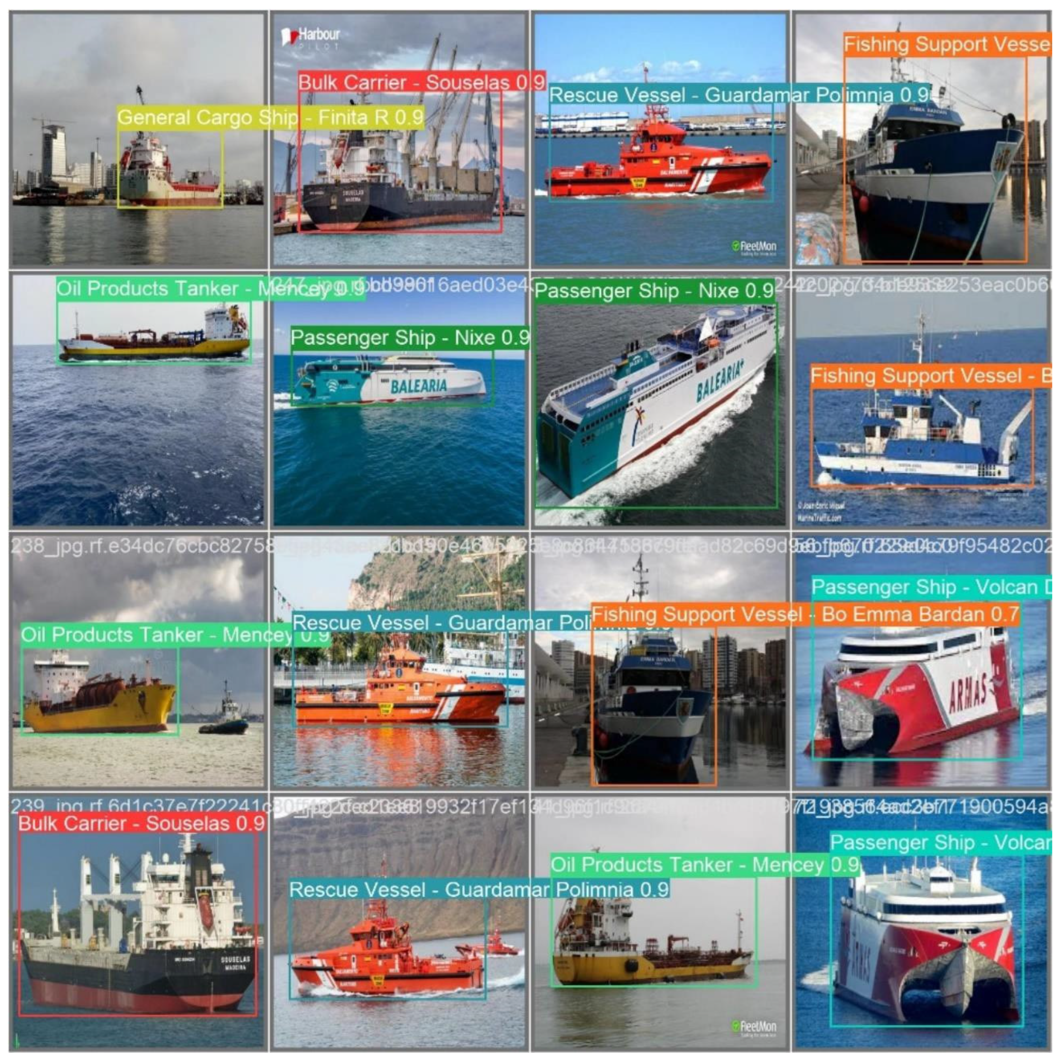
Figure 12 and Figure 13 show the predictions made by the YOLOv5 and YOLOv8 model respectively, based on the dataset that is being validated. These images were not used during the training process but are currently being used to validate the model, ensuring it is functioning as expected. A high confidence level greater than or equal to 0.9 in prediction is attained, which demonstrates that the model is high-performing and accurately classifies vessels. In the case of YOLOv5, all but one of the vessels were correctly identified and classified at a high confidence level except for the 10th image, which displays a misclassification of a general cargo ship as a cement carrier. Overall, the model is high-performing and accurately classifies vessels.

4. Results and Discussion

The tested algorithms have shown to offer good capabilities for the detection of vessels, distinguishing the different types selected. In addition, they allow the detection of vessels in a short time, thus verifying the possibility of using them in real time.

To illustrate the results of the implementations, several graphs are shown. In these graphs, all the metrics defined before are shown, so the performance of the algorithms can be evaluated through the values of the metrics.

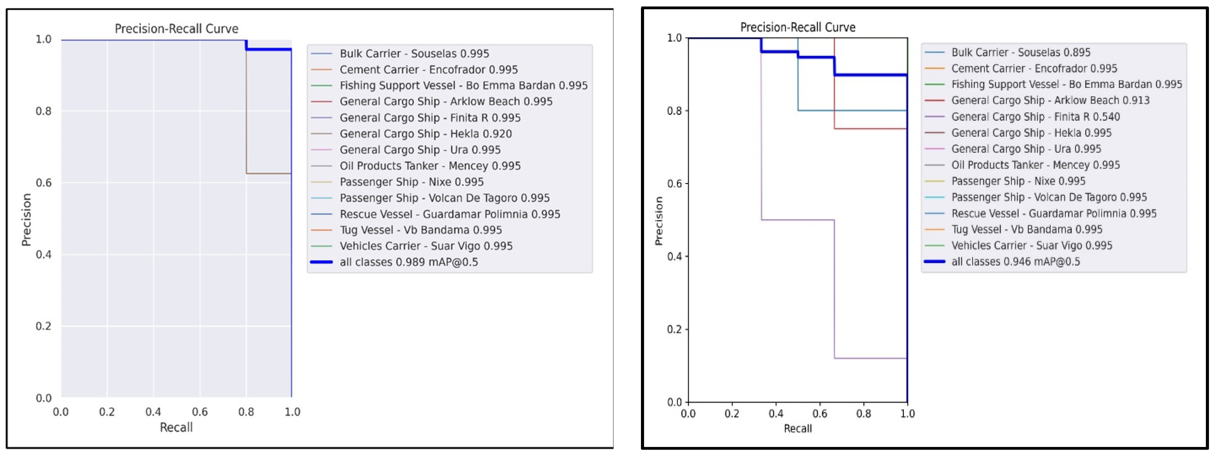
Figure 14 shows the relationship between the precision–recall curve (PRC) for YOLOv5 and YOLOv8 implementation. Precision is represented on the y-axis, and recall is plotted on the x-axis. PRC curves that are perfect traverse through the upper-right corner of the graph, where both accuracy and recall are 100%. According to Figure 14, in the case of YOLOv8 at 50% mAP, 12 of the 13 classes obtain a PRC value of 0.995, while the 13th class achieves a PRC of 0.920, and this is a satisfactory outcome. Similarly, YOLOv5 presents the perfect PRC curves traveling through the upper right corner of the graph, where both accuracy and recall are at 100%. This demonstrates that at 50% mAP, 10 of the 13 classes have a PRC of 0.995, while the remaining 3 classes range between 0.540 and 0.913, and the vessel general cargo ship Finita R is observed to perform adequately.

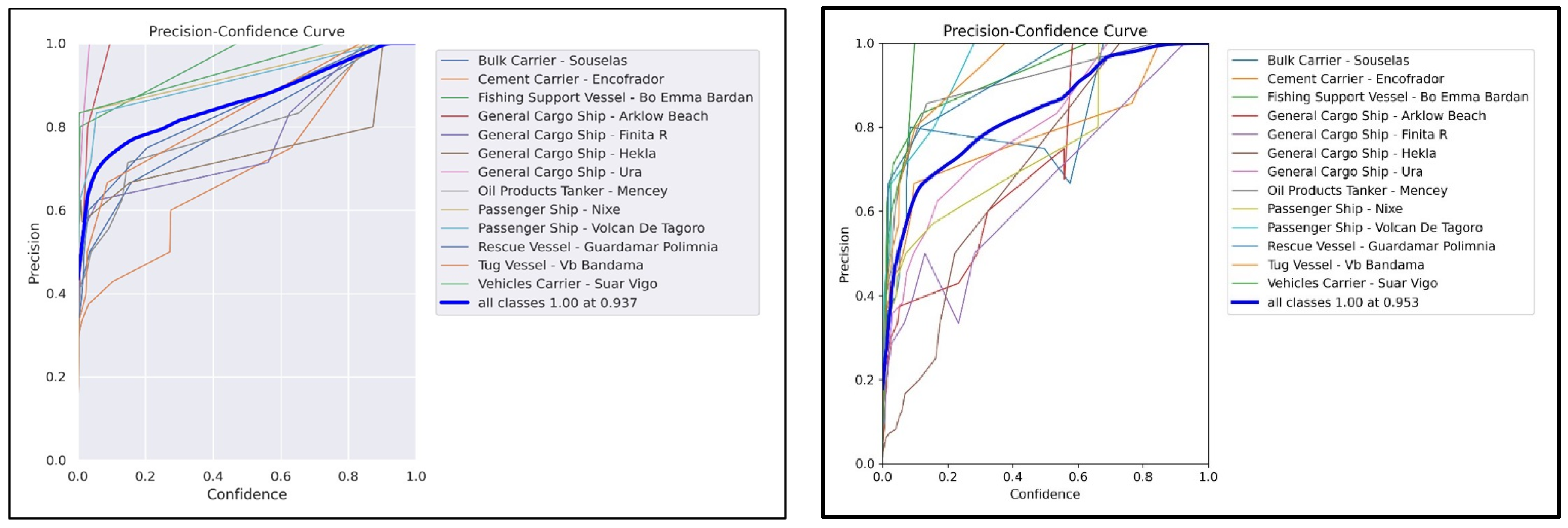
Figure 15 describes the relationship that exists between the precision of the dataset and the corresponding confidence level (PCC curve). In both cases, the graph gradually increases until it reaches its peak at 1.00 accuracy and 0.937 confidence, and this is stable.

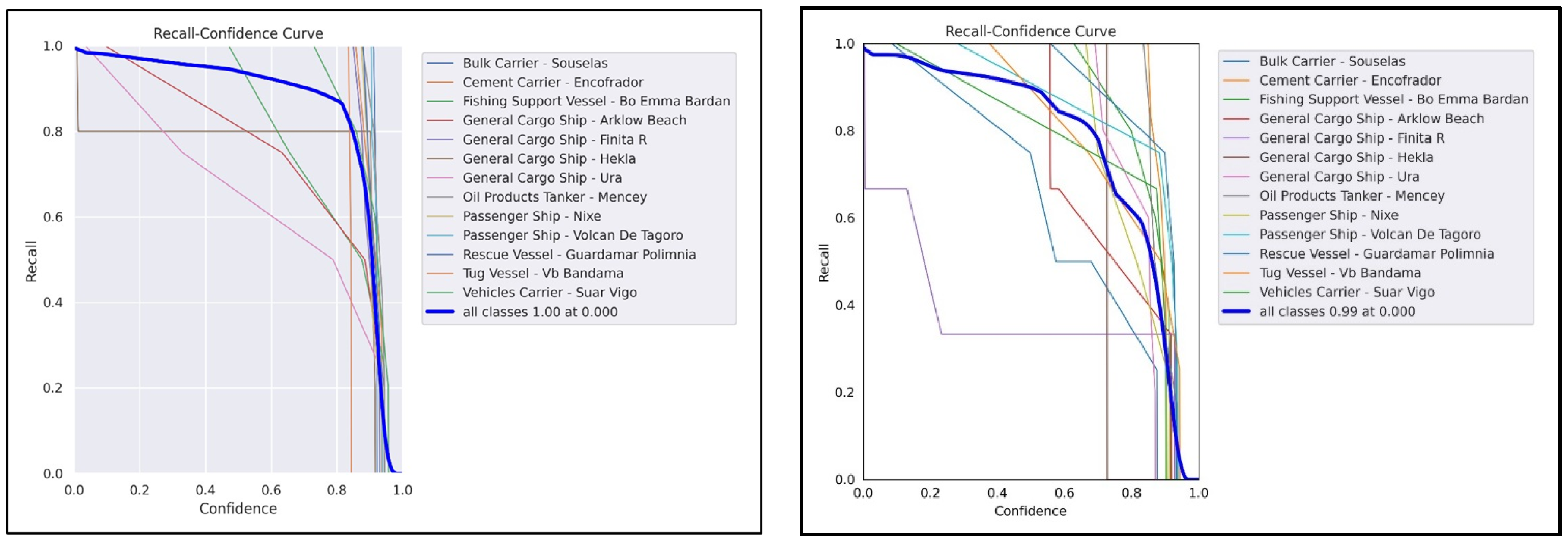
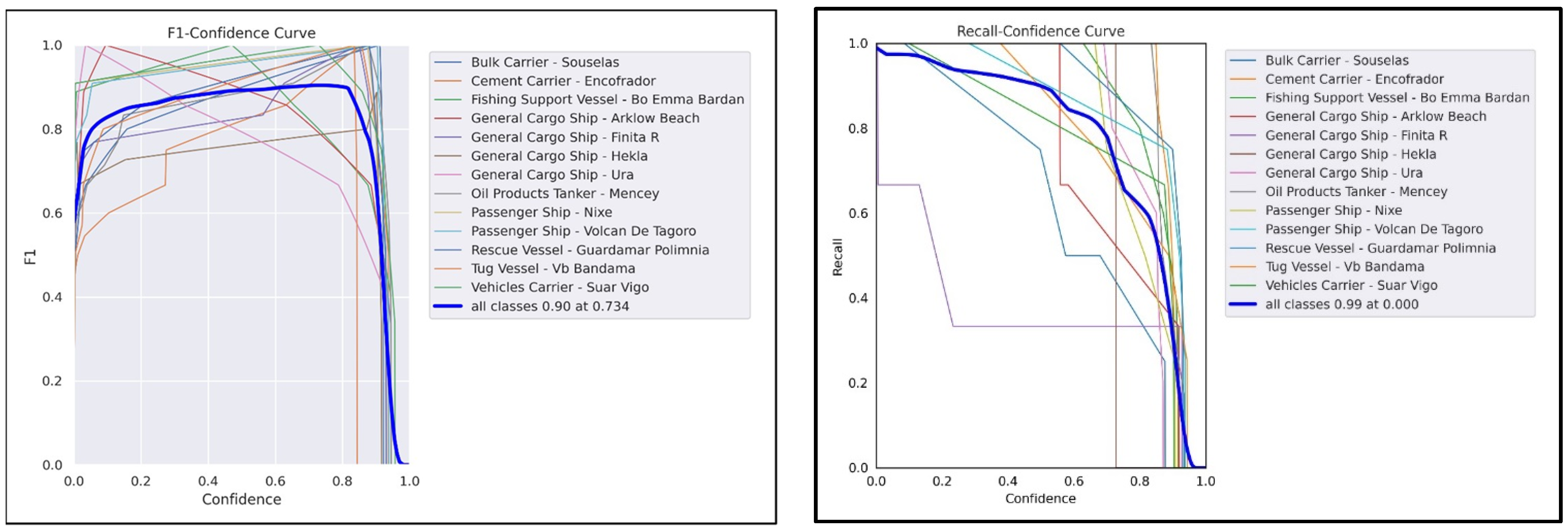
The recall–confidence curve (RCC) shows the relationship between the recall of the dataset and the confidence. In both algorithms, both metrics have been shown to have a relationship that is inversely proportional to one another (see Figure 16).

The graph of the YOLOv8 F1–confidence curve illustrates how well the F1 score relates to the confidence level of the dataset. In accordance with the F1–confidence curve, the best F1 score is 0.90, at a confidence threshold of 0.734 (see Figure 17).

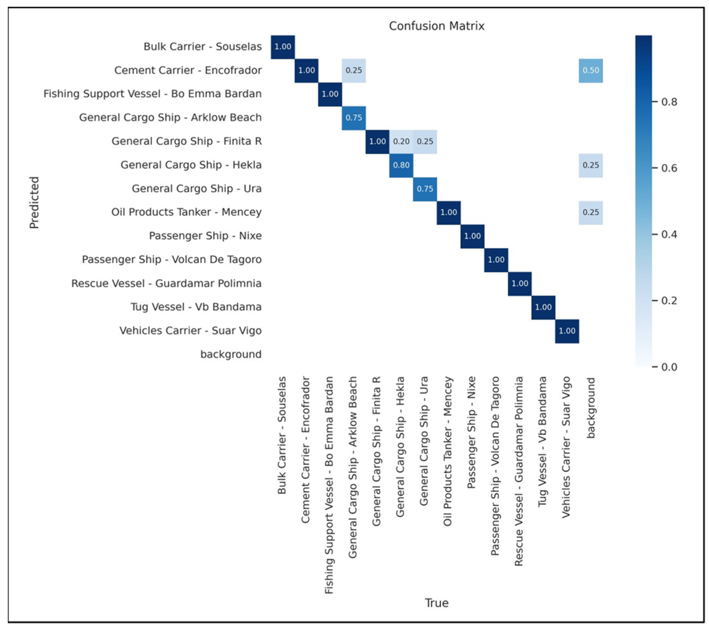
Figure 18 below is the confusion matrix, which provides information on how the model handles all 13 different classes of images during vessel detection.

To gain a deeper understanding, the matrix will be denoted as M and each element within it as M_ij. In this notation, “i” will stand for the row that represents the predicted class, and “j” the column that represents the true class. The diagonal elements M_ii and M_jj are cases of images that have been identified and classified accurately. In the case of M₄₄, the vessel is detected correctly and classified as Arklow Beach, a general cargo ship, 75% of the time. However, 25% of the time, the vessel is incorrectly classified as Encofrador, a cement carrier, even though the bounding box was successfully obtained. The rationale for this is that both have an identical physical structure and a matching color pattern.

Therefore, both models perform well in terms of identification and classification while showing distinctive qualities. However, in terms of accuracy, storage usage, and speed, the YOLOv8 model outperforms YOLOv5. So, for users who require the implementation of the most precise model and who prioritize precision over all other requirements and have enough storage capacity, the YOLOv8 model achieves better results. In the experiment, YOLOv8 achieved a mAP@50 of 98.9% and a precision of 93.9%. Although it takes an important percentage of GPU RAM, it is a precise model.

Apart from that, the YOLOv8 model is also recommended for real-time deployment because it has demonstrated a higher fps of 87.719 compared to YOLOv5’s fps of 84.745, making the first one suitable for real-time applications where speed is a critical factor. In other words, the higher the fps value, the more frames the model can process and the faster the detection process. Furthermore, although YOLOv8 had an important GPU memory usage of 7.48 Gb compared to YOLOv5’s GPU memory usage of 1.99 Gb, this value is still within acceptable limits for most modern GPUs.

YOLOv8 and YOLOv5 are both iterations of the YOLO object detection framework, with YOLOv8 being developed as an evolution beyond YOLOv5. However, the specific details about the performance comparison between YOLOv8 and YOLOv5 depend on the datasets used, the evaluation metrics, and the specific objectives of the comparison. In

Table 1. Comparison of metrics between YOLOv8 and YOLOv5.

HYPERPARAMETERS	UOM	YOLOv8	YOLOv5
mAP@50	%	98.9	95.2
mAP@50-95	%	78.8	64.0
Precision	%	0.939	0.860
Recall	%	0.895	0.892
F1 score (accuracy)	%	0.916	0.876
Weight decay	-	0.0005	0.0005
Mini-batch size	-	16	16
Training time	hours	0.37	0.533
Inference speed per image	ms	11.4	11.8
Frames per second	fps	87.719	84.745
GPU memory usage	Gb	7.48	1.99

, we show the metrics that clearly demonstrate the outperformance of YOLOv8 over YOLOv5.

The better performance of YOLOv8 compared to YOLOv5 is based on certain details, such as the following:

• Architectural Changes: YOLOv8 introduced architectural changes, such as using CSPDarknet53 as the backbone. This architecture impacts the model’s ability to capture features and representations, leading to improved performance. In this work, we are interested in capturing features of the ship’s superstructure that help identify the type of ship. However, a lightweight improved YOLOv5 is proposed in [34] for real-time localization of fruits, using the bneck module of MobileNetV3 instead of CSPDarknet53. In this study, the modified YOLOv5 reached the mAP of 0.969.
• Training Techniques: YOLOv8 incorporated training techniques, such as the use of CIOU (complete intersection over union) loss and focal loss. These techniques are aimed at improving the accuracy of object detection during the training process.
• Scales for Flexibility: YOLOv8 provides different scales (S, M, L, and X). This allows us to choose the scale that best fits our requirements. This adaptability was beneficial for customizing the models to the specific task of detecting ship profiles.
• Task Adaptability: YOLOv8 is designed to be adaptable to various object detection tasks, including custom applications. The architecture allows us to train models on our specific datasets.

In this approach, the most interesting feature is to obtain the fastest model for real-time deployment. In this case, YOLOv8 demonstrated a higher fps (frames per second) of 87.719 compared to YOLOv5’s fps of 84.745, making it better suited for real-time applications where speed is a critical factor. In other words, the higher the fps value, the more frames the model can process and the faster the detection process. Furthermore, while YOLOv8 had a higher GPU memory usage of 7.48 Gb compared to YOLOv5’s GPU memory usage of 1.99 Gb, this value is still within acceptable limits for most modern GPUs. Hence, YOLOv8’s higher fps value and acceptable GPU memory usage make it the best option for real-time deployment above all other factors.

It is important to note that the performance of YOLOv8 compared to YOLOv5 can vary based on the evaluation criteria and the specific datasets used for testing; that is, dataset size, diversity, and the nature of the recognition problem. The same happens if you compare YOLO performance with generic CNNs for image recognition. This task typically involves classifying entire images into predefined categories, whereas YOLO is specialized for object detection, where the goal is to locate and classify multiple objects within an image.

5. Conclusions

This research had the goal of tackling an environmental problem. We must develop a system to gather plastic garbage that is floating over the water. For this, a containment system is proposed. This system consists of a conventional barrier, but it is necessary to modify it due to the passage of ships through the area (rivers, canals, access to ports, etc.).

We proposed the developing of an autonomous system to address the efficient movement of a conventional barrier when a ship is going to pass through it. An important part of this is detecting the approach of the ship, the type of ship and the approaching speed. For this detection and classification we compared YOLO algorithms.

This detection triggers the order for the mechanical system of the barrier to immersion. This process consists of flooding the interior of the barrier as ballast and generating a layer of bubbles that take the place of the conventional barrier so that the garbage accumulated up to that moment is not dispersed. Once the ship leaves the barrier zone, the process is reversed. The conventional barrier is emptied of water, and it emerges to the surface, once again containing the garbage. Currently, the bubble barrier is deactivated.

To achieve this goal, we conducted an in-depth analysis of computer vision models for use within the marine field, with a focus on vessel recognition, classification, and data provision. For the identification and classification phase, we have demonstrated the usage of two detection frameworks, YOLOv8 and YOLOv5, which were trained, analyzed, and tested on a dataset and measured using a set of hyperparameters.

As we said in the literature review, some previous works [9] stated that ship detection algorithms based on convolutional neural networks achieved good results, albeit with many missed and false detections.

Table 2. Comparison of metrics between different algorithms.

Method	Precision (%)	Recall (%)	mAP (%)
Faster R-CNN (Yu and Shin)	78.49	81.42	79.33
RetinaNet (Yu and Shin)	82.16	83.35	81.14
YOLOv5 (Yu and Shin)	83.02	84.97	82.26
YOLOv5 (ours)	86.0	89.2	95.2
YOLOv8 (ours)	93.7	89.5	98.9

below shows a comparison between the results in [9] and our results.

Even though [9] worked with radar images of ships and we worked with images of ships’ fronts, the YOLO architecture is very similar in both works. They used a CSPDarkNet53 as the backbone network and an SPP (spatial pyramid pooling) layer, as we did. This layer uses maximum pooling methods with four different sizes to significantly increase the receptive fields. The idea of the cross-stage partial network (CSP) is to integrate the gradient change into the feature map from the beginning to the end, reducing the network parameters and the amount of computation. Therefore, the goal of both works is to improve the detection accuracy while maintaining the running speed by stacking convolution modules. YOLOv8 introduces several improvements over previous versions in terms of its control scheme, which enhances the overall performance, usability, and flexibility of the model. These improvements are designed to optimize the model’s training and inference processes, making it more robust and efficient. The proposed control scheme introduces a neck design that is more robust to variations in object scale and shape, an improved detection head with more accurate bounding boxes and class prediction, and enhanced loss functions that better handle class imbalance and improve the learning process. These improved features were needed to tackle the problem of ship detection in real-time by using ship profile images that can be captured from different perspectives. The improved architecture of YOLOv8 demonstrated a quantitative increase in accuracy.

Therefore, the research objectives have been fulfilled; however, it is probable that a more definitive conclusion would have been obtained if the following had not been encountered. First, access to the necessary data was a limitation that had to be resolved during this research. The vessel data had to be gathered manually, and there were only a few resources that allowed public access to both the vessel image and its data. This was a limitation, and as a result, the number of vessels of each class that could be used for the project was limited.

Another issue that needed to be addressed was the requirement to choose between images with high and low resolutions rather than only images with high resolutions. To avoid class imbalance, misidentified and misclassified vessels, this option necessitated a trade-off during the data processing step. As a result, the original dataset had to be scaled down to avoid using low-quality images.

The findings in this study highlight the trade-offs between the two models, guiding the selection based on specific application needs and resource availability. YOLOv8’s enhancements make it a compelling choice for accuracy-critical tasks, particularly for vessel detection and classification tasks, while YOLOv5 remains practical for applications requiring efficient use of computational resources.