Article

Intelligent Detection of Marine Offshore Aquaculture with High-Resolution Optical Remote Sensing Images

1
South China Sea Institute of Planning and Environment Research, State Oceanic Administration, Guangzhou 510300, China
2
Key Laboratory of Marine Environmental Survey Technology and Application, Guangzhou 510300, China
3
Technology Innovation Center for South China Sea Remote Sensing, Surveying and Mapping Collaborative Application, Ministry of Natural Resources, Guangzhou 510300, China
4
School of Surveying and Urban Spatial Information, Henan University of Urban Construction, Pingdingshan 467036, China
*
Authors to whom correspondence should be addressed.
These authors contributed equally to this work.
J. Mar. Sci. Eng. 2024, 12(6), 1012; https://doi.org/10.3390/jmse12061012
Submission received: 7 May 2024 / Revised: 1 June 2024 / Accepted: 13 June 2024 / Published: 18 June 2024
(This article belongs to the Special Issue Sustainable Development and Resource Management of Marine Aquaculture)

Abstract

:
The rapid and disordered expansion of artificial marine aquaculture areas has caused severe ecological and environmental problems. Accurate monitoring of offshore aquaculture areas is urgent and significant in order to support the scientific and sustainable management and protection of coastal marine resources. Artificial intelligence provides a valuable tool to improve marine resource monitoring. Deep learning methods have been widely used for marine object detection, but You Only Look Once (YOLO) models have not been employed for offshore aquaculture area monitoring. This study therefore evaluated the capacity of two well-known YOLO models, YOLOv5 and YOLOv7, to detect offshore aquaculture areas based on different high-resolution optical remote sensing imagery. Compared with YOLOv7 based on a satellite dataset, YOLOv5 increased the Precision value by approximately 3.29% (to 95.33%), Recall value by 3.02% (to 93.02%), mAP_0.5 by 2.03% (to 96.22%), and F1 score by 2.65% (to 94.16%). Based on the Google Earth dataset, YOLOv5 and YOLOv7 showed similar results. We found that the spatial resolution could affect the deep learning models’ performances. We used the Real-ESRGAN method to enhance the spatial resolution of satellite dataset and investigated whether super-resolution (SR) methods improved the detection accuracy of the YOLO models. The results indicated that despite improving the image clarity and resolution, the SR methods negatively affected the performance of the YOLO models for offshore aquaculture object detection. This suggests that attention should be paid to the use of SR methods before the application of deep learning models for object detection using remote sensing imagery.

1. Introduction

Over the past few decades, China has witnessed extensive developments in the marine aquaculture industry [1], with the total output value of fisheries increasing from RMB 41.056 billion in 1990 to RMB 1526.749 billion in 2022. The rapid and disordered expansion of artificial marine aquaculture areas has caused severe ecological and environmental problems, such as water pollution [2,3], biodiversity degradation [4], nature wetland loss [5], marine traffic obstruction, etc. It is significant and urgent to accurately monitor offshore aquaculture areas to support the scientific and sustainable management of marine aquaculture resources [1,3].
Remote sensing has been widely used for dynamic monitoring of offshore aquaculture for decades [6,7,8]. Researchers initially relied on visual interpretation to monitor offshore aquaculture areas, which was time-consuming, labor-intensive, and heavily reliant on the expertise of interpreters [9,10,11]. With massive quantities of remote sensing data accumulated every year, artificial intelligence is required to meet the increasing demand for food and the expansion of offshore aquaculture [12]. Machine learning (ML) techniques, including support vector machines, decision trees, random forest, and genetic programming, have been utilized in offshore aquaculture monitoring [7,13,14]. ML has great robustness in handling large or complex feature spaces [15] and can obtain reliable classification accuracy even without feature selection. Researchers have proposed new features to detect offshore aquaculture areas. Wang et al. [16] presented an object-based visually salient Normalized Difference Vegetation Index (NDVI) feature and achieved good detection results with Gaofen-2 spectral imagery. Liu et al. [13] combined an object-oriented Normalized Difference Water Index (NDWI) and edge feature extraction to detect raft and cage aquaculture areas in China with Landsat-8 imagery. Wang et al. [17] proposed an optical remote sensing aquaculture index, the Marine Aquaculture Index (MAI), and designed a random forest-based extraction scheme to detect cage and raft aquaculture areas in the Bohai Rim using time series Sentinel-1 and Sentinel-2 satellite imagery. Wang et al. [18] combined multi-scale feature fusion and spatial rule induction to extract raft cultivation areas using high-spatial-resolution remote sensing imagery. It should be pointed out that ML requires considerable engineering and domain expertise to design a feature extractor that transforms raw data to features, such as spectral, textural, geometric relationship characteristics, so that the classifier can detect and classify different land covers [19,20]. Thus, for ML, defining features is necessary and multiple adjustments are required to achieve favorable results [21,22].
Deep learning methods eliminate the need for the prior definition of features and offer advantages such as robust feature extraction and the ability to handle complex scenarios [23]. Requiring little work by hand, deep learning can take advantage of increases in the accessible computational processing power and the amount of remote sensing data [19]. Researchers have explored the recognition and generalization ability of semantic segmentation deep learning models, such as DeepLab-v3+, U-Net, and convolution neural networks, to detect marine aquaculture areas [1,24]. Some researchers have even proposed new deep learning methods for aquaculture area extraction. Chen et al. [20] proposed a new lightweight fully connected spatial dropout network (LFCSDN), combining U-Net and DeepLab-v3+ feature fusion strategies to detect floating raft aquaculture areas. LFCSDN achieved an optimal F1 score of 94.04%, surpassing U-Net (91.64%) and DeepLab-v3+ (91.66%) [20]. Deng et al. [25] proposed a coastal aquaculture network based on GaoFen-2 satellite images to extract information about cage and raft aquaculture areas in mainland China, with overall accuracy of 94.64%.
In addition to semantic segmentation methods, many researchers have recently utilized object detection deep learning methods involving YOLO (You Only Look Once) algorithms to identify and localize objects in the ocean [26,27,28,29,30,31,32,33,34,35]. The first generation YOLO model was developed by Redmon et al. [36] in 2016 and was subsequently enhanced [37]. Hong et al. [38] proposed an improvement on YOLOv3 for marine ship detection based on SAR and optical satellite imagery with different scales, which showed high average precision with optical imagery (93.56%) and SAR imagery (95.52%) [38]. Based on YOLOv4 network architecture, Hu et al. [39] proposed a novel small-ship detection method, termed as portable attention-guided YOLO (PAG-YOLO) algorithm. The PAG-YOLO could obtain high average precision (91.00%) with the public MASATI (Maritime Satellite Imagery) dataset [39]. Chen et al. [40] presented a complex scenes multi-scale ship-detection model (CSD-YOLO) to detect ships in SAR images. With the public High-Resolution SAR Images Dataset (HRSID) and a SAR Ship-Detection Dataset (SSDD), the CSD-YOLO model achieved 98.01% detection accuracy, 96.18% Recall, and a mean average precision of 98.60% on SSDD, outperforming other methods [40].
Although YOLO models have been widely and successfully used in marine object detection, they have not previously been employed for the recognition of offshore aquaculture areas. Super-resolution (SR), which obtains high-resolution images from low-resolution observations, has been a popular research topic in image processing fields and has been employed widely [41]. The specific objectives of this study are as follows: (1) to evaluate the capacity of YOLOv5 and YOLOv7 for offshore aquaculture detection based on different high-resolution optical remote sensing images; (2) to assess whether SR methods can improve the offshore aquaculture detection accuracy of YOLO models. The remainder of this article is arranged as follows. Section 2 presents the study area and data. Section 3 describes the methods used in this study. Section 4 presents the results and discussion. Section 5 summarizes the major conclusions.

2. Study Area and Data

2.1. Overview of the Study Area

The study area was Zhelin Bay, the largest mariculture base in southern China, located in Raoping County, in the northeast of Guangdong Province (Figure 1). Guangdong Province is one of the most economically developed provinces in China and also has the largest aquaculture production [42]. Zhelin Bay covers an area of about 70 km2 [43], with an average water depth of 4.8 m, and a maximum water depth of 12 m. It is the largest marine aquaculture area in eastern Guangdong [44]. Within this area, cage aquaculture accounts for 13.4 km2 [45]. The marine aquaculture in Zhelin Bay has played a positive role in promoting local economic development but has led to rapid declines in the aquatic ecosystem in recent years [42,43,46].

2.2. Data

2.2.1. Google Earth Imagery Dataset

We obtained Google Earth imagery from 2019 to 2021, with spatial resolution varying from 0.5 m to 1 m in the study region. The three types of offshore aquaculture areas on the Google Earth imagery were named as cage, raft, and deep-sea cage aquaculture areas (Figure 2).

2.2.2. Satellite Imagery Dataset

We utilized satellite imagery of the study region acquired via the Gaofen-1B satellite on 3 November and 14 December 2019, the Gaofen-6 satellite on 9 April 2020, and the ZY-3 02 satellite on 16 March 2020. The key parameters of the satellite camera systems are listed in Table 1. The four categories of the offshore aquaculture areas on the satellite imagery were named as cage, raft, deep-sea cage, and cage-2 aquaculture areas (Figure 3). It should be pointed out that due to the different spatial resolutions of the satellite imagery, we classified two different categories of cages based on the satellite imagery dataset.
To enhance the spatial resolution of the multispectral satellite imagery, we employed the pan-sharpening method to fuse the geometrically corrected multispectral and panchromatic images and obtained multispectral data with four bands at 2 m spatial resolution. Furthermore, to enhance the spectral contrast between the offshore aquaculture areas and the surrounding terrain and water in the study region, we selected infrared, red, and green bands for the RGB band combination (Figure 1). As the spatial resolution of the processed satellite imagery was lower than that of the Google Earth imagery, we further used super-resolution methods to enhance the spatial resolution of the satellite imagery.

2.2.3. SR-Augmented Satellite Imagery Dataset

SR is a task in computer vision that converts low-resolution images to high-resolution images. It has been widely applied in image and video processing to improve image quality and visual details and increase the accuracy of computer vision algorithms [47]. ESRGAN (enhanced super-resolution generative adversarial network) is a deep learning technique for SR. ESRGAN is based on the traditional SR algorithm SRGAN and introduces a structure known as residual blocks to further improve the image quality [48]. The ESRGAN technique has demonstrated excellent performance in remote sensing image processing [49,50].
Real-ESRGAN is a practical application extended from ESRGAN [51]. We applied the official Real-ESRGAN x4plus model [52] to enhance the resolution of the collected satellite imagery. This method increased the image resolution with a scaling factor of 4; the spatial size of the satellite imagery increased from 600 × 600 to 2400 × 2400. Then, we compressed the spatial size of the images to 640 × 640 to accommodate the parameters of the YOLOv5 and YOLOv7 algorithms. The four categories of offshore aquaculture areas on the SR augmented satellite imagery are shown in Figure 4. We can see the improved clarity of the different aquaculture types on the SR-augmented satellite dataset (Figure 3 and Figure 4).

2.3. Data Augmentation

In this study, we first obtained the sample data using the visual interpretation method based on the Google Earth dataset, satellite dataset, and augmented satellite dataset. Deep learning models rely heavily on big sample data to avoid overfitting, while data augmentation can enhance the size and quality of sample data and improve the robustness of the model [53]. Thus, we augmented the three sample datasets with data augmentation algorithms, including flip, 90-degree rotations, hue change, saturation change, brightness change, and mosaic. These data augmentation algorithms were employed using the Roboflow website (https://roboflow.com/ (accessed on 1 December 2023)). The details of the augmentation algorithms are listed as follows:
(1)
Flip: the array of the image was flipped vertically.
(2)
90-degree rotation: the image was rotated 90 degrees clockwise or counterclockwise.
(3)
Random rotation: the image was rotated around the centroid with a rotation degree randomly chosen from [0, 30].
(4)
Change hue: a randomly selected degree of hue enhancement from the range [–15, 15] was applied to the image.
(5)
Change saturation: a randomly selected saturation enhancement value from the range [−15, 15] was applied to the image.
(6)
Change brightness: a randomly selected a brightness enhancement value from the range [0, 15] was applied to the image.
(7)
Mosaic: four different training images were combined in a mosaic.
After data augmentation, each of the Google Earth, satellite, and SR-augmented satellite dataset consisted of 1300 samples with 640 × 640 pixels. Each dataset was randomly divided into the corresponding training and validation datasets with a ratio of 9:1. The training dataset consisted of 1170 samples, while the validation dataset consisted of 130 samples. The augmented image samples are shown in Figure 5. Tao et al. [54] and Ma and Zhang [55] found that the detection accuracy could be greatly improved using a ratio of 9:1 for the training and validation sample datasets.

3. Methods

3.1. Models

This study employed the YOLOv5 and YOLOv7 algorithms to detect offshore aquaculture areas. YOLOv5 and YOLOv7 are state-of-the-art object detection algorithms [56,57,58,59]. The YOLOv5 method demonstrates superior performance in both accuracy and speed compared with previous YOLO versions, while the subsequently released YOLOv7 also shows good performance [56,58]. Therefore, this study selects these two algorithms for comparative analysis and evaluation.

3.1.1. YOLOv5

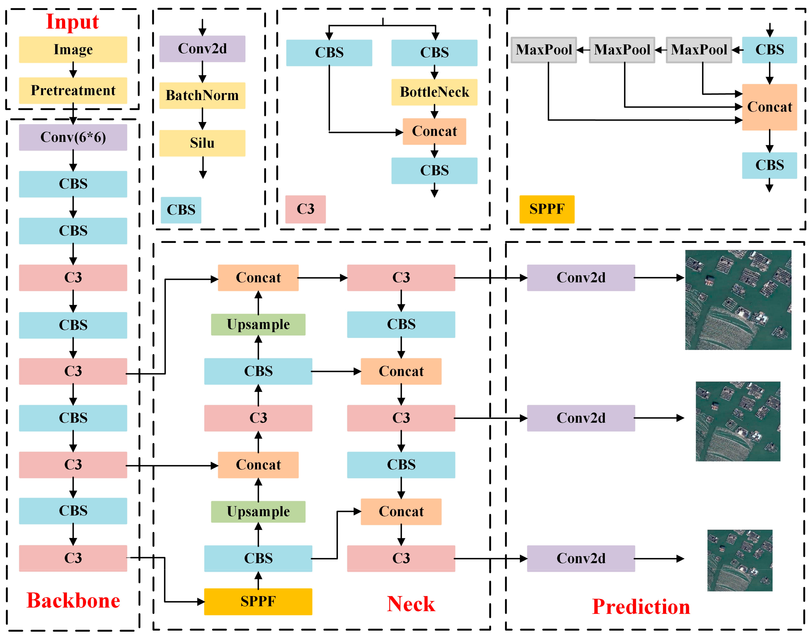
Ultralytics released YOLOv5 in May 2020 [60]. We used the v6.2 YOLOv5 model in this study [61]. The architecture of the YOLOv5 model is illustrated in Figure 6. The YOLOv5 model comprises four parts: input layer, backbone layer, neck layer, and prediction layer.
YOLOv5 has four network structures of various depths and widths, including YOLOv5s, YOLOv5m, YOLOv5l, and YOLOv5x. YOLOv5s has the smallest depth and width with the fastest speed, while YOLOv5x has the largest depth and width but runs more slowly. We tested the four network structures with sample data and found that YOLOv5x showed the best offshore aquaculture detection performance. Regarding the hyperparameters in the model, we tried to change the hyperparameters and evaluate the detection accuracies, and we found that YOLOv5x with the default hyperparameters preformed the best. Thus, in this study, we used YOLOv5x with the default hyperparameters for offshore aquaculture detection [60].

3.1.2. YOLOv7

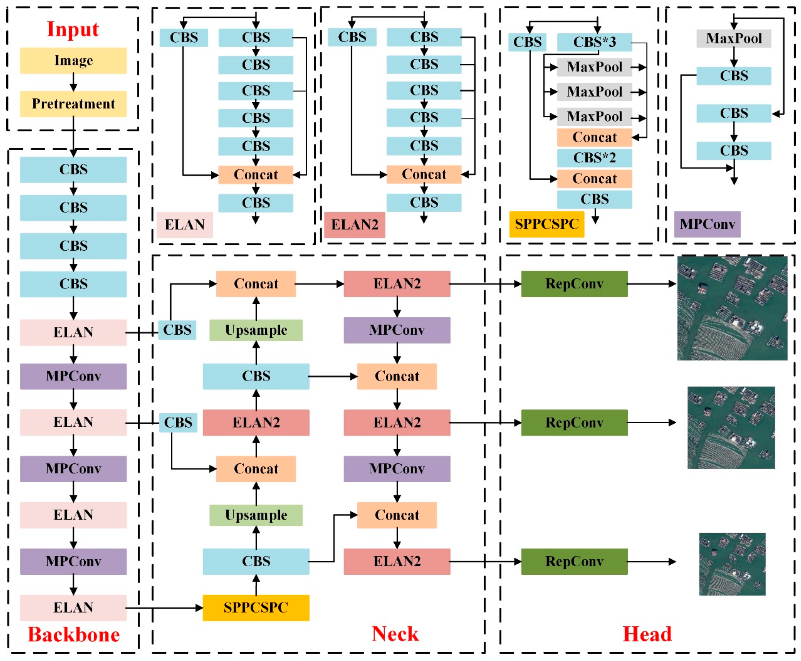
In July 2022, the YOLOv4 development team led by Alexey Bochkovskiy released YOLOv7, which has demonstrated outstanding performance in various applications [40,59]. The network architecture of YOLOv7 is depicted in Figure 7. The YOLOv7 model also comprises four parts: input layer, backbone layer, neck layer, and head layer. YOLOv7 has four network structures of various depths and widths, including YOLOv7s, YOLOv7m, YOLOv7l, and YOLOv7x. Through comparison and analysis, we selected YOLOv7x [62] with the default hyperparameters for offshore aquaculture detection in the current study.

3.2. Experiment Environment

In this study, all experiments were implemented in PyTorch on a PC with Intel(R) Core(TM)2 Duo CPU T7700 @ 2.40GHz, NVIDIA GRID RTX8000-48Q GPU. The PC operating system was Windows 10. The computer and deep learning environment configuration for our experiments are described in Table 2.

3.3. Model Parameters

In the training stage, the model parameters were the default pre-trained weights of the YOLOv5x [60] and YOLOv7x [62] models. Both models were trained for 200 epochs with a batch size of 8. In the prediction stage, we employed the weights obtained from the training stage.

3.4. Performance Evaluation

We used Precision, Recall, mean average precision (mAP), and F1 score to evaluate the model’s performance. A validation test employing a tenfold cross-validation method was applied to calculate the evaluation metrics, and the performance metric for the model was the average of the tenfold cross-validation data [63].
Precision is one of the most common evaluation indexes, and refers to the number of correct targets divided by the number of detected targets. Precision, Recall, mAP, and F1 score were calculated as follows:
P r e c i s i o n = T P T P + F P
R e c a l l = T P T P + F N
A P = 0 1 P R d R
m A P = 1 N i = 1 N A P ( i )
F 1 = 2 × P r e c i s i o n × R e c a l l P r e c i s i o n + R e c a l l
where TP (true positive) corresponds to the number of offshore aquaculture targets that are correctly detected; FP (false positive) represents the number of other objects detected as offshore aquaculture targets; FN (false negative) represents the number of offshore aquaculture targets that are undetected or missed [59,64].
AP (Average precision) is a metric in measuring the accuracy of object detectors. AP computes the average precision value for recall values over 0 to 1. mAP is the average of AP. F1 score is a weighted average of precision and recall values, and ranges from 0 to 1. F1 score reflects the model’s overall precision and recall performance.
Confidence is crucial for assessing the model’s object detection accuracy. It indicates both the likelihood of an object’s presence in the detection box and the model’s confidence in this assessment. Confidence is defined as Pr O b j e c t × I O U p r e d i c t i o n t r u t h , with the score being zero if no object is detected [36].
P r c l a s s i O b j e c t × P r O b j e c t × I O U p r e d i c t i o n t r u t h = P r ( c l a s s i ) × I O U p r e d i c t i o n t r u t h
In Equation (6), Pr denotes the probability of an object’s presence, IOU (intersection of union) is the ratio of the intersection area of the actual and predicted boxes to their union area, class refers to the predicted class, Object is the object being predicted, and i is the number of classes.

4. Results and Discussion

4.1. Performance Evaluation

To evaluate the capacity of YOLOv5 and YOLOv7 for offshore aquaculture detection based on different high-spatial-resolution optical remote sensing images, we conducted six experiments based on two models (YOLOv5 and YOLOv7) and three datasets (the satellite dataset, the Google Earth dataset, and the SR-augmented satellite dataset). The YOLO model detection results are listed in Table 3. Based on the results of Experiments 1–4 (Table 3), the highest mAP_0.5 values for both YOLOv5 and YOLOv7 models all exceeded 95%, indicating the good detection performances of YOLOv5 and YOLOv7.
To reveal whether the difference of the model performance was statistically significant, we used paired t-testing on the results of the cross-validation (Table 4). In terms of Precision, mAP_0.5, and F1 score, YOLOv5 statistically outperformed YOLOv7 based on both the satellite dataset and the SR-augmented satellite dataset (Experiments 1 and 2, Experiments 5 and 6 in Table 3). This conclusion was similar to that of a previous study [65], which compared YOLOv5 and YOLOv7 with the Google Open Images dataset and Roboflow public dataset for the detection of persons, handguns, rifles, and knives. However, the Precision, mAP_0.5, and F1 values derived from YOLOv5 and YOLOv7 using the Google Earth dataset were not significantly different, suggesting that YOLOv5 and YOLOv7 produced similar results when using the Google Earth dataset (Experiments 3 and Experiment 4). In terms of Recall, YOLOv5 statistically outperformed YOLOv7 based on the satellite dataset, while the Recall values from the YOLOv5 and YOLOv7 models based on the SR-augmented satellite dataset or the Google Earth dataset were not significantly different (Table 3 and Table 4).
We also applied paired t-testing to assess the precision evaluation metrics of different datasets (Table 5). Based on the same YOLOv5 or YOLOv7 models, Recall, mAP_0.5, and F1 scores were statistically different between the Google Earth dataset and the satellite dataset, and between the satellite dataset and the SR augmented satellite dataset. Thus, in terms of Recall, mAP_0.5, and F1 score, the precision evaluation metrics of the Google Earth dataset were statistically better than the satellite dataset, and those of satellite dataset were statistically better than the SR-augmented satellite dataset (Table 3 and Table 5). The Precision values of the satellite dataset were significantly better than those of the SR-augmented satellite dataset, for both the YOLOv5 and YOLOv7 models. The Precision values of the Google Earth dataset were significantly better than those of the satellite dataset for YOLOv7, while the Precision values of the Google Earth dataset and satellite dataset were similar for YOLOv5 (Table 3 and Table 5).
Based on the SR-augmented satellite dataset (Experiment 5 and Experiment 6 in Table 3), both YOLOv5 and YOLOv7 showed a decline in precision evaluation metrics compared with the corresponding models based on the satellite dataset (Experiment 1 and Experiment 2). This indicates that applying the SR method to the satellite imagery for offshore aquaculture detection may not contribute to an improvement in the detection accuracy. Although the SR-augmented satellite dataset might have appeared visually clearer and had higher resolution (Figure 3 and Figure 4), the SR algorithm may have led to feature loss of the offshore aquaculture objects in the satellite imagery, and this adversely affected the model’s ability to accurately capture essential information about the object during training, negatively impacting the detection accuracy of the YOLO models.

4.2. FPS Comparison

Based on the same datasets, we did not find that the frames per second (FPS) values were significantly different between the YOLOv5 and YOLOv7 models (Table 4). This indicates that these two models had similar inference speed in offshore aquaculture detection. The FPS values were significantly different between the satellite dataset and the SR-augmented satellite dataset with YOLOv5, suggesting that YOLOv5 was capable of detecting aquaculture objects quicker with the satellite dataset than the SR-augmented satellite dataset (Table 5).

4.3. Object Detection Comparison

The object detection results of YOLOv5 and YOLOv7 were similar, with only minor differences in relation to some individual offshore aquaculture targets (Figure 8). To further compare the detection accuracies of the two YOLO models based on the satellite and Google Earth datasets, we averaged the confidence values of all validation samples based on YOLOv5 and YOLOv7 with the satellite and Google Earth datasets. The average confidence values of different models and datasets are displayed in Table 6. The average confidence values of YOLOv5 and YOLOv7 based on the satellite dataset were 0.90 and 0.86, respectively, and the average confidence values of YOLOv5 and YOLOv7 based on Google Earth dataset were 0.85 and 0.81, respectively. This indicates that YOLOv5 generally had statistically higher confidence value when detecting offshore aquaculture targets than YOLOv7, and both YOLOv5 and YOLOv7 based on the satellite dataset obtained statistically higher confidence values than when they were based on the Google Earth dataset. Although the Recall, F1 score, and mAP_0.5 values of the two models based on the Google Earth dataset were larger than those based on the satellite dataset (Table 3), the average confidence values of those based on the Google Earth dataset were lower (Table 6).
As the confidence value threshold (Conf_thres) may influence the object detection accuracy, we adjusted the Conf_thres values between 0.3 and 0.9 and calculated the average confidences based on different models and datasets (Table 7). For both the satellite dataset and Google Earth dataset, the average confidence value of YOLOv5 was statistically higher than that of YOLOv7. As for YOLOv5, the average confidence value based on the satellite dataset was higher than that based on the Google Earth dataset when the Conf_thres value was smaller than 0.7. For YOLOv7, the average confidence values based on the satellite dataset were higher than those based on the Google Earth dataset using the Conf_thres values from 0.3 to 0.6. These results indicated that YOLO models trained on Google Earth dataset performed well on the training dataset but poorly on the validation data, which may be due to an overfitting issue in the YOLO model training based on the Google Earth dataset [66,67,68].

4.4. Adaptability of the Models and Data

In this study, we explored the use of YOLOv5 and YOLOv7 to detect offshore aquaculture areas in Zhelin Bay. To combat the overfitting problem in deep learning models, we used transfer learning, data augmentation, regularization techniques, and early stopping. Through trial and error, we selected the YOLOv5x and YOLOv7x models with the default hyperparameters, which is transfer learning. As there were no existing aquaculture datasets available on the websites, we created the training and validation samples with the collected remote sensing imagery. Then, we used data augmentation to enhance the size and quality of the sample data. In addition, regularization techniques and early stopping within the YOLO models can also mitigate overfitting in the deep learning models.
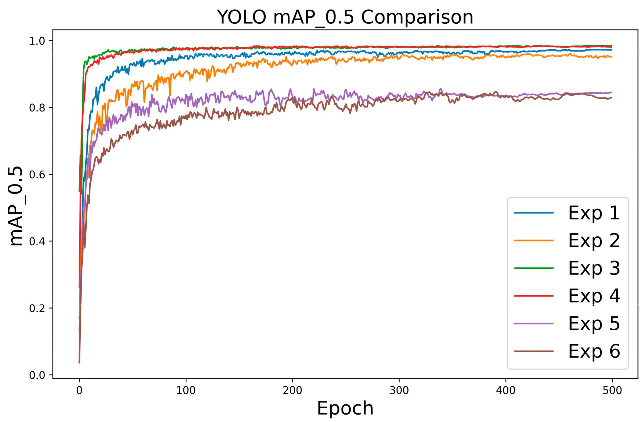
Regarding the parameter epoch, we first ran the six experiments (Table 3) with an epoch value of 500 and analyzed the mAP_0.5 values (Figure 9). In Figure 9, we can see that the mAP_0.5 values increased dramatically when the epoch value increased from 0 to 100, then stayed relatively stable when the epoch value increased from 100 to 200, and then remained the same when the epoch value was larger than 200. As a compromise of computation time and model accuracy, we selected the epoch value of 200 to evaluate the model performances in this study (Table 3).
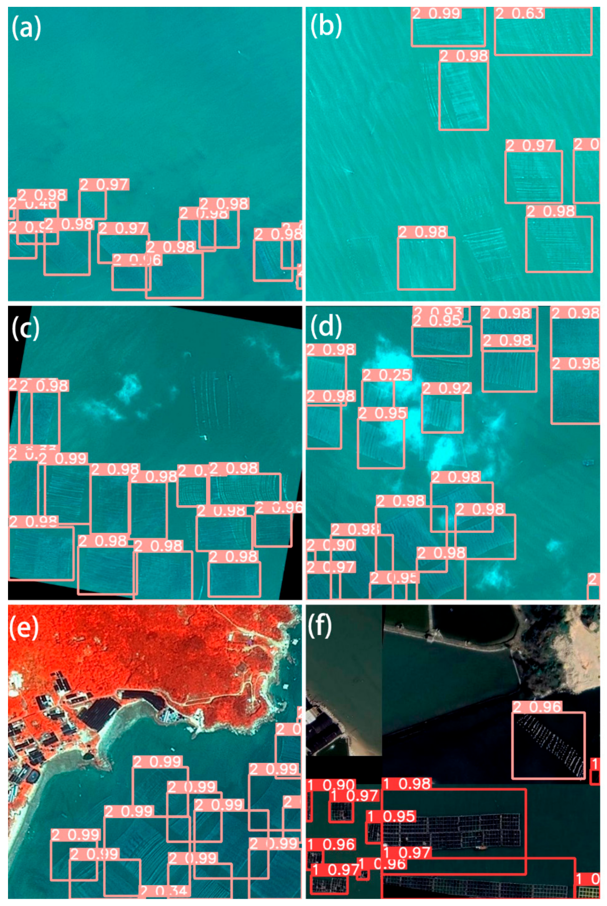
To make the models capable of detecting offshore aquaculture areas under different environmental conditions, we tried to collect as much sample data as possible. Figure 10a,b show the offshore aquaculture detection results derived from satellite imagery and the YOLOv5x model in calm water and turbulent water conditions. Figure 10c,d show the detection results under cloudy weather. Figure 10e,f show the detection results when islands or terrestrial land cover are present nearby. It can be seen that the YOLO models effectively detected offshore aquaculture areas in different sea states or when different land covers coexisted there. Furthermore, we found that the YOLO models could still detect the aquaculture areas when clouds partly obscured the features of the offshore aquaculture objects, demonstrating the robustness of the YOLO models for object detection.

5. Conclusions

The rapid and disordered expansion of artificial marine aquaculture makes it urgent and significant to accurately monitor offshore aquaculture areas. Although YOLO models have been widely used for marine object detection, they have not previously been employed for monitoring offshore aquaculture areas. This study therefore evaluated the capacity of two well-known YOLO models, YOLOv5 and YOLOv7, for offshore aquaculture detection based on different high-resolution optical remote sensing imagery. Based on the satellite dataset, YOLOv5 outperformed YOLOv7 in terms of Precision, Recall, F1 score, mAP_0.5, and average confidence values. Based on the Google Earth dataset, YOLOv5 and YOLOv7 showed similar results. The spatial resolution was an important factor that affected the YOLO models’ performance. Thus, we used the Real-ESRGAN method to enhance the spatial resolution of the satellite dataset and investigated whether SR methods could improve the detection accuracy of the YOLO models. The results indicated that despite improving the image clarity and resolution, SR methods can negatively affect the performance of YOLO models for offshore aquaculture object detection. So, attention should be paid to the use of SR methods before the application of deep learning models for object detection using high-spatial-resolution remote sensing imagery. Findings from this study are intended to contribute to the application of deep learning models for offshore aquaculture monitoring in the ocean.

Author Contributions

Conceptualization, D.D., H.H. and J.Y.; methodology, D.D., Q.S., P.H. and B.G.; software, Q.S. and P.H.; validation, D.D., Q.S., P.H., H.H., J.Y. and B.G.; formal analysis, Q.S., P.H. and Q.G.; investigation, D.D., Q.S., P.H., H.H., J.Y. and B.G.; resources, D.D.; data curation, Q.S. and P.H.; writing—original draft preparation, D.D., Q.S. and P.H.; writing—review and editing, D.D., H.H. and J.Y.; visualization, Q.S., P.H. and Q.G.; supervision, H.H. and J.Y.; project administration, H.H. and J.Y.; funding acquisition, H.H. All authors have read and agreed to the published version of the manuscript.

Funding

This work was funded by the Project Supported by the Director’s Foundation of South China Sea Bureau of Ministry of Natural Resources (230206); the Marine Economy Special Project of the Guangdong Province (GDNRC[2024]36). The APC was funded by the Science and Technology Project of Guangdong Forestry Administration (2024): Monitoring and Ecological Value Assessment of Coastal Wetland Resources in the Guangdong Province.

Data Availability Statement

The authors confirm that the data supporting the findings of this study are available within the article.

Acknowledgments

Thanks to the reviewers and editors for their valuable suggestions on this paper.

Conflicts of Interest

The authors declare no conflicts of interest.

References

  1. Fu, Y.; Deng, J.; Wang, H.; Comber, A.; Yang, W.; Wu, W.; You, S.; Lin, Y.; Wang, K. A new satellite-derived dataset for marine aquaculture areas in China’s coastal region. Earth Syst. Sci. Data 2021, 13, 1829–1842. [Google Scholar] [CrossRef]
  2. Rishikeshan, C.; Ramesh, H. An automated mathematical morphology driven algorithm for water body extraction from remotely sensed images. ISPRS-J. Photogramm. Remote Sens. 2018, 146, 11–21. [Google Scholar] [CrossRef]
  3. Hou, T.; Sun, W.; Chen, C.; Yang, G.; Meng, X.; Peng, J. Marine floating raft aquaculture extraction of hyperspectral remote sensing images based decision tree algorithm. Int. J. Appl. Earth Obs. Geoinf. 2022, 111, 102846. [Google Scholar] [CrossRef]
  4. Cao, L.; Wang, W.; Yang, Y.; Yang, C.; Yuan, Z.; Xiong, S.; Diana, J. Environmental impact of aquaculture and countermeasures to aquaculture pollution in China. Environ. Sci. Pollut. Res. 2007, 14, 452–462. [Google Scholar]
  5. Chen, C.; He, X.; Liu, Z.; Sun, W.; Dong, H.; Chu, Y. Analysis of regional economic development based on land use and land cover change information derived from Landsat imagery. Sci. Rep. 2020, 10, 12721. [Google Scholar] [CrossRef] [PubMed]
  6. Kang, J.; Sui, L.; Yang, X.; Liu, Y.; Wang, Z.; Wang, J.; Yang, F.; Liu, B.; Ma, Y. Sea surface-visible aquaculture spatial-temporal distribution remote sensing: A case study in Liaoning province, China from 2000 to 2018. Sustainability 2019, 11, 7186. [Google Scholar] [CrossRef]
  7. Cui, Y.; Zhang, X.; Jiang, N.; Dong, T.; Xie, T. Remote sensing identification of marine floating raft aquaculture area based on sentinel-2A and DEM data. Front. Mar. Sci. 2022, 9, 955858. [Google Scholar] [CrossRef]
  8. Zhou, W.; Wang, F.; Wang, X.; Tang, F.; Li, J. Evaluation of multi-source high-resolution remote sensing image fusion in aquaculture areas. Appl. Sci. 2022, 12, 1170. [Google Scholar] [CrossRef]
  9. Wen, Q.; Zhang, Z.; Xu, J.; Zuo, L.; Wang, X.; Liu, B.; Zhao, X.; Yi, L. Spatial and temporal change of wetlands in Bohai rim during 2000–2008: An analysis based on satellite images. J. Remote Sens. 2011, 15, 183–200. (In Chinese) [Google Scholar]
  10. Mialhe, F.; Gunnell, Y.; Mering, C. The impacts of shrimp farming on land use, employment and migration in Tumbes, northern Peru. Ocean Coast. Manag. 2013, 73, 1–12. [Google Scholar] [CrossRef]
  11. Tenório, G.S.; Souza-Filho, P.W.M.; Ramos, E.M.; Alves, P.J.O. Mangrove shrimp farm mapping and productivity on the Brazilian Amazon coast: Environmental and economic reasons for coastal conservation. Ocean Coast. Manag. 2015, 104, 65–77. [Google Scholar] [CrossRef]
  12. Rather, M.A.; Ahmad, I.; Shah, A.; Hajam, Y.A.; Amin, A.; Khursheed, S.; Ahmad, I.; Rasool, S. Exploring opportunities of Artificial Intelligence in aquaculture to meet increasing food demand. Food Chem. X 2024, 22, 101309. [Google Scholar] [CrossRef] [PubMed]
  13. Liu, Y.; Wang, Z.; Yang, X.; Zhang, Y.; Yang, F.; Liu, B.; Cai, P. Satellite-based monitoring and statistics for raft and cage aquaculture in China’s offshore waters. Int. J. Appl. Earth Obs. Geoinf. 2020, 91, 102118. [Google Scholar] [CrossRef]
  14. Zhou, C.; Wong, K.; Tsou, J.Y.; Zhang, Y. Detection and Statistics of Offshore Aquaculture Rafts in Coastal Waters. J. Mar. Sci. Eng. 2022, 10, 781. [Google Scholar] [CrossRef]
  15. Maxwell, A.E.; Warner, T.A.; Fang, F. Implementation of machine-learning classification in remote sensing: An applied review. Int. J. Remote Sens. 2018, 39, 2784–2817. [Google Scholar] [CrossRef]
  16. Wang, Z.; Yang, X.; Liu, Y.; Lu, C. Extraction of coastal raft cultivation area with heterogeneous water background by thresholding object-based visually salient NDVI from high spatial resolution imagery. Remote Sens. Lett. 2018, 9, 839–846. [Google Scholar] [CrossRef]
  17. Wang, S.; Huang, C.; Li, H.; Liu, Q. Synergistic Integration of Time Series Optical and SAR Satellite Data for Mariculture Extraction. Remote Sens. 2023, 15, 2243. [Google Scholar] [CrossRef]
  18. Wang, M.; Cui, Q.; Wang, J.; Ming, D.; Lv, G. Raft cultivation area extraction from high resolution remote sensing imagery by fusing multi-scale region-line primitive association features. ISPRS-J. Photogramm. Remote Sens. 2017, 123, 104–113. [Google Scholar] [CrossRef]
  19. LeCun, Y.; Bengio, Y.; Hinton, G. Deep learning. Nature 2015, 521, 436–444. [Google Scholar] [CrossRef] [PubMed]
  20. Chen, Y.; Wan, J.; Xi, Y.; Jiang, W.; Wang, M.; Kang, M. Extraction and Classification of the Supervised Coastal Objects Based on HSRIs and a Novel Lightweight Fully Connected Spatial Dropout Network. Wirel. Commun. Mob. Comput. 2022, 2022, 2054877. [Google Scholar] [CrossRef]
  21. Blaschke, T.; Hay, G.J.; Kelly, M.; Lang, S.; Hofmann, P.; Addink, E.; Feitosa, R.Q.; Van der Meer, F.; Van der Werff, H.; Van Coillie, F. Geographic object-based image analysis–towards a new paradigm. ISPRS-J. Photogramm. Remote Sens. 2014, 87, 180–191. [Google Scholar] [CrossRef] [PubMed]
  22. Chen, G.; Weng, Q.; Hay, G.J.; He, Y. Geographic object-based image analysis (GEOBIA): Emerging trends and future opportunities. GISci. Remote Sens. 2018, 55, 159–182. [Google Scholar] [CrossRef]
  23. Chen, J.; Lu, Y.; Yu, Q.T. Transformers make strong encoders for medical image segmentation. arXiv 2021, arXiv:2102.04306. [Google Scholar]
  24. Chen, Y.; He, G.; Yin, R.; Zheng, K.; Wang, G. Comparative study of marine ranching recognition in multi-temporal high-resolution remote sensing images based on DeepLab-v3+ and U-Net. Remote Sens. 2022, 14, 5654. [Google Scholar] [CrossRef]
  25. Deng, J.; Bai, Y.; Chen, Z.; Shen, T.; Li, C.; Yang, X. A Convolutional Neural Network for Coastal Aquaculture Extraction from High-Resolution Remote Sensing Imagery. Sustainability 2023, 15, 5332. [Google Scholar] [CrossRef]
  26. Pham, M.-T.; Courtrai, L.; Friguet, C.; Lefèvre, S.; Baussard, A. YOLO-Fine: One-stage detector of small objects under various backgrounds in remote sensing images. Remote Sens. 2020, 12, 2501. [Google Scholar] [CrossRef]
  27. Qu, P.; Cheng, E.; Chen, K. Real-Time Ocean Small Target Detection Based on Improved YOLOX Network. In Proceedings of the OCEANS 2022, Hampton Roads, VA, USA, 17–20 October 2022; pp. 1–5. [Google Scholar]
  28. Wang, S.; Gao, S.; Zhou, L.; Liu, R.; Zhang, H.; Liu, J.; Jia, Y.; Qian, J. YOLO-SD: Small ship detection in SAR images by multi-scale convolution and feature transformer module. Remote Sens. 2022, 14, 5268. [Google Scholar] [CrossRef]
  29. Ge, R.; Mao, Y.; Li, S.; Wei, H. Research On Ship Small Target Detection In SAR Image Based On Improved YOLO-v7. In Proceedings of the 2023 International Applied Computational Electromagnetics Society Symposium (ACES-China), Hangzhou, China, 15–18 August 2023; pp. 1–3. [Google Scholar]
  30. Wang, L.; Chen, L.-Z.; Peng, B.; Lin, Y.-T. Improved YOLOv5 Algorithm for Real-Time Prediction of Fish Yield in All Cage Schools. J. Mar. Sci. Eng. 2024, 12, 195. [Google Scholar] [CrossRef]
  31. Liu, H.; Ma, X.; Yu, Y.; Wang, L.; Hao, L. Application of deep learning-based object detection techniques in fish aquaculture: A review. J. Mar. Sci. Eng. 2023, 11, 867. [Google Scholar] [CrossRef]
  32. Zhou, S.; Cai, K.; Feng, Y.; Tang, X.; Pang, H.; He, J.; Shi, X. An accurate detection model of takifugu rubripes using an improved yolo-v7 network. J. Mar. Sci. Eng. 2023, 11, 1051. [Google Scholar] [CrossRef]
  33. Shi, Y.; Li, S.; Liu, Z.; Zhou, Z.; Zhou, X. MTP-YOLO: You Only Look Once Based Maritime Tiny Person Detector for Emergency Rescue. J. Mar. Sci. Eng. 2024, 12, 669. [Google Scholar] [CrossRef]
  34. Fang, Z.; Wang, X.; Zhang, L.; Jiang, B. YOLO-RSA: A Multiscale Ship Detection Algorithm Based on Optical Remote Sensing Image. J. Mar. Sci. Eng. 2024, 12, 603. [Google Scholar] [CrossRef]
  35. Yang, Z.; Yin, Y.; Jing, Q.; Shao, Z. A High-Precision Detection Model of Small Objects in Maritime UAV Perspective Based on Improved YOLOv5. J. Mar. Sci. Eng. 2023, 11, 1680. [Google Scholar] [CrossRef]
  36. Redmon, J.; Divvala, S.; Girshick, R.; Farhadi, A. You only look once: Unified, real-time object detection. In Proceedings of the IEEE Conference on Computer Vision and Pattern Recognition, Las Vegas, NV, USA, 27–30 June 2016; pp. 779–788. [Google Scholar]
  37. Redmon, J.; Farhadi, A. Yolov3: An incremental improvement. arXiv 2018, arXiv:1804.02767. [Google Scholar]
  38. Hong, Z.; Yang, T.; Tong, X.; Zhang, Y.; Jiang, S.; Zhou, R.; Han, Y.; Wang, J.; Yang, S.; Liu, S. Multi-scale ship detection from SAR and optical imagery via a more accurate YOLOv3. IEEE J. Sel. Top. Appl. Earth Observ. Remote Sens. 2021, 14, 6083–6101. [Google Scholar] [CrossRef]
  39. Hu, J.; Zhi, X.; Shi, T.; Zhang, W.; Cui, Y.; Zhao, S. PAG-YOLO: A portable attention-guided YOLO network for small ship detection. Remote Sens. 2021, 13, 3059. [Google Scholar] [CrossRef]
  40. Chen, Z.; Liu, C.; Filaretov, V.F.; Yukhimets, D.A. Multi-scale ship detection algorithm based on YOLOv7 for complex scene SAR images. Remote Sens. 2023, 15, 2071. [Google Scholar] [CrossRef]
  41. Du, S.; Huang, H.; He, F.; Luo, H.; Yin, Y.; Li, X.; Xie, L.; Guo, R.; Tang, S. Unsupervised stepwise extraction of offshore aquaculture ponds using super-resolution hyperspectral images. Int. J. Appl. Earth Obs. 2023, 119, 103326. [Google Scholar] [CrossRef]
  42. Gu, Y.-G.; Lin, Q. Trace metals in a sediment core from the largest mariculture base of the eastern Guangdong coast, South China: Vertical distribution, speciation, and biological risk. Mar. Pollut. Bull. 2016, 113, 520–525. [Google Scholar] [CrossRef] [PubMed]
  43. Gu, Y.-G.; Gao, Y.-P.; Jiang, S.-J.; Jordan, R.W.; Yang, Y.-F. Ecotoxicological risk of antibiotics and their mixtures to aquatic biota with the DGT technique in sediments. Ecotoxicology 2023, 32, 536–543. [Google Scholar] [CrossRef] [PubMed]
  44. Gu, Y.-G.; Lin, Q.; Jiang, S.-J.; Wang, Z.-H. Metal pollution status in Zhelin Bay surface sediments inferred from a sequential extraction technique, South China Sea. Mar. Pollut. Bull. 2014, 81, 256–261. [Google Scholar] [CrossRef]
  45. Gu, Y.-G.; Ouyang, J.; Ning, J.-J.; Wang, Z.-H. Distribution and sources of organic carbon, nitrogen and their isotopes in surface sediments from the largest mariculture zone of the eastern Guangdong coast, South China. Mar. Pollut. Bull. 2017, 120, 286–291. [Google Scholar] [CrossRef]
  46. Gu, Y.-G.; Ke, C.-L.; Liu, Q. Characterization, sources, and ecological hazards of polycyclic aromatic hydrocarbons in the intertidal sediments of Zhelin Bay, the biggest mariculture area on the eastern Guangdong coast of China. Mar. Pollut. Bull. 2018, 130, 192–197. [Google Scholar] [CrossRef]
  47. Yue, L.; Shen, H.; Li, J.; Yuan, Q.; Zhang, H.; Zhang, L. Image super-resolution: The techniques, applications, and future. Signal Process. 2016, 128, 389–408. [Google Scholar] [CrossRef]
  48. Wang, X.; Yu, K.; Wu, S.; Gu, J.; Liu, Y.; Dong, C.; Qiao, Y.; Change Loy, C. Esrgan: Enhanced super-resolution generative adversarial networks. In Proceedings of the European Conference on Computer Vision (ECCV) Workshops, Munich, Germany, 8–14 September 2018; pp. 63–79. [Google Scholar]
  49. Wang, P.; Bayram, B.; Sertel, E. A comprehensive review on deep learning based remote sensing image super-resolution methods. Earth-Sci. Rev. 2022, 232, 104110. [Google Scholar] [CrossRef]
  50. Wang, Y.; Sun, G.; Guo, S. Target detection method for low-resolution remote sensing image based on esrgan and redet. Photonics 2021, 8, 431. [Google Scholar] [CrossRef]
  51. Wang, X.; Xie, L.; Dong, C.; Shan, Y. Real-esrgan: Training real-world blind super-resolution with pure synthetic data. In Proceedings of the IEEE/CVF International Conference on Computer Vision, Montreal, BC, Canada, 11–17 October 2021; pp. 1905–1914. [Google Scholar]
  52. Real-ESRGAN. Available online: https://github.com/xinntao/Real-ESRGAN (accessed on 16 April 2024).
  53. Shorten, C.; Khoshgoftaar, T.M. A survey on image data augmentation for deep learning. J. Big Data 2019, 6, 60. [Google Scholar] [CrossRef]
  54. Tao, J.; Wang, H.; Zhang, X.; Li, X.; Yang, H. An object detection system based on YOLO in traffic scene. In Proceedings of the 2017 6th International Conference on Computer Science and Network Technology (ICCSNT), Dalian, China, 21–22 October 2017; pp. 315–319. [Google Scholar]
  55. Ma, R.; Zhang, R. Facial expression recognition method based on PSA—YOLO network. Front. Neurorobot. 2023, 16, 1057983. [Google Scholar] [CrossRef] [PubMed]
  56. Abdullah; Ali, S.; Khan, Z.; Hussain, A.; Athar, A.; Kim, H.-C. Computer vision based deep learning approach for the detection and classification of algae species using microscopic images. Water 2022, 14, 2219. [Google Scholar] [CrossRef]
  57. Durve, M.; Orsini, S.; Tiribocchi, A.; Montessori, A.; Tucny, J.-M.; Lauricella, M.; Camposeo, A.; Pisignano, D.; Succi, S. Benchmarking YOLOv5 and YOLOv7 models with DeepSORT for droplet tracking applications. Eur. Phys. J. E 2023, 46, 32. [Google Scholar] [CrossRef] [PubMed]
  58. Hussain, M. YOLO-v1 to YOLO-v8, the rise of YOLO and its complementary nature toward digital manufacturing and industrial defect detection. Machines 2023, 11, 677. [Google Scholar] [CrossRef]
  59. Wu, D.; Jiang, S.; Zhao, E.; Liu, Y.; Zhu, H.; Wang, W.; Wang, R. Detection of Camellia oleifera fruit in complex scenes by using YOLOv7 and data augmentation. Appl. Sci. 2022, 12, 11318. [Google Scholar] [CrossRef]
  60. Jocher, G.; Nishimura, K.; Mineeva, T.; Vilariño, R. YOLOv5 (2020). GitHub Repository. Available online: https://github.com/ultralytics/yolov5 (accessed on 1 December 2023).
  61. Jocher, G.; Chaurasia, A.; Stoken, A.; Borovec, J.; Kwon, Y.; Michael, K.; Fang, J.; Wong, C.; Yifu, Z.; Montes, D. ultralytics/yolov5: v6. 2-yolov5 classification models, apple m1, reproducibility, clearml and deci. ai integrations. Zenodo 2022. [Google Scholar] [CrossRef]
  62. YOLOv7. Available online: https://github.com/WongKinYiu/yolov7 (accessed on 16 April 2024).
  63. Kee, E.; Chong, J.J.; Choong, Z.J.; Lau, M. A comparative analysis of cross-validation techniques for a smart and lean pick-and-place solution with deep learning. Electronics 2023, 12, 2371. [Google Scholar] [CrossRef]
  64. Arani, E.; Gowda, S.; Mukherjee, R.; Magdy, O.; Kathiresan, S.; Zonooz, B. A comprehensive study of real-time object detection networks across multiple domains: A survey. arXiv 2022, arXiv:2208.10895. [Google Scholar]
  65. Olorunshola, O.E.; Irhebhude, M.E.; Evwiekpaefe, A.E. A comparative study of YOLOv5 and YOLOv7 object detection algorithms. J. Comput. Soc. Inf. 2023, 2, 1–12. [Google Scholar] [CrossRef]
  66. Salman, S.; Liu, X. Overfitting mechanism and avoidance in deep neural networks. arXiv 2019, arXiv:1901.06566. [Google Scholar]
  67. Ying, X. An overview of overfitting and its solutions. J. Phys. Conf. Ser. 2019, 1168, 022022. [Google Scholar]
  68. Bejani, M.M.; Ghatee, M. A systematic review on overfitting control in shallow and deep neural networks. Artif. Intell. Rev. 2021, 54, 6391–6438. [Google Scholar] [CrossRef]
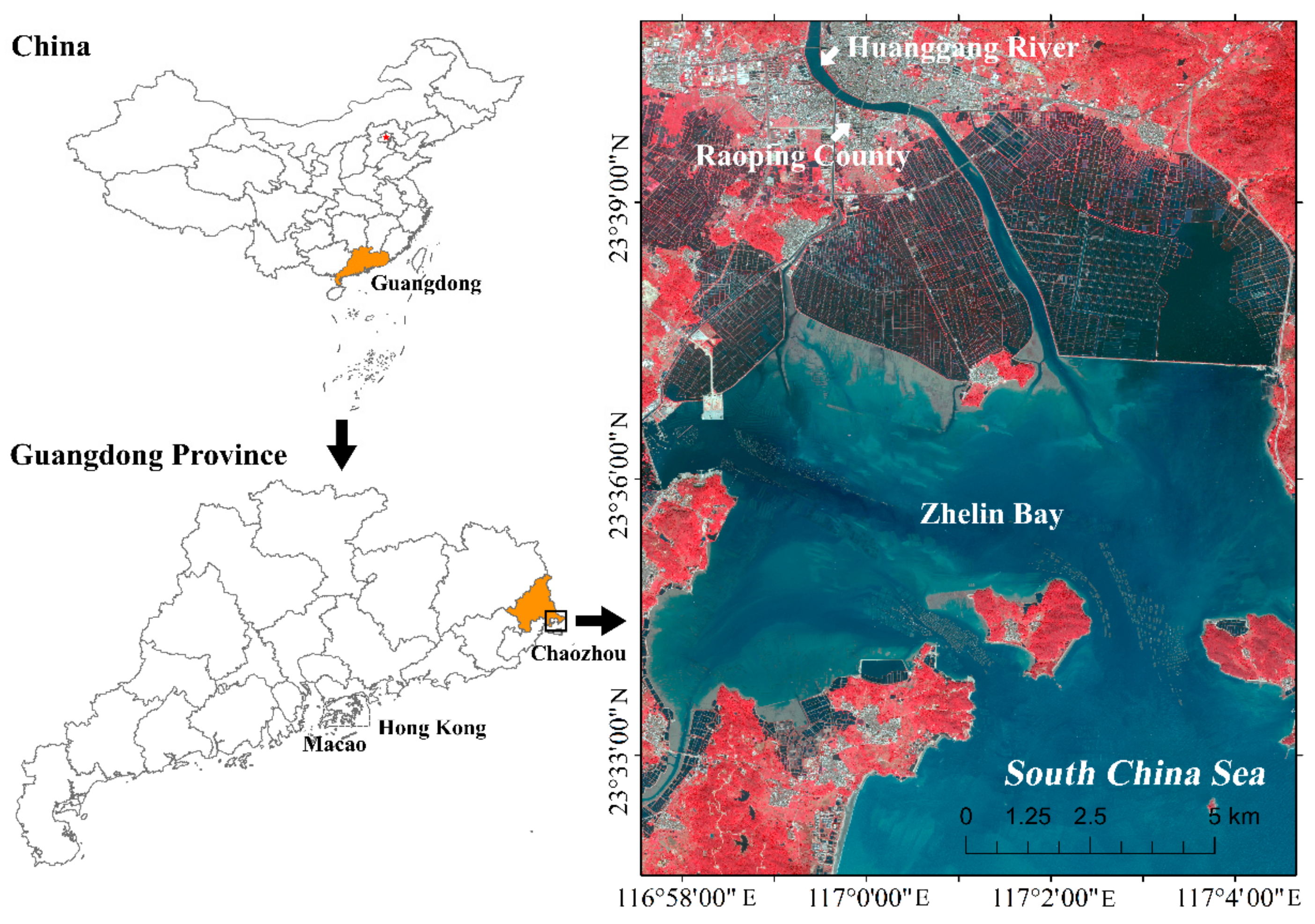
Figure 1. Map showing the location of Zhelin Bay in Guangdong Province. The image on the right shows Zhelin Bay in the form of standard false-color Gaofen-1B image.
Jmse 12 01012 g001
Figure 2. Different offshore aquaculture types on Google Earth imagery.
Jmse 12 01012 g002
Figure 3. Different offshore aquaculture types in the satellite imagery.
Jmse 12 01012 g003
Figure 4. Different offshore aquaculture types in SR-augmented satellite imagery.
Jmse 12 01012 g004
Figure 5. Augmented sample images.
Jmse 12 01012 g005
Figure 6. YOLOv5 network architecture.
Jmse 12 01012 g006
Figure 7. YOLOv7 network architecture.
Jmse 12 01012 g007
Figure 8. Object detection results using YOLOv5 and YOLOv7 algorithms based on satellite and Google Earth (GE) datasets.
Jmse 12 01012 g008
Figure 9. The mAP_0.5 curves of Experiment 1–Experiment 6 when the epoch value was 500.
Jmse 12 01012 g009
Figure 10. The offshore aquaculture detection results using the YOLOv5x model in calm water (a) and turbulent water conditions (b), under cloudy weather (c,d), and when islands or terrestrial land cover existed nearby (e,f).
Jmse 12 01012 g010
Table 1. Key parameters of satellite camera systems.
PlatformSensorBand NumberSpectral Range/μmSpatial Resolution/mPlatformSensorBand NumberSpectral Range/μmSpatial Resolution/m
-0.45–0.902ZY3-02Front camera-0.50–0.802.5
Gaofen-1BPAN *
MS *
10.45–0.528Rear camera-0.50–0.802.5
20.52–0.59Nadir camera-0.50–0.802.1
30.63–0.69MS10.45–0.525.8
40.77–0.8920.52–0.59
Gaofen-6PAN-0.45–0.902 30.63–0.69
MS10.45–0.52840.77–0.89
20.52–0.60
30.63–0.69
40.76–0.90
* PAN refers to a camera operating on the panchromatic band, and MS refers to a camera operating on multispectral bands.
Table 2. Experimental environment.
ProjectModel/Parameter
CPUIntel Core 2 Duo T7700
RAM32 GB
GPUNVIDIA GRID RTX8000-48Q
SystemWindows 10
CodePython3.7
FrameworkCUDA11.0/cudnn8.0.1/torch 1.7.1
Table 3. The detection results of YOLOv5 and YOLOv7.
Experiment IDModelData SetPrecision (%)Recall (%)F1 ScoremAP_0.5 (%)Frames per Second (FPS)
1YOLOv5Satellite95.3393.0294.1696.2232.89
2YOLOv7Satellite92.0490.9991.5194.1932.05
3YOLOv5Google Earth96.6795.9196.2998.233.22
4YOLOv7Google Earth96.2795.8196.0498.1633.33
5YOLOv5Satellite (SR) *86.280.2883.1385.533.22
6YOLOv7Satellite (SR) *75.8479.3177.5481.3332.36
* Satellite (SR) denotes the SR-augmented satellite dataset.
Table 4. The p-values of different models.
Data SetModelPrecisionRecallF1 ScoremAP_0.5Frame per Second
Google EarthYOLOv5 vs. YOLOv70.300.680.0890.520.71
SatelliteYOLOv5 vs. YOLOv7* 0.021* 0.024* 0.0025* 6.49 × 10−50.13
Satellite (SR)YOLOv5 vs. YOLOv7* 2.42 × 10−50.33* 1.16 × 10−7* 3.53 × 10−40.58
* denotes significant difference according to the paired t-test at the 5% significance level.
Table 5. The p-values of different datasets.
ModelData SetPrecisionRecallF1 ScoremAP_0.5Frame per Second
YOLOv5Google Earth vs. Satellite0.27* 0.0039* 0.027* 9.16 × 10−40.11
Satellite vs. Satellite (SR)* 5.72 × 10−5* 1.83 × 10−6* 6.87 × 10−7* 1.78 × 10−7* 0.0096
YOLOv7Google Earth vs. Satellite* 2.60 × 10−5* 4.72 × 10−4* 1.26 × 10−5* 6.96 × 10−50.032
Satellite vs. Satellite (SR)* 1.07 × 10−5* 5.28 × 10−6* 1.81 × 10−7* 1.63 × 10−60.78
* denotes significant difference according to the paired t-test at the 5% significance level.
Table 6. Average confidence values of different models and different datasets.
ModelData SetAverage Confidence
YOLOv5Satellite0.90
YOLOv7Satellite0.86
YOLOv5Google Earth0.85
YOLOv7Google Earth0.81
Table 7. Average confidence values of different models and datasets using different confidence thresholds.
Conf_thresYOLOv5 + SatelliteYOLOv7 + SatelliteYOLOv5 + Google EarthYOLOV7 + Google Earth
0.30.910.870.870.83
0.40.920.880.890.85
0.50.920.890.900.87
0.60.930.900.910.89
0.70.930.910.930.91
0.80.940.930.940.92
0.90.960.950.960.95
Disclaimer/Publisher’s Note: The statements, opinions and data contained in all publications are solely those of the individual author(s) and contributor(s) and not of MDPI and/or the editor(s). MDPI and/or the editor(s) disclaim responsibility for any injury to people or property resulting from any ideas, methods, instructions or products referred to in the content.