Abstract
Unmanned sailboats, harnessing wind for propulsion, offer great potential for extended marine research due to their virtually unlimited endurance. The sails typically operate at high attack angles, which contrasts with aircraft that maintain small angles to prevent stalling. Despite the reduction in lift during stalling, the resultant increase in drag contributes significantly to the sail’s thrust. However, the sail often experiences vortex shedding due to high attack angles, leading to low-frequency oscillations and erratic navigation. This study employs large-eddy simulations (LESs) on a 3D NACA0012 sail at a Reynolds number of 3.6 × 10⁵, which is validated by experimental data. It observes the lift and drag coefficients across attack angles from 5 to 90 degrees and compares these with a Dynarig sail. The findings reveal that higher attack angles amplify fluctuations in lift and drag coefficients. Vortex shedding, resulting from flow separation, creates pressure changes and oscillations in aerodynamic forces. Fast Fourier transformation (FFT) analysis identifies dominant frequencies between 0.5 and 10 Hz, indicating low-frequency oscillations. The study’s insights into the impact of attack angle and sail type on the oscillation frequency are favorable for the design of unmanned sailboats, aiding in the prediction of wind-induced frequencies and optimal attack angle determination.
1. Introduction
Unmanned sailboats have the ability to continuously undertake marine hydrometeorological investigations on open seas. Harvesting wind energy as the main thrust power makes them stand out from other long-range and long-duration survey equipment [1]. In the next decade, unmanned sailboats are likely to become a potential solution for existing problems such as underwater communication [2].
Most unmanned sailboats from industry apply rigid wing sails as a propelling component [3]. Rigid sails allow unmanned sailboats to navigate with increased performance due to less power consumption and mechanically simpler control, which have increased robustness compared to traditional soft sails [4]. The sail size of major unmanned sailboats is mostly 1–10 m, which makes for a Reynolds number regime of 5.0 × 10⁴ to 5.0 × 10⁵. This is considered a low Reynolds number regime, where the viscosity will make a difference.
Ignoring the influence of low Reynolds numbers is one of the primary reasons that wing sails, despite being more efficient than traditional soft sails, have not achieved a breakthrough [5]. At low Reynolds numbers, the laminar boundary layer is more prone to separation compared to high Reynolds numbers. In other words, the boundary layer cannot sustain itself and physically detaches from the wing sail surface. After separation, the flow becomes unstable and transitions into turbulence. Under certain conditions, this airflow can reattach to the wing sail, forming a recirculation region known as a laminar separation bubble [6,7]. As the angle of attack of the sail increases, the shedding of vortices and/or the flapping of shear layers can easily induce low-frequency flow oscillations or even irregular fluctuations. This phenomenon leads to oscillations in the thrust exerted by the sail, posing a threat to propulsion stability. The periodic or quasi-periodic aerodynamic forces acting on the sail result in torque variations, causing unpredictable behavior during the navigation of unmanned sailboats. If the oscillation frequency is comparable to the roll, heave, or pitch motions of the sailboat, it may lead to fluctuations in the external forces acting on the sailboat, potentially causing resonance or even the risk of capsizing. Therefore, it is necessary to conduct in-depth research on wind-induced low-frequency oscillations (LFOs).
The state of LFOs is akin to the condition of a wing nearing or reaching stall. In a study by Almutairi [8], oscillations are considered self-sustaining, induced by the periodic formation and bursting of bubbles on the wing’s suction surface. The backflow within the bubbles indicates an absolutely unstable mechanism, with the trailing edge playing a significant role in driving the reattachment of the separated flow. Eljack et al. [9,10] conducted large-eddy simulations on an NACA0012 airfoil at a Reynolds number of 5.0 × 10⁴. The fundamental mechanism of low-frequency oscillation is described as a “button whirligig.” As the oscillatory flow loses momentum, the vortex triangle reverses the rotational direction of the flow, imparting an energy pulse that causes it to rotate counterclockwise, initiating a new imbalance. Ultimately, the instantaneous flow field switches between the attachment and separation phases in a periodic manner, with some disturbed cycles. Elawad et al. [11] performed large-eddy simulations on an NACA0012 airfoil at a Reynolds number of 9.0 × 10⁴. They demonstrated that laminar separation bubbles form on the suction surface, which are unstable and oscillate between short and open bubbles. The instability of the laminar separation bubbles leads to low-frequency flow oscillations.
Computational fluid dynamics (CFD) is a commonly employed method for studying the flow field around sails capable of obtaining detailed flow parameters at a relatively low cost, yet it has non-negligible limitations in precision. Previous aerodynamic studies of sails have largely focused on the time-averaged flow field. However, research by Arredondo et al. [12] revealed that the flow state on the suction side of the sail is intermittently attached, necessitating the use of transient solutions and corresponding turbulence models, rather than simulations based on time-averaging. William et al. [13] and Cravero [14] employed large-eddy simulation (LES) and detached-eddy simulation (DES) techniques, respectively, to assess vortex shedding on airfoils, achieving better flow field results than those based on time-averaged simulations. Zhu et al. [15] used an improved delayed detached-eddy simulation (IDDES) and observed more complex vortex shedding phenomena, revealing high-frequency and wake characteristics of the flow field, which displayed the high-frequency features of the external loads more effectively than unsteady Reynolds-averaged Navier–Stokes (URANS) simulations. Therefore, to better capture transient features of the flow field such as vortex shedding, higher-precision fluid simulation models like DES or LES should be adopted. Moreover, methods such as direct noise computation (DNC) and direct numerical simulation (DNS) can provide more detailed information on the flow field. Dawi et al. [16] utilized DNC to compute the flow past the vehicle mode at low Mach numbers. Akkermans et al. [17] presented an application of a computational aeroacoustics code as a hybrid zonal DNS tool, which showed good application for a 2D circular cylinder and a 3D decaying flow. DNC and DNS methods provide a more direct approach to flow computation, but are more computationally intensive, while LES offers a balance between accuracy and computational cost by focusing on the large-scale structures in turbulent flows. Therefore, the LES method is selected as the main tool to generate the data in this study.
The characteristics of low-frequency oscillations can be studied through spectral analysis [18], which identifies the frequency of each significant element within a data segment. Jabbari et al. [19] investigated the aerodynamic properties and ground effects of the NASA LS (1)-0417 airfoil at a Reynolds number of 1.69 × 10⁵, applying Fourier transform for frequency analysis. This revealed variations in the mean vorticity distribution and power spectral density relative to the Strouhal number (St). In most cases, a dominant frequency can be extracted from the LFO. Eljack et al. [20] discussed the flow oscillations of the NACA0012 airfoil at Reynolds numbers of 5.0 × 10⁴ and 9.0 × 10⁴. Spectral analysis of the lift coefficient at angles of attack of α = 9.25–10.5° indicated that both the Reynolds number and angle of attack are significant factors affecting the oscillation frequency. At higher Reynolds numbers, the spectrum does not show low-frequency peaks when the angle of attack is below or equal to the stall angle. They calculated St for different angles of attack, and found a local minimum near the stall angle. Moise et al. [21] discovered through simulation calculations and spectral analysis that at a free-stream Reynolds number of 5.0 × 10⁴, the NACA0012 airfoil exhibits low-frequency self-sustained oscillations at St ≈ 0.06 under zero incidence.
Sailing vessels typically operate at high attack angles, which contrasts with aircraft that maintain small angles to prevent stalling. From the perspective of thrust, both lift and drag on the sails can be considered contributors. Particularly in downwind conditions, to increase the speed of the vessel, larger angles of attack (typically exceeding 20°) are preferred. In these cases, the sails are in a fully stalled state, with fully developed turbulence in the wake. However, there is a lack of systematic research on LFOs at low Reynolds numbers and high angles of attack.
In this research, large-eddy simulations are performed on a 3D NACA0012 sail at a Reynolds number of 3.6 × 10⁵, facilitating the analysis and virtual representation of flow characteristics. The range of angles of attack was established from 5° to 90°. Spectral analysis was employed to investigate the frequency or Strouhal number distribution adjacent to the angle of attack. Further computational simulations and analyses of a Dynarig arc-shaped sail were conducted and compared with the spectral analysis results of the NACA0012 sail, yielding the distribution of low-frequency oscillations of the sail at various angles of attack.
It is noteworthy that LFOs have many potential influencing factors, such as the waves and the existence of the hull. A comprehensive study of all LFO factors would undoubtedly aid in revealing the true mechanisms of the interaction. However, the strong coupling between these factors hinders the provision of a final solution. This research will focus on the effects of attack angle on two sail types. Other influencing factors would be subject to future research.
This study is an expansion of our previous conference presentation [18]. The current work includes extensive new research findings from an additional sail geometry, the Dynarig sail. Further conclusions have been drawn regarding the influence of sail type on the shape and frequency of vortices in the wake. These represent a substantial advancement beyond the preliminary results and discussions outlined in the initial work.
In Part 2, the mathematical modeling, geometric model, numerical setting, and basic information of the fast Fourier transform are introduced. Part 3 is dedicated to the verification and validation of the computational code. Part 4 delineates the outcomes and deliberations pertaining to the sail thrust performance and spectral analysis. Finally, Part 5 articulates the conclusions of the study.
2. Methods
In this part, the mathematical modeling, geometric model of the simulations, and numerical setup will be introduced in sequence.
2.1. Mathematical Modeling
2.1.1. Governing Equations
In the present study, the flow is governed by the viscous incompressible Navier–Stokes equations. The momentum equation is shown as follows:
where u is the flow velocity, ∇ is the divergence, t is time, ν is the kinematic viscosity, p is the pressure, and f represents body force.
LES is applied to deal with turbulence by which the large scales of the turbulence are directly resolved everywhere in the flow domain, and the small-scale motions are modeled. The LES equations are shown as follows:
where and are the filtered velocities and is the filtered pressure. In turbulent flows, the forces due to pressure and viscous stresses are typically much larger than body forces f like gravity. Therefore, the latter can be neglected without significantly affecting the accuracy of the simulation. is the residual stress tensor, which can be calculated through the following equation [22]:
2.1.2. Lambda2 Criterion
The lambda2 criterion is a vortex core line detection algorithm that can adequately identify vortices from a three-dimensional fluid velocity field. Lambda2 is defined by the second-largest eigenvalue of S2 + Ω2. S and Ω are defined as follows:
where S is the strain-rate tensor and Ω is the spin tensor, which are the symmetric and antisymmetric parts of the velocity gradient J, respectively. Negative values of lambda2 can be interpreted as vortex regions, while values equal to or greater than 0 have no physical interpretation. In the present study, this scalar is applied to show the vortices’ development in the flow field.
2.2. Geometric Model
The computational domain is determined in Figure 1, and consists of a half cylinder and a box. The chord of the sail is c, Dx is 6c, Dz is c (Dz is 1/3c for Dynarig cases), and the radius R is 5c.
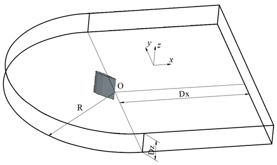
Figure 1.
The size of the computational domain.
A Cartesian coordinate system is defined, as shown in Figure 2. On the x-o-y plane, the center of the sail Ce locates at (−c/2, 0). The sail rotates clockwise by 45 degrees based on the vertical axis through Ce. Figure 2 presents the NACA0012 [23] sail as a representative, and the Dynarig sail has a similar definition. The symbol α is the attack angle.
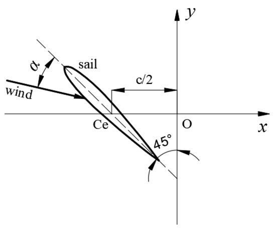
Figure 2.
The coordinate system and sail position.
The coefficient of lift (CL) and the coefficient of drag (CD) are defined as follows:
where L is the lift, D is the drag, ρ here represents the air density, V is the apparent flow speed, and S is the surface area of the sail.
In the present study, the position of the sail remains fixed and the attack angle is controlled by altering the direction of the incoming flow. Forces in x and y directions, Fx and Fy, can be exported directly through simulations, and L and D can thus be achieved through:
During the calculations, a Reynolds number of 3.6 × 10⁵ is selected to simulate the reality of a typical unmanned sailboat. It is also in accordance with the available experimental data for the NACA0012 sail. The Reynolds number Re is defined as follows:
where V is the apparent flow speed, c is the chord of the sail, and ν is the kinematic viscosity.
2.3. Numerical Setting
2.3.1. Solver and Mesh
Simulations in the present study are performed in a commercial solver Star-CCM+ (v16.02). Unsteady incompressible Navier–Stokes equations together with the LES model are used to resolve the flow domain. The bounded central scheme is applied to the convection equations in a segregated flow solver. The WALE (wall-adapting local-eddy viscosity) model is selected as the subgrid-scale model.
The trimmed cell mesher and the prism layer mesher are applied to generate the mesh. The prism layer contains 26 layers of cells, and the adjacent layers have a stretch ratio of 1.15. The nondimensional thickness of the first prism layer y+ is less than one. All y+ wall treatment is implemented in the wall-bounded flow during calculations.
Mesh cells close to the sails are refined by controlling the cell size in a refinement circle around the sail. The chord length and initial velocity for both sails are listed in Table 1. Since the LES model is designed to simulate more vortex details in flow, the mesh in the wake is refined accordingly. A close-up of the computational grid near the NACA0012 sail is shown in Figure 3.

Table 1.
Basic parameters for NACA0012 and Dynarig sails.
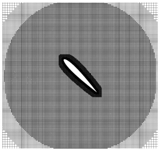
Figure 3.
A close-up of the grid around the sail (Darker areas identify denser grids).
The condition Courant number < 1 is ensured throughout the computation domain. All simulations were performed on a 6-node cluster with 48 CPUs on each node. One full node was used for a single simulating case. Four full days (the physical time is about five seconds) were needed to converge. In determining the convergence of the computation, two conditions must be satisfied: firstly, all residuals must decrease by more than three orders of magnitude; secondly, the monitored values of lift and drag must either stabilize or exhibit periodic variation as the computation progresses. When both of these conditions are met concurrently, it can be concluded that the computation has reached a state of convergence.
2.3.2. Boundary Conditions
The boundary conditions set in this study are illustrated in Figure 4. The arc boundary surface on the left side is set as velocity inlet. The range of the incoming flow is +45° to −45°. The two side boundaries are set as velocity inlet or pressure outlet, which is determined based on the wind direction. The sail is fixed in the domain and its surface is set to a no-slip wall. The right boundary is set as a pressure outlet, where the boundary physical values are extrapolated from the interior of the solution domain. The reference pressure is set to zero.
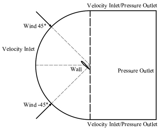
Figure 4.
The computational domain and boundary conditions.
The boundary condition of the surfaces parallel to the paper are set as symmetry. The limitation is that the calculations will lose the physical details near the wingtip, but this setting is in accordance with the wind tunnel test. The vortices generated by the wingtip will be looked into in a future study.
2.4. Fast Fourier Transform (FFT)
CL and CD can be exported from the simulations explicitly in the time domain. It can be observed that for large attack angles, low-frequency or irregular oscillations occur, which can be considered a superposition of many regular waves. This study will apply Fourier transform to analyze oscillations in the frequency domain.
In the present study, the sampling interval is 10,000 Hz (1 × 10⁻⁴ s), and thus discrete Fourier transform (DFT) can be applied to achieve the frequency distribution. The DFT is defined by the formula:
where k = 0, 1, 2, …, N − 1. Fast Fourier transform (FFT) is a fast-computing algorithm of DFT. It is obtained by improving the algorithm of DFT according to its odd–even characteristics, which can reduce the computations from the magnitude N2 to NlogN. This characteristic will dramatically save time spent on data analysis in this study.
3. Verification and Validation
In this part, the way to conduct computing verification is discussed, together with the exploration of several numerical settings on the results. The results of LESs are further validated with experiments to evaluate the accuracy of the code.
3.1. Verification
Four grids are generated for each sail to evaluate the mesh dependency, with a factor k = 1.2. The factor k means the number of mesh points in x, y, and z directions are 1.2 times more than the adjacent coarse mesh. The value of the initial y+ is set as a constant (y+ = 0.9) for all grids, since it is expected that the code can solve the flow parameters in the boundary layer directly. The influence of the y+ on the calculations can be found in Zeng et al. [24], which is not within the scope of this study. The cell numbers and results for the NACA0012 sail and the Dynarig sail are shown in Table 2.
Table 2.
Grid information and results for two sail types.
The evaluation method for discretization errors and uncertainties can refer to some previous studies [25,26], and the corresponding equations are omitted here. The uncertainties are computed for the densest grid, and the results are shown in Table 3.
Table 3.
Grid discretization errors and uncertainties.
Based on Table 3, the uncertainties for both sail types are in the range of 5–7%, which should be kept in mind for applications. Therefore, the final numbers of cells for the NACA0012 sail and Dynarig sail are about 14 million and 11 million, respectively.
Furthermore, to assess the impact of the number of cell layers in the boundary on the results, this study conducted simulations using three different layer counts based on the NACA0012 airfoil profile, with the results presented in Table 4.
Table 4.
Influence of the number of boundary layers on CL and CD.
The error between each adjacent case is less than 1%, indicating that the number of cell layers in the boundary has little influence on the results and can be neglected. In this study, 26 layers in the boundary are applied for all cases.
3.2. Validation
Wind tunnel tests performed by Sheldahl et al. [27] are applied to validate the CFD calculations. In their experiments, an NACA0012 airfoil was used, and the Reynolds number was 3.6 × 10⁵, which is in line with this study. Comparisons of the time-averaged lift and drag coefficients between the experimental results and LES computations are shown in Figure 5. The angle of attack varied from 5 to 90 degrees.
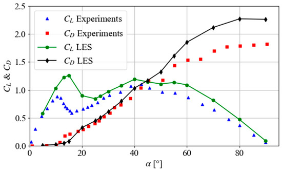
Figure 5.
Validation of the averaged lift and drag coefficients (Re = 3.6 × 10⁵, NACA0012).
For the attack angle α < 10°, CL and CD agree well with the experimental results (error < 10%). However, in the range of 10–20°, values of CL derived by LES are more than 50% higher and values of CD are 50% less than those in experiments. This phenomenon may be due to the fact that the applied numerical model is not adept at capturing the transition from attached flow to separated flow. For 20° < α ≤ 45°, both CL and CD have good agreement with the tests (less than 5%). For higher attack angles (>45 degrees), errors of CL and CD are 10–25%. The aforementioned error characteristics should be taken into consideration in the practical application of numerical results.
Localized disagreement in certain areas might be due to discordance in the initial conditions between simulations and experiments, such as the turbulence intensity (which will be further discussed later), the precision of the measurement equipment in the tests, or other numerical settings. Although these localized errors exist, the LES can capture the trend and features of the values of both CL and CD.
As one of the initial conditions, turbulence intensity may affect the final results of force coefficients. In this section, three values of turbulence of intensity, i.e., 0.1%, 1.0%, and 2.5%, are applied to evaluate their influence on CL and CD, which is shown in Figure 6. In this case, the attack angle is 30 degrees and the Reynolds number is 3.6 × 10⁵. To make an explicit comparison with experiments, the corresponding values of CL and CD in the tunnel test are also shown in this figure.
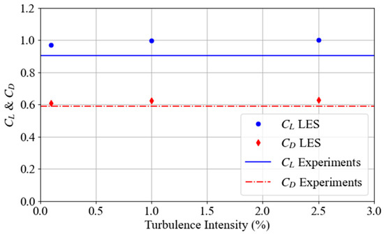
Figure 6.
Lift and drag coefficients against the turbulence intensity (the attack angle is 30 degrees).
The results presented in Figure 6 indicate that CL and CD are not significantly affected by turbulence intensity (less than 3% difference). Furthermore, it appears that lower turbulence intensity leads to smaller values of CL and CD. Therefore, the initial level of turbulence in the incoming flow has a negligible effect on the computation of forces acting on the sail.
In summary, from the perspectives of both verification and validation, the results obtained through numerical computation are deemed reliable. The numerical configuration employed will be consistently applied in the subsequent sections.
4. Results and Analysis
In this section, the lift and drag coefficients derived by LES computations are presented for different attack angles. Comparisons of flow field are made between the NACA0012 sail and Dynarig sail, and spectrum analysis is applied to evaluate the dominant frequency of the oscillations.
4.1. Force Performance of NACA0012 Sail
Computational results of lift and drag in the time domain are recorded in the simulations. Four angles of attack, i.e., α = 15°, 30°, 45°, and 90°, are selected as representatives, and the corresponding results of CL and CD are shown in Figure 7. In this figure, values of CL are displayed for α = 15°, 30° and 45°. Values of CD are shown for α = 90°, since the corresponding values of CL are small and do not contain useful information. The abscissa axis is nondimensionalized by tU0/c, where t is the physical time and U0 is the velocity of the incoming flow.
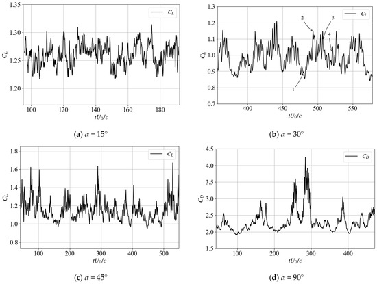
Figure 7.
Nondimensional time history for lift or drag coefficient for different angles of attack (annotations from 1 to 4 in (b) are illustrated in Figure 8).
Based on Figure 7, it can be seen that:
- When α = 15°, wiggles in CL are generally located in a small range of 1.225–1.300. Since the flow is not fully separated, the amplitude of the flow oscillations is suppressed and shows physically stable characteristics in the wake. This phenomenon also applies to angles of attack less than 15°.
- With the increase in attack angle, an increment is found in the fluctuation of the force coefficients. The proportion of oscillating amplitude for CL or CD can go up to 20%, 35%, and 50% for α = 30°, 45° and 90°.
Physically, a fully separated flow generally forms a recirculating vortex region close to the low-pressure surface of the sail, which can trigger both large-scale and small-scale vortices. The vortices are developed with a certain randomness and lack enough energy to keep a fixed shape, which would cause vortex shedding and pressure variations on the sail surface, leading to lift and drag oscillations. In Figure 8, four instantaneous statuses are drawn with the lambda2 (λ2) criterion to illustrate the vortices on the low-pressure side of the sail. They correspond to the four points annotated in Figure 7b, which represent both the local maximum and minimum of the lift coefficient. This figure is colored by the relative velocity U/U0, where U is the instantaneous flow velocity.
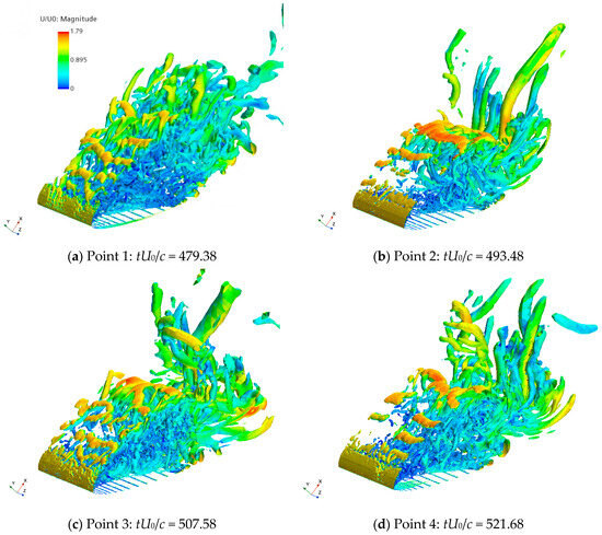
Figure 8.
Instantaneous lambda2 criterion isosurface (λ2 = −4.0 × 10⁵) for NACA0012 sail colored by the relative velocity magnitude at different nondimensional time (points 1–4 correspond to the symbols in Figure 7b, α = 30°, Re = 3.6 × 10⁵).
It can be derived from Figure 8 that the shape of vortices is time-dependent and not uniform in the spanwise direction. The flow structure has strong 3D features, which should not be able to be captured by 2D calculations. For α = 30°, the flow experiences separation upon encountering the leading edge, resulting in the formation of unstable vortices within a triangular region on the lee side of the sail. These vortices originating from the leading edge interact and merge with those emanating from the trailing edge, causing an enlargement in vortex size downstream of the wing sail. As evidenced by Figure 8, the vortices surrounding the wing sail are functions of time. The presence of irregular attached and detached vortices on the sail surface induces erratic fluctuations in the aerodynamic loading experienced by the sail, thereby compromising the stability of the thrust generated.
4.2. Performance of Dynarig Sail and Comparisons with NACA0012
The computed results of CL for α = 15°, 30°, and 45°, and the results of CD for α = 90° of the Dynarig sail are displayed with nondimensional time tU0/c in Figure 9.
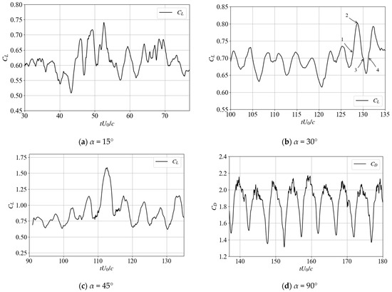
Figure 9.
Nondimensional time history for lift or drag coefficient for different angles of attack (annotations from 1 to 4 in (b) will be used in Figure 10).
Similarly to the NACA0012 sail, the amplitude of wiggles of the force coefficient increases with the rise of attack angle. The changes in the value of CL show in irregular phenomenon with time. However, differently from the NACA0012 sail, the values of CD at α = 90° are close to a state of regular change for the Dynarig sail. This might be caused by differences in sail geometry, which will be further discussed later.
Four instantaneous statuses are illustrated with the lambda2 criterion to demonstrate the vortices of the sail, which are shown in Figure 10. Similarly, this figure is also colored by the relative velocity U/U0.
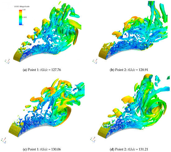
Figure 10.
Instantaneous lambda2 criterion isosurface (λ2 = −2.5 × 10³) for Dynarig sail colored by the relative velocity magnitude at different nondimensional time (points 1–4 correspond to the symbols in Figure 9b, α = 30°, Re = 3.6 × 10⁵).
It can be derived from Figure 10 that the vortex shedding generated by the leading edge exhibits a distinct periodic pattern, developing into a series of intermittent vortices that propagate towards the wake flow. This series of vortices forms one boundary of the trailing vortex region. Furthermore, compared to the NACA0012 sail, the vortices generated by the trailing edge of the Dynarig sail exhibit a more pronounced upward rolling trend. Additionally, due to the relatively larger distance between the leading edge and trailing edge compared to the NACA0012 sail, the influence of the leading-edge vortices on the trailing-edge vortices is diminished. Consequently, the trailing edge of the Dynarig sail can form larger-scale and more complete vortex structures, as illustrated in Figure 10d.
To further analyze the impact of changes in sail geometry on vortices, streamline patterns at mid-slice sections of the NACA0012 and Dynarig are distinctly displayed for α = 15°, 30°, 45°, and 90°, as shown in Figure 11. The streamlines are colored based on the relative velocity (U/U0).
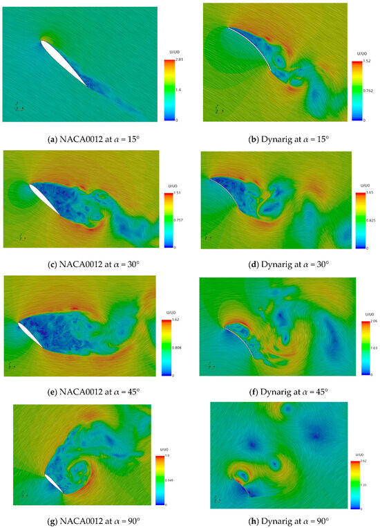
Figure 11.
Streamlines at mid-slice sections for NACA0012 and Dynarig (colored by U/U0).
Based on Figure 11, it can be derived that:
- When α = 15°, the flow is in a transitional state between attached and detached. The separation point for the NACA0012 sail is located towards the rear of the mid-section, whereas the flow close to the leading edge of the Dynarig sail has already fully separated. This suggests that compared to wing sails like the NACA0012, thin-arc sails like the Dynarig are more prone to flow separation as the attack angle increases. Additionally, at this angle of attack, the NACA0012 sail can accelerate the incoming flow up to 2.81-fold, which is more pronounced than the 1.52-fold acceleration caused by the Dynarig sail.
- At α = 30°, the vortex structures of the NACA0012 and Dynarig sails are similar, and their acceleration effects on the flow field are also comparable. This is different from the significant disparity observed at α = 15°, which demonstrates the impact of the sail’s geometric shape on the flow field.
- At α = 45°, the NACA0012 sail generates a more extensive low-speed wake region compared to the Dynarig sail, indicating a state of complete stall. In contrast, the low-speed region in the wake of the Dynarig sail is primarily concentrated near the surface of the sail and in the vicinity of some detached vortices. This phenomenon results in the forces on the Dynarig sail exhibiting more regular variations compared to those on the NACA0012 sail, as reflected in Figure 7c and Figure 9c.
- At α = 90°, where the wind speed is perpendicular to the chord length of the sail, the NACA0012 sail exhibits a large-scale flow-separation region at its trailing end, with no discernible regularity. In contrast, the wake region of the Dynarig sail displays a stronger integrity of vortical structures, as evident from Figure 9d, which also reveals a marked periodicity in the sail’s force fluctuations. This behavior may be attributed to the differences in geometry, specifically the fact that the Dynarig sail possesses a fore–aft symmetric shape, which is geometrically different from the NACA0012 sail.
Nevertheless, the values of CL and CD in Figure 7 and Figure 9 are more likely to change irregularly with time. Limited information can be derived if those results are shown only in the time domain. Therefore, spectrum analysis is conducted to further analyze the composition of the oscillation and the dominant frequency, which are dealt with in the following section.
4.3. Spectrum Analysis for NACA0012 Sail and Dynarig Sail
Oscillations in CL and CD can be seen as superpositions of a certain number of regular signals. In this section, the FFT method is applied to convert the results of CL and CD from the time domain to the frequency domain. Spectrum analysis for the NACA0012 sail and the Dynarig sail at four angles of attack (15°, 30°, 45°, and 90°) are shown in Figure 12 and Figure 13, respectively. “Amplitude” in the figures indicates the absolute value (modulus) of the complex number derived from FFT.
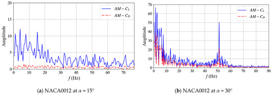
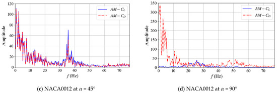
Figure 12.
Spectra for the lift and drag coefficients of the NACA0012 sail at different angles.
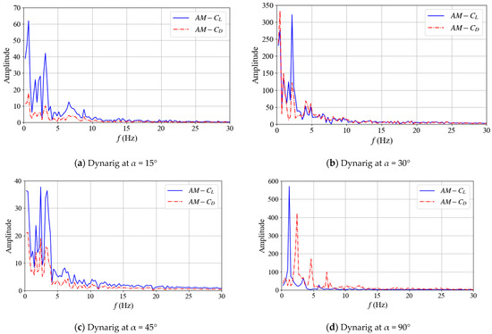
Figure 13.
Spectra for the lift and drag coefficients of the Dynarig sail at different angles.
- For both the NACA0012 and Dynarig, with the increment in attack angle, the amplitudes of CL and CD in the frequency domain also increase. For instance, the maximum amplitude of CL of both NACA0012 and Dynarig sails at α = 90° is about 10 times than that at α = 15°.
- The dominant frequency (with the largest value of amplitude) is located in the range of 0.5–10 Hz, which clearly indicates a low-frequency oscillation.
- For the NACA0012 sail, a second local maximum-frequency region can be found at 30–60 Hz at both α = 30° and α = 45°. This phenomenon is not found for the Dynarig sail, which might be caused by the geometry difference.
- Compared to the NACA0012 sail, the Dynarig sail’s spectrum has significantly fewer local maxima. This implies that the Dynarig sail comprises fewer frequency components when subjected to low-frequency oscillations. Such a distinction can serve as a reference for frequency-based sail selection.
A nondimensional quantity, the Strouhal number (St), is used to illustrate how the dominant frequency changes with angles of attack. St is defined as follows:
where f is the frequency. Based on the FFT analysis, the St in the case of the dominant frequency for each attack angle is shown in Figure 14. Since the dominant frequency for CL and CD is not obvious for α < 15°, values of St are only depicted in the range of 15–90°.
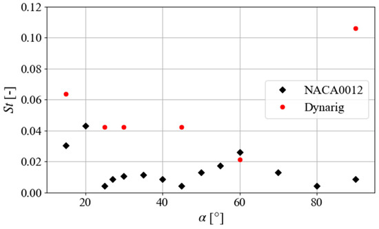
Figure 14.
The Strouhal number in dominant frequency shown against attack angles (Re = 3.6 × 10⁵).
Figure 14 indicates that St values for both types of sails are predominantly below 0.1, signifying a relatively low level, and exhibit a decreasing trend with increasing angles of attack. Except for α = 60°, the dominant frequency corresponding to the St value of the Dynarig sail is higher than that of the NACA0012 sail. At α = 90°, the St of the Dynarig sail is significantly higher than those at other attack angles and is also notably higher than the St of the NACA0012 sail at α = 90°. Based on the frequency distribution in the wake analysis from Figure 11h and Figure 13d, the oscillation frequency components on the Dynarig sail at this state are fewer and concentrated within the range of f < 10 Hz. This may be one of the reasons for a larger St of the Dynarig sail at α = 90°.
It can also be derived based on Figure 14 that the St varies with the attack angle, which means the frequency of the low-frequency oscillations can be controlled by altering the angle of attack. Designers of the unmanned sailboat should keep this information in mind when determining the attack angle in a specific condition.
To evaluate the degree of influence of low-frequency component on the sail force, the percentage of the fluctuation in the total force is computed. Through FFT analysis, the CL and CD corresponding to the dominant frequency can be derived accurately. They are shown as percentages of the time-averaged CL or CD (Figure 15).
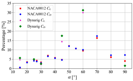
Figure 15.
The magnitude of CL and CD at the dominant frequency shown as the percentage of the averaged CL and CD.
Based on Figure 15, CL and CD in the case of the dominant frequency tend to increase with the attack angle when α ≤ 70°. The latter rises to a maximum of 31.27% of CD at α = 60° for the Dynarig sail and 17.44% of CD at α = 60° for the NACA0012 sail. This means that the amplitude of force fluctuations can deviate 30% and 17% from the time-averaged forces for the Dynarig and NACA0012, respectively, which are too significant to be ignored. Therefore, the effect of these force fluctuations on sail forces should be considered at the primary stage of sail design.
5. Conclusions
In this study, large-eddy simulations are applied at Reynolds number 3.6 × 10⁵ for a 3D NACA0012 sail and compared with the results from a Dynarig sail. The lift and drag coefficients derived from LES computations are presented and discussed for angles of attack in the range of 5° to 90°. Spectrum analysis is applied to find the dominant frequency of the oscillations. Several conclusions can be obtained, as follows.
- For the NACA0012 sail, when α = 15°, the flow is not fully separated. The amplitude of the flow oscillations is suppressed and shows physically stable flow in the wake. With increased attack angle, an increment is also found in the amplitude of the force coefficients, where the oscillating percentage of CL or CD can rise to about 20%, 35%, and 50% for α = 30°, 45° and 90°.
- For the Dynarig sail, the amplitude of wiggles of the force coefficient increases with the rise in attack angle, which is similar to the NACA0012 sail. However, the values of CD at α = 90° are close to a state of regular change for the Dynarig sail.
- For both the NACA0012 and Dynarig, with the increment in attack angle, the amplitude of CL and CD in the frequency domain also increase. Different from the Dynarig sail, a second local maximum-frequency region can be found at 30–60 Hz.
- Compared to the NACA0012 sail, the Dynarig sail’s spectrum has significantly fewer local maxima. Such a distinction can serve as a reference for frequency-based sail selection.
- Strouhal numbers for both sails are predominantly below 0.1, signifying a relatively low level, and exhibit a decreasing trend with increasing angles of attack.
- The amplitude of force fluctuations deviates up to 30% and 17% from the time-averaged forces for Dynarig and NACA0012, respectively, which are too significant to be ignored.
Therefore, the effects of the force fluctuations are significant and should be considered at the primary stage of sail design. In future research, the effects of the sail tip and the deck of the sailboat will be investigated, which are considered to provide a closer approximation of the physical model and give recommendations for unmanned sailboat design and manipulation.
Author Contributions
Conceptualization, Q.Z. and W.C.; methodology, Q.Z.; software, Q.Z.; validation, Q.Z. and J.X.; formal analysis, Q.Z.; investigation, Q.Z.; writing—original draft preparation, Q.Z.; writing—review and editing, W.C.; visualization, J.X. All authors have read and agreed to the published version of the manuscript.
Funding
This research was funded by the Fundamental Research Funds for the Central Universities, grants 40120592 and 3120621209, and Hainan Institute of Wuhan University of Technology, grant 2022KF0022.
Institutional Review Board Statement
Not applicable.
Informed Consent Statement
Not applicable.
Data Availability Statement
Data and models generated or used in this study are available from the corresponding author upon request.
Conflicts of Interest
The authors declare no conflicts of interest.
References
- Meinig, C.; Lawrence-Slavas, N.; Jenkins, R.; Tabisola, H.M. The Use of Saildrones to Examine Spring Conditions in the Bering Sea: Vehicle Specification and Mission Performance. In Proceedings of the OCEANS 2015—MTS/IEEE, Washington, DC, USA, 19–22 October 2015; pp. 1–6. [Google Scholar]
- An, Y.; Yu, J.; Zhang, J. Autonomous Sailboat Design: A Review from the Performance Perspective. Ocean Eng. 2021, 238, 109753. [Google Scholar] [CrossRef]
- Sun, Q.; Qi, W.; Liu, H.; Ji, X.; Qian, H. Toward Long-Term Sailing Robots: State of the Art From Energy Perspectives. Front. Robot. AI 2021, 8, 7253. [Google Scholar] [CrossRef] [PubMed]
- Silva, M.F.; Friebe, A.; Malheiro, B.; Guedes, P.; Ferreira, P.; Waller, M. Rigid Wing Sailboats: A State of the Art Survey. Ocean Eng. 2019, 187, 106150. [Google Scholar] [CrossRef]
- Enqvist, T.; Friebe, A.; Haug, F. Free Rotating Wingsail Arrangement for Åland Sailing Robots. In Robotic Sailing 2016; Springer: Berlin/Heidelberg, Germany, 2017; pp. 3–18. [Google Scholar] [CrossRef]
- Selig, M.S.; Donovan, J.F.; Fraser, D.B. Airfoils at Low Speeds; H.A. Stokely: Virginia Beach, VA, USA, 1989. [Google Scholar]
- Souppez, J.-B.R.G.; Arredondo-Galeana, A.; Viola, I.M. Recent Advances in Numerical and Experimental Downwind Sail Aerodynamics. J. Sail. Technol. 2019, 4, 45–65. [Google Scholar] [CrossRef]
- Almutairi, J.H.; AlQadi, I.M. Large-Eddy Simulation of Natural Low-Frequency Oscillations of Separating-Reattaching Flow near Stall Conditions. AIAA J. 2013, 51, 981–991. [Google Scholar] [CrossRef]
- Eljack, E.M.; Soria, J. Investigation of the Low-Frequency Oscillations in the Flowfield about an Airfoil. AIAA J. 2020, 58, 4271–4286. [Google Scholar] [CrossRef]
- ElJack, E. High-Fidelity Numerical Simulation of the Flow Field around a NACA-0012 Aerofoil from the Laminar Separation Bubble to a Full Stall. Int. J. Comput. Fluid Dyn. 2017, 31, 230–245. [Google Scholar] [CrossRef]
- ElAwad, Y.A.; ElJack, E.M. Numerical Investigation of the Low-Frequency Flow Oscillation over a NACA-0012 Aerofoil at the Inception of Stall. Int. J. Micro Air Veh. 2019, 11, 1756829319833687. [Google Scholar] [CrossRef]
- Arredondo-Galeana, A.; Babinsky, H.; Viola, I.M. Vortex Flow of Downwind Sails. Flow 2023, 3, E8. [Google Scholar] [CrossRef]
- William, Y.E.; Kanagalingam, S.; Mohamed, M.H. Ground Effect Investigation on the Aerodynamic Airfoil Behavior Using Large Eddy Simulation. J. Fluids Eng. 2024, 146, 031205. [Google Scholar] [CrossRef]
- Cravero, C. Aerodynamic Performance Prediction of a Profile in Ground Effect With and Without a Gurney Flap. J. Fluids Eng. 2017, 139, 031105. [Google Scholar] [CrossRef]
- Zhu, H.; Yao, H.-D.; Ringsberg, J.W. Unsteady RANS and IDDES Studies on a Telescopic Crescent-Shaped Wingsail. Ships Offshore Struct. 2024, 19, 134–147. [Google Scholar] [CrossRef]
- Dawi, A.H.; Akkermans, R.A.D. Direct Noise Computation of a Generic Vehicle Model Using a Finite Volume Method. Comput. Fluids 2019, 191, 104243. [Google Scholar] [CrossRef]
- Akkermans, R.A.D.; Ewert, R.; Moghadam, S.M.A.; Dierke, J.; Buchmann, N. Overset DNS with Application to Sound Source Prediction. In Proceedings of the Progress in Hybrid RANS-LES Modelling, College Station, TX, USA, 19–21 March 2015; Girimaji, S., Haase, W., Peng, S.-H., Schwamborn, D., Eds.; Springer International Publishing: Cham, Switzerland, 2015; pp. 59–68. [Google Scholar]
- Zeng, Q.; Cai, W. Simulation and Characterization of Low-Frequency Flow Oscillations Over a Symmetrical Sail at Large Attack Angles for an Unmanned Sailboat. In Proceedings of the ASME 2023 42nd International Conference on Ocean, Offshore and Arctic Engineering, Melbourne, Australia, 11–16 June 2023; American Society of Mechanical Engineers Digital Collection: New York, NY, USA, 2023. [Google Scholar]
- Jabbari, H.; Esmaeili, A.; Rabizadeh, S. Phase Portrait Analysis of Laminar Separation Bubble and Ground Clearance Interaction at Critical (Low) Reynolds Number Flow. Ocean Eng. 2021, 238, 109731. [Google Scholar] [CrossRef]
- Eljack, E.; Soria, J.; Elawad, Y.; Ohtake, T. Simulation and Characterization of the Laminar Separation Bubble over a NACA-0012 Airfoil as a Function of Angle of Attack. Phys. Rev. Fluids 2021, 6, 034701. [Google Scholar] [CrossRef]
- Moise, P.; Zauner, M.; Sandham, N.D. Connecting Transonic Buffet with Incompressible Low-Frequency Oscillations on Aerofoils. J. Fluid Mech. 2024, 981, A23. [Google Scholar] [CrossRef]
- Leonard, A. Energy Cascade in Large-Eddy Simulations of Turbulent Fluid Flows. In Advances in Geophysics; Frenkiel, F.N., Munn, R.E., Eds.; Turbulent Diffusion in Environmental Pollution; Elsevier: Amsterdam, The Netherlands, 1975; Volume 18, pp. 237–248. [Google Scholar]
- Abbott, I.H.; von Doenhoff, A.E. Theory of Wing Sections: Including a Summary of Airfoil Data; Courier Corporation: North Chelmsford, MA, USA, 2012; ISBN 978-0-486-13499-4. [Google Scholar]
- Zeng, Q.; Hekkenberg, R.; Thill, C.; Hopman, H. Scale Effects on the Wave-Making Resistance of Ships Sailing in Shallow Water. Ocean Eng. 2020, 212, 107654. [Google Scholar] [CrossRef]
- Eça, L.; Hoekstra, M. A Procedure for the Estimation of the Numerical Uncertainty of CFD Calculations Based on Grid Refinement Studies. J. Comput. Phys. 2014, 262, 104–130. [Google Scholar] [CrossRef]
- Zeng, Q.; Zhang, X.; Cai, W.; Zhou, Y. Wake Distortion Analysis of a Dynarig and Its Application in a Sail Array Design. Ocean Eng. 2023, 278, 114341. [Google Scholar] [CrossRef]
- Sheldahl, R.E.; Klimas, P.C. Aerodynamic Characteristics of Seven Symmetrical Airfoil Sections through 180-Degree Angle of Attack for Use in Aerodynamic Analysis of Vertical Axis Wind Turbines; Sandia National Labs.: Albuquerque, NM, USA, 1981. [Google Scholar]
Disclaimer/Publisher’s Note: The statements, opinions and data contained in all publications are solely those of the individual author(s) and contributor(s) and not of MDPI and/or the editor(s). MDPI and/or the editor(s) disclaim responsibility for any injury to people or property resulting from any ideas, methods, instructions or products referred to in the content. |
© 2024 by the authors. Licensee MDPI, Basel, Switzerland. This article is an open access article distributed under the terms and conditions of the Creative Commons Attribution (CC BY) license (https://creativecommons.org/licenses/by/4.0/).