Article

Robust Fixed-Time Fault-Tolerant Control for USV with Prescribed Tracking Performance

Navigation College, Jimei University, Xiamen 361021, China
*
Author to whom correspondence should be addressed.
J. Mar. Sci. Eng. 2024, 12(5), 799; https://doi.org/10.3390/jmse12050799
Submission received: 20 March 2024 / Revised: 28 April 2024 / Accepted: 6 May 2024 / Published: 10 May 2024

Abstract

:
The unmanned surface vessel (USV) is an emerging marine tool with its advantages of automation and intelligence in recent years; the good trajectory tracking performance is an important capability. This paper proposes a novel prescribed performance fixed-time fault-tolerant control scheme for an USV with model parameter uncertainties, unknown external disturbances, and actuator faults, based on an improved fixed-time disturbances observer. Firstly, the proposed observer can not only accurately and quickly estimate and compensate the lumped nonlinearity, including actuator faults, but also reduce the chattering phenomenon by introducing the hyperbolic tangent function. Then, under the framework of prescribed performance control, a prescribed performance fault-tolerant controller is designed based on a nonsingular fixed-time sliding mode surface, which guarantees the transient and steady-state performance of an USV under actuator faults and meets the prescribed tracking performance requirements. In addition, it is proved that the closed-loop control system has fixed-time stability according to Lyapunov’s theory. Finally, upon conducting numerical simulations and comparing the proposed control scheme with the SMC and the finite-time NFTSMC scheme, it is evident that the absolute error tracking performance index of the proposed control scheme is significantly lower, thus indicating its superior accuracy.

1. Introduction

In recent years, the unmanned surface vessel (USV) has been extensively utilized in ocean sampling, ocean mapping, and maritime rescue owing to its compact size, exceptional maneuverability, and effective concealment [1]. A requirement of the USV in performing the above tasks is to be able to arrive and remain precisely on the desired trajectory within the specified time. However, there are significant challenges in achieving precise trajectory tracking for the USV. Firstly, the dynamics of the USV exhibit highly nonlinear behavior. Secondly, the exact model of the USV system is unknown, and working conditions are often harshly affected by sea winds, waves, and currents [2]. Accurate trajectory tracking is crucial for the safe and efficient autonomous operation of the USV in different scenarios and thus has important research value and practical significance.
At present, the trajectory tracking control methods of the USV mainly include the following: PID control [3], backstepping control [4,5], fuzzy control [6], adaptive control [7,8], and sliding mode control (SMC) [9,10,11]. In particular, SMC has been proven to be highly robust to uncertainties and disturbances in nonlinear systems, and it is widely used in ship trajectory tracking control. For example, by introducing a disturbance observer to estimate the disturbance and compensate it in the control law and combining it with SMC, the trajectory tracking of the USV was implemented in [12]. Similarly, Piao et al. [13] proposed an adaptive backstepping SMC strategy that used the adaptive law to estimate the bounds of the external unknown disturbance. But the upper bound of the disturbance is known and constant. Furthermore, Chen et al. [14] designed an adaptive sliding mode controller by combining radial basis function neural networks (RBFNNs), which were used to approximate and compensate modeling uncertainties, and a disturbance observer to estimate and compensate external disturbances. However, these SMC methods all choose a linear sliding surface, which can only guarantee that the tracking error converges to zero asymptotically, and the convergence rate can be adjusted by adjusting the sliding mode surface parameters, while the system tracking error cannot converge to zero in finite time regardless.
In order to speed up the error convergence, finite-time control methods [15,16,17] have been widely used in the field of USV motion control. Also of relevance, Xu et al. [18] proposed a nonsingular fast terminal SMC scheme based on a finite-time extended state observer (ESO). In [19], the universal approximation property of RBFNNs was used to estimate the uncertainty of the system, and event-triggered control (ETC) and finite-time control were combined to solve the problem of system uncertainty and asymmetric input saturation. Then, Rodriguez et al. [20] designed a finite-time control strategy by combining adaptive boundary estimation and the integral SMC method. Furthermore, Huang et al. [21] used RBFNNs to approximate the uncertain system dynamics and used the minimum learning parameter (MLP) algorithm to reduce the computational complexity. At the same time, by introducing a finite-time SMC algorithm, the finite-time formation control of the USV was realized. Notably, it should be pointed out that the tracking error convergence time in the above control method depends on the control parameters and the initial state of the system, which indicates that when the control parameters are unchanged and the initial error of the system tends to infinity, the error convergence time will also increase unbounded. In order to make the upper bound on the convergence time of the system independent of the initial state, the fixed-time control was first proposed by the researcher Polyakov in [22]. Inspired by this, Yao et al. [23] proposed a fixed-time terminal SMC scheme, and the trajectory tracking error of USV can converge in a fixed time, but this fixed-time terminal sliding mode surface will produce singularity. In view of this, a nonsingular fixed-time terminal SMC strategy was proposed in [24]. Additionally, Chen et al. [25] proposed a nonsingular fixed-time fractional order sliding mode controller and introduced RBFNNs to estimate external disturbances. However, when using neural networks to approximate unknown external disturbances, it is a difficult problem to select the weighting matrix and the number of hidden layer nodes.
In practical engineering applications, it is necessary to consider actuator faults in order to ensure the performance and reliability of USV tracking control. Actuator fault is known as one of the most typical cases of input constraints, which may degrade the control performance, especially for USV motion control systems that require high safety. Therefore, fault-tolerant control (FTC) techniques must be considered. In [26], actuator faults of the USV are addressed by auxiliary systems integrated with adaptive techniques. In addition, Zhang et al. [27] transformed the dynamic model with actuator faults and uncertainties into a nominal model with equivalent disturbances and tracked by a robust compensator. In [28], a fault efficiency estimator is constructed based on a fuzzy-aided nonlinear observer.
The above studies have achieved certain results in improving the steady-state accuracy of USV trajectory tracking, but less consideration has been given to the transient performance and output constraints of trajectory tracking errors, especially for the transient performance (such as overshoot) of trajectory tracking under actuator faults. Heshmati-Alamdari et al. [29] proposed a prescribed performance control (PPC) strategy to achieve trajectory tracking under prescribed transient and steady-state responses without considering the model’s uncertainties and external disturbances.
In summary, in order to highlight the difference between this paper and existing related studies, Table 1 indicates that the controller considers multiple factors. Note that if the controller satisfies the factor in Table 1, it is marked by ✓, otherwise, by ⨯.
In this work, an improved fixed-time disturbances observer-based prescribed performance fixed-time fault-tolerant control (IFxDO-PPFxFC) scheme is proposed to solve the problem that the tracking control results of the USV are susceptible to the initial states of the system, unknown external disturbances, model parameter uncertainties, and actuator faults. Then, the main contributions of this paper are as follows:
(1)
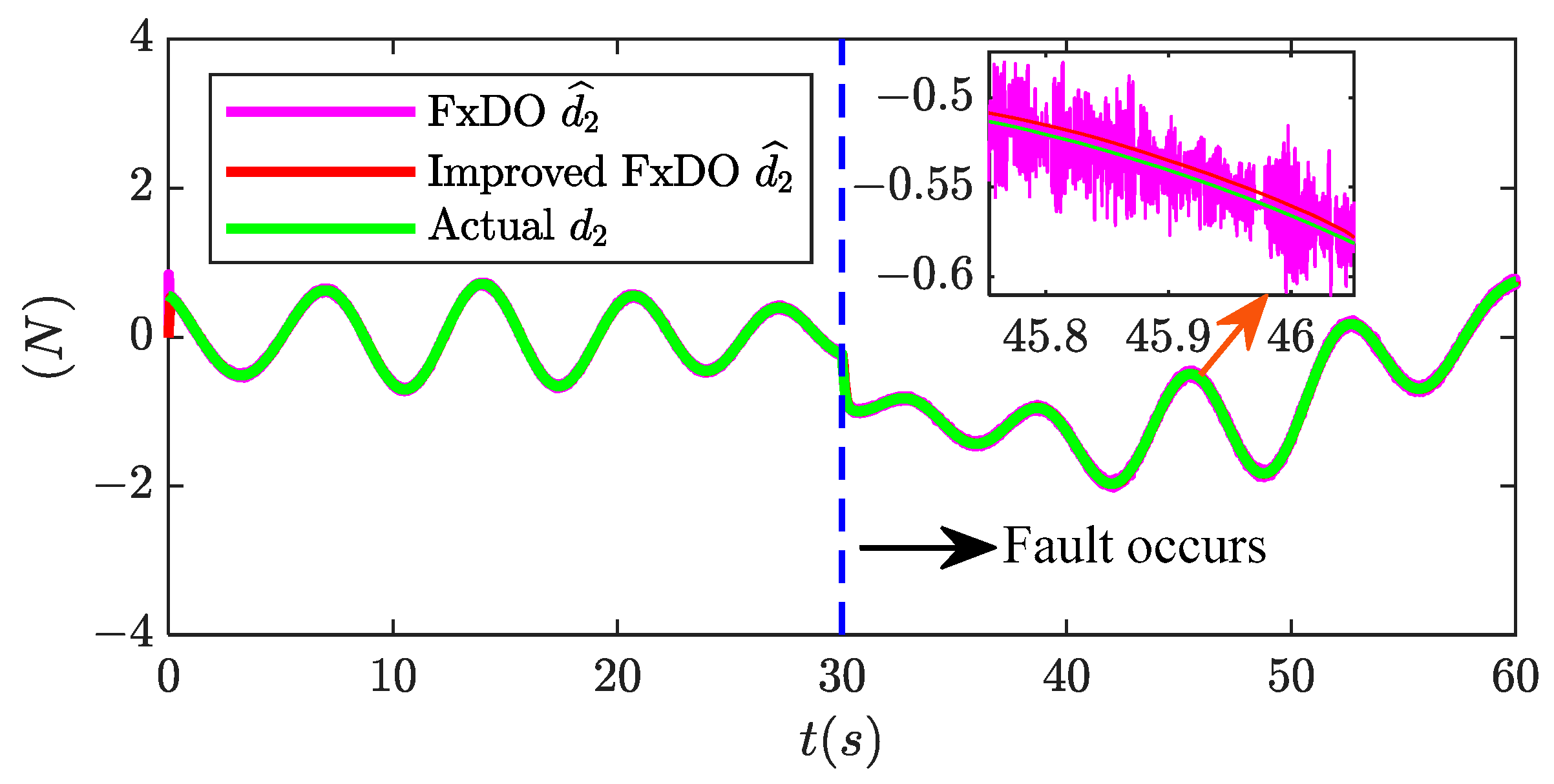
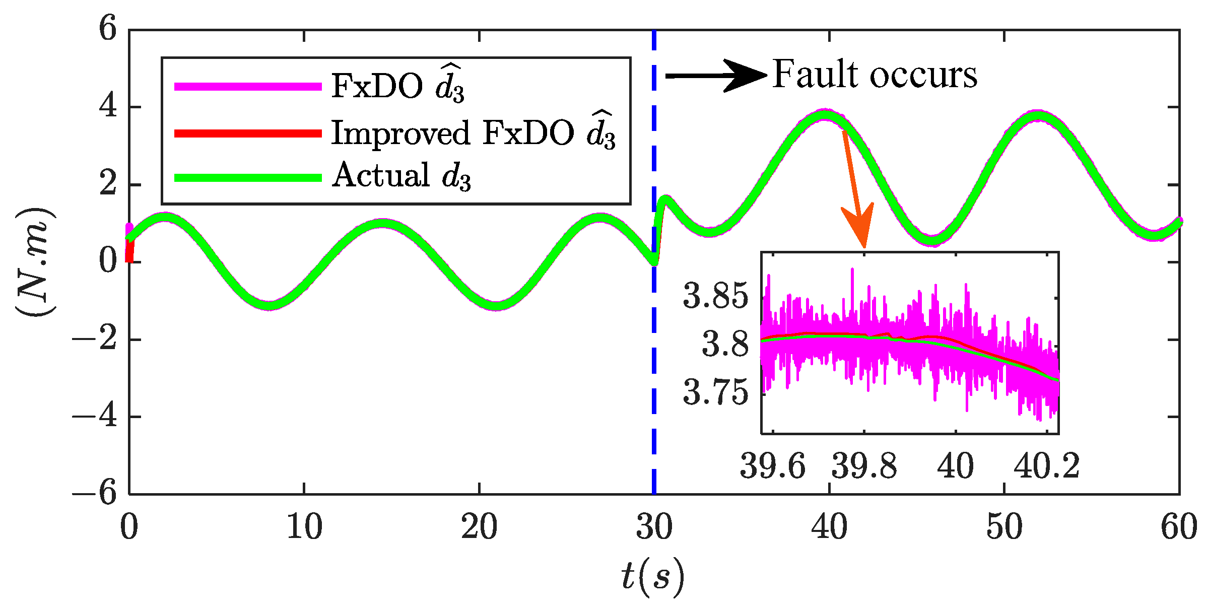
An improved fixed-time disturbances observer is proposed. The proposed technique is significant in that it not only provides faster convergence but also effectively reduces the chattering phenomenon by introducing the hyperbolic tangent function. In addition, the bound of the convergence time value can be predicted in advance.
(2)
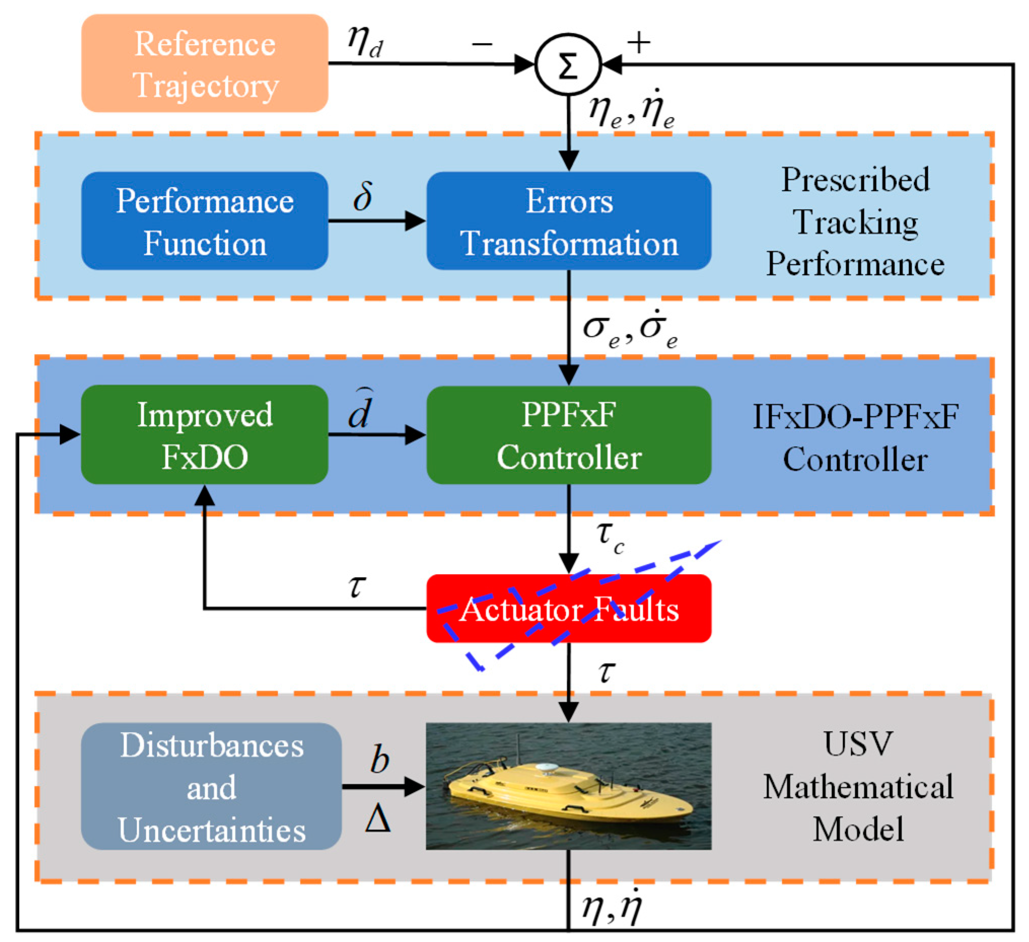
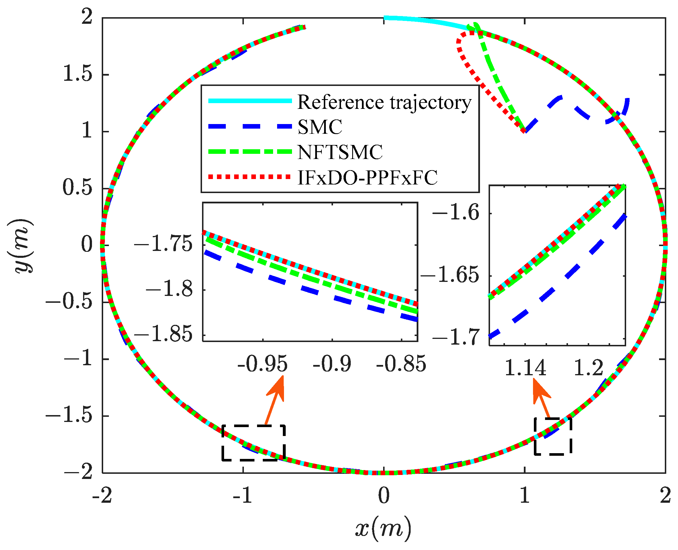
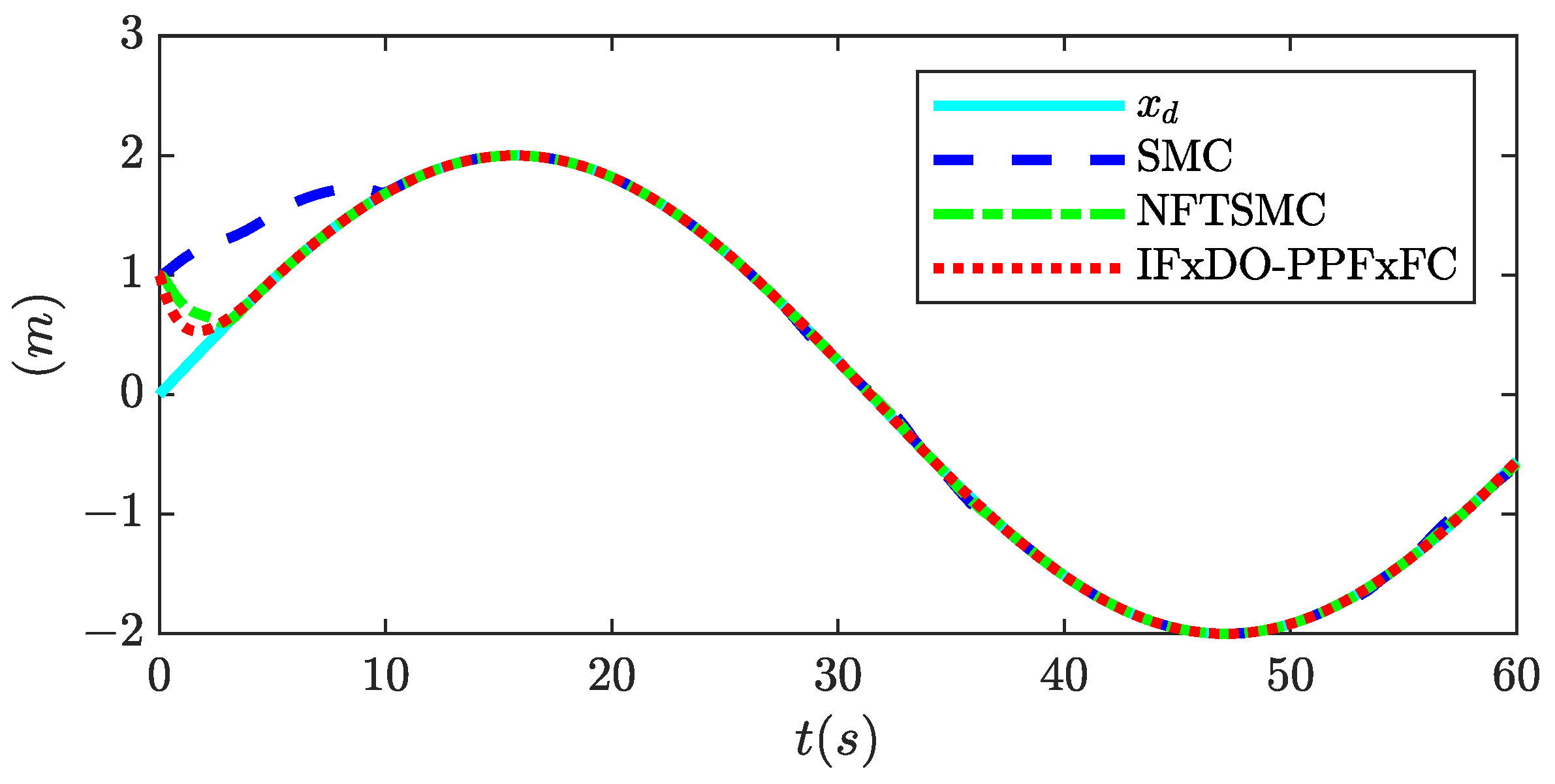
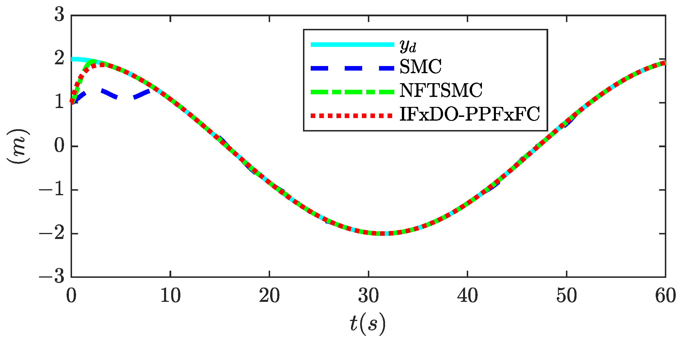
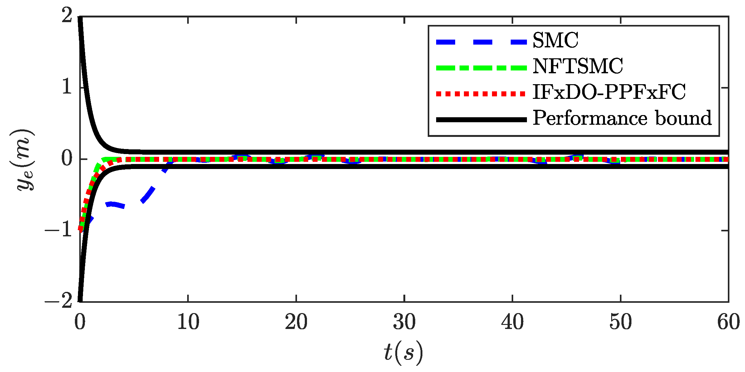
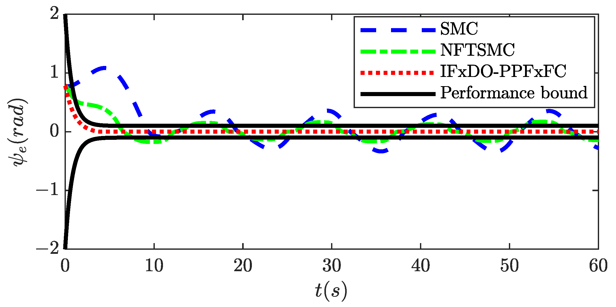
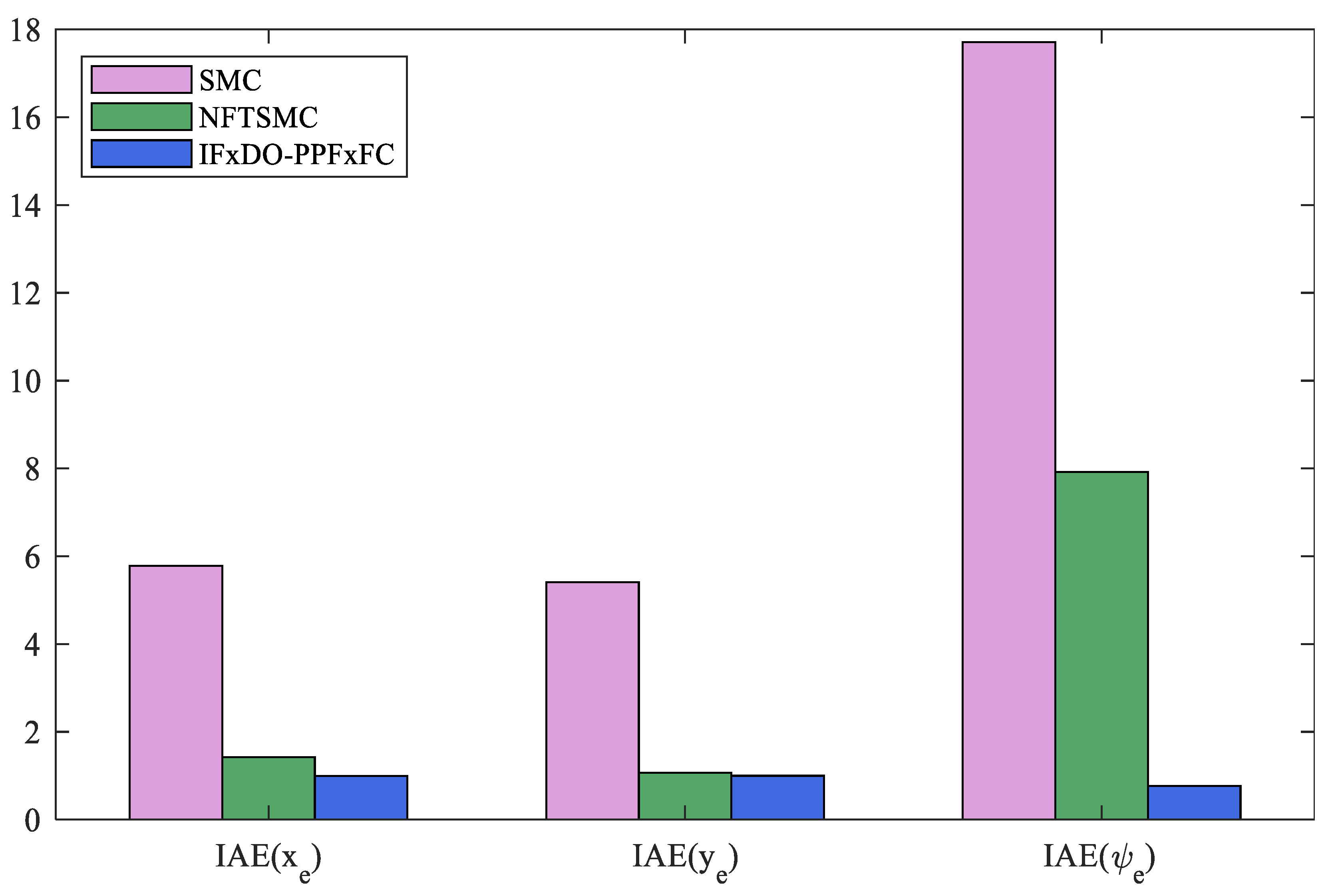
Combining fixed-time SMC, FTC, and PPC theories, a novel IFxDO-PPFxFC scheme is proposed in this paper. Unlike the finite-time stable control scheme [18,19,20], The proposed control scheme enables the USV to accurately track the desired trajectory in a fixed time, and the convergence time is independent of initial states. Meanwhile, the advantage of this control scheme is its singularity-free. Furthermore, it can guarantee the transient and steady-state performance of output errors of trajectory tracking controller even in the presence of actuator faults; this is of great significance for the safe navigation of USV.
This paper is organized as follows. Section 2 gives the preliminaries and problem formulation. Section 3 presents the controller design and stability analysis. Section 4 verifies it through simulation experiments. Finally, Section 5 gives the conclusions.

2. Preliminaries and Problem Formulation

In this section, in order to facilitate the subsequent controller design and stability proofs, we present the needed notations, definitions, and lemmas for the controller design, introducing the detailed mathematical model of the USV.

2.1. Preliminaries

Notations: 
n  denotes an  n × 1  column vector,  n × m  denotes an  n × m  dimensional matrix,  λ max ( · )  and  λ min ( · )  denote the minimum and maximum eigenvalue of a matrix,  d i a g ·  denotes the diagonal matrix,  ·  denotes the modulus of a vector, and  ·  denotes the 2-norm of a vector or the induced norm of a matrix, respectively. For a vector  x = x 1 , x 2 , x n T n  and a positive scalar  a , s i g n ( x ) = s i g n ( x 1 ) , s i g n ( x 2 ) s i g n ( x n ) T x a = x 1 a   s i g n ( x 1 ) , x 2 a   s i g n ( x 2 ) x n a   s i g n ( x n ) T  and  x a = x 1   a , x 2   a x n   a ) T , where  s i g n ( x )  denotes the signum function.
Definition 1.
Consider the following system:
y ˙ = f ( y ) , y ( 0 ) = y 0 , y n
The origin of the system (1) is said to be fixed-time stable if there exists a bounded constant T which is independent of the initial value such that
lim t T y = 0 , y = 0   f o r   t > T
Lemma 1
([30]). For the system (1), assume that there exists a positive definite continuous Lyapunov function that satisfies
V ˙ ( y ) λ 1 V α ( y ) λ 2 V β ( y )
where  λ 1 > 0 , λ 2 > 0 , 0 < α < 1 , and β > 1 . The system (1) is globally fixed-time stable, ensuring that the convergence time  T  satisfies
T T ( α , β , λ 1 , λ 2 ) = 1 λ 1 ( 1 α ) + 1 λ 2 ( β 1 )
Lemma 2
([31]). For the system (1), assume that there exists a positive definite continuous Lyapunov function that satisfies
V ˙ ( y ) a V p ( y ) b V q ( y ) + ε
where  a  and  b  are positive constants,  0 < p < 1 ,  q > 1 , and  0 < ε < . Then, the system (1) is practically fixed-time stable, and the system state can converge to the residual set at fixed time
lim y T y V ( y ) min a 1 p ε 1 θ 1 p , b 1 p ε 1 θ 1 q
where  θ  is a positive constant and satisfies  0 < θ < 1 . The system convergence time  T  satisfies
T T ( a , b , p , q ) = 1 a ( 1 p ) + 1 b ( q 1 )
Lemma 3
([32]). If  ε 1 , ε 2 , , ε n 0 , there exists
i = 1 n ε i   p i = 1 n ε i κ , 0 < κ < 1
i = 1 n ε i   p n 1 p i = 1 n ε i κ , κ > 1 .

2.2. USV Mathematical Model

In general, the motion of the USV in the horizontal plane is regarded as the 3-DOF motion, namely surge, sway, and yaw. As shown in Figure 1, the kinematic model parameters of the USV are established based on the earth-fixed O X Y and the body-fixed O E X E Y E coordinate frames.
The kinematic and dynamic models of the USV are defined as follows [33]:
η ˙ = R ( ψ ) v M v ˙ = C ( v ) v D ( v ) v + τ + b
where η = x y ψ T 3 is the position and heading of the USV in the earth-fixed frame. v = u v r T 3 is the surge, sway, and yaw velocities of the USV in the body-fixed frame. τ = τ 1 τ 2 τ 3 T 3 is the control input. b = b u b v b r T 3 is the external environmental unknown time-varying disturbance. The rotation matrix R ( ψ ) 3 × 3 is given as follows:
R ( ψ ) = cos ψ sin ψ 0 sin ψ cos ψ 0 0 0 1
The matrix R ( ψ ) has the following properties: R ˙ ( ψ ) = R ( ψ ) S ( r ) , R T ( ψ ) S ( r ) R ( ψ ) = R ( ψ ) S ( r ) R ( ψ ) T = S ( r ) , R ( ψ ) = 1 . The matrix S ( r ) is given as follows:
S ( r ) = 0 r 0 r 0 0 0 0 0
M 3 × 3 is the positive definite matrix, and it satisfies M = M T > 0 . Its expression is
M = m 11 0 0 0 m 22 m 23 0 m 32 m 33
where m 11 = m X u ˙ , m 22 = m Y v ˙ , m 23 = m x g Y r ˙ , m 32 = m x g N v ˙ , and m 33 = I z N r ˙ .
C ( v ) 3 × 3 is the Coriolis and centripetal matrix, and it satisfies C ( v ) = C ( v ) T > 0 .   D ( v ) 3 × 3 is the damping matrix. They are expressed as follows:
C ( v ) = 0 0 c 13 ( v ) 0 0 c 23 ( v ) c 13 ( v ) c 23 ( v ) m 33 , D ( v ) = d 11 ( v ) 0 0 0 d 22 ( v ) d 23 ( v ) 0 d 32 ( v ) d 33 ( v )
where c 13 ( v ) = m 11 v m 23 r , c 23 ( v ) = m 11 u , d 11 ( v ) = X u X   u u u X u u u u 2 , d 22 ( v ) = Y v Y v v v Y r v r , d 23 ( v ) = Y r Y v r v Y r r r , d 32 ( v ) = N v N v v v N r v r , and d 33 ( v ) =   N r N v r v N r r r , where m is the mass of the USV, I z is the moment of inertia, and x g is the distance from the center of gravity to the origin on the Y . X , Y , and N are the hydrodynamic parameters acting on the USV.
According to the research of Zhang et al. [27], the control input of the USV with actuator faults can be expressed by the following mathematical method:
τ i = τ c i + f ( t T 0 i ) e i 1 τ c i + τ ¯ i
where τ i ( i = u , v , r ) represents the actual control input acting on the USV, τ c i is the desired control forces and moments, τ ¯ i is the additive uncertain fault input, e i is the thruster efficiency factor with 0 e i 1 , and f ( t T 0 i ) represents the time-varying fault. Its expression is
f ( t T 0 i ) = 0 , t < T 0 i 1 e a i ( t T 0 i ) , t T 0 i
where a i is the unknown fault change rate, and T 0 i is the fault occurrence time of each degree of freedom.
In summary, the equivalent control forces and moments of the USV propulsion system considering the thruster fault constraint is expressed as follows:
τ = τ c + F ( t T 0 ) E I 3 τ c + τ ¯
where F ( t T 0 ) = d i a g f ( t T 0 u ) , f ( t T 0 u ) , f ( t T 0 r ) 3 × 3 is the time-varying fault matrix of the propulsion system. E = d i a g e u , e v , e r 3 × 3 is the efficiency matrix of the propulsion system, τ c = τ c u τ c v τ c r T 3 is the desired control forces and moments vector, and τ ¯ = τ ¯ u τ ¯ v τ ¯ r T 3 is the additive fault vector.
In addition, consider the model parameter uncertainties:
C ( v ) = C 0 ( v ) + Δ C ( v ) D ( v ) = D 0 ( v ) + Δ D ( v )
where C 0 ( v ) and D 0 ( v ) denote the nominal values of the Coriolis and centripetal matrix and the damping matrix, respectively. Δ C ( v ) and Δ D ( v ) denote the uncertainty values of the Coriolis and centripetal matrix and the damping matrix, respectively.
Define an auxiliary velocity vector and let
ω = R ( ψ ) v
where ω = ω 1 ω 2 ω 3 T 3 .
Combining Equations (17) and (18), the mathematical model of the USV can be redefined as follows:
η ˙ = ω ω ˙ = H η , v + R M 1 τ c + d
where H η , v 3 is the total nominal component, d = d 1 d 2 d 3 T 3 is the unknown lumped nonlinearity (model parameter uncertainties, unknown external disturbances, and actuator faults) of the system. They are given as follows:
H η , v = R M 1 M S v C 0 ( v ) v D 0 ( v ) v
d = R M 1 F ( t T 0 ) E I 3 τ c + τ ¯ + b Δ C ( v ) v Δ D ( v ) v
Assumption 1.
The unknown lumped nonlinearity  d  (22) is limited by  d < a , where  a  is an unknown constant. The first-order derivative of  d  is bounded by  d ˙ < b , where  b is a known positive constant.

3. Controller Design and Stability Analysis

In this section, Figure 2 presents the trajectory tracking controller framework diagram for the USV. It is mainly made up of the performance function, an improved FxDO, and a PPFxF controller. The performance function provides the tracking error transformation. The improved FxDO can accurately estimate lumped disturbances and faults in a fixed time. The PPFxF controller makes trajectory tracking errors reach zero at a fixed time and ensures that the transient performance and steady-state performance meet the specified requirements.

3.1. Improved Fixed-Time Disturbances Observer

Notably, when the USV performs its mission in the actual ocean environment, its stability can be seriously affected by unknown disturbances such as wind, waves, and currents. At the same time, the faults of the actuator cannot be ignored. In view of this, by combining the mathematical model of the USV, a fixed-time disturbances observer (FxDO) is applied to estimate and compensate the lumped nonlinearity, including actuator faults, and the observer is designed accordingly as follows:
ω ˜ = ω ω , d ˜ = d d ω ˙ = H η , v + R M 1 τ c + d + ς 1 ω ˜ α 1 s i g n ω ˜ + σ 1 ω ˜ β 1 s i g n ω ˜ d ˙ = ς 2 ω ˜ α 2 s i g n ω ˜ + σ 2 ω ˜ β 2 s i g n ω ˜ + γ s i g n ω ˜
Remark 1.
In Equation (23),  ς 1 ω ˜ α 1 s i g n ω ˜ , σ 1 ω ˜ β 1 s i g n ω ˜ , ς 2 ω ˜ α 2 s i g n ω ˜ , and  σ 2 ω ˜ β 2 s i g n ω ˜  are continuous regardless of the sign function; however,  γ s i g n ω ˜  is discontinuous, leading to a chattering phenomenon. The fixed-time observer’s estimate of the centralized uncertainty will be compensated for in the control input, so the discontinuity term in Equation (23) will cause discontinuities in the control input, which will lead to the chattering phenomenon.
To avoid the problem of the chattering phenomenon, the signum function is approximated in this paper by the hyperbolic tangent function. An improved FxDO can be expressed as follows:
ω ˜ = ω ω , d ˜ = d d ω ˙ = H η , v + R M 1 τ c + d + ς 1 ω ˜ α 1 s i g n ω ˜ + σ 1 ω ˜ β 1 s i g n ω ˜ d ˙ = ς 2 ω ˜ α 2 s i g n ω ˜ + σ 2 ω ˜ β 2 s i g n ω ˜ + γ tanh ω ˜
Theorem 1.
If Assumption 1 is satisfied, the improved FxDO (24) is designed to achieve an accurate estimation of unknown lumped nonlinearity within a fixed time  T d .
The estimated errors are given as follows:
ω ˜ ˙ = ς 1 ω ˜ α 1 s i g n ω ˜ σ 1 ω ˜ β 1 s i g n ω ˜ + d ˜ d ˜ ˙ = ς 2 ω ˜ α 2 s i g n ω ˜ σ 2 ω ˜ β 2 s i g n ω ˜ γ tanh ω ˜ + d ˙
where 0 < α 1 < 1 , 0 < α 2 < 1 , β 1 > 1 , β 2 > 1 , and γ > b . The options for ς 1 , ς 2 , σ 1 , and σ 2 are as follows:
A = ς 1 1 ς 2 0 , B = σ 1 1 σ 2 0
Matrices A and B satisfy the Hurwitz matrix, and it has been proved in [34] that the estimation error of the system converges to zero at fixed time T d , and it is given as follows:
T d λ max 1 a 1 ( P 1 ) λ max ( P 1 ) ( 1 a 1 ) λ min ( Q 1 ) + λ max ( P 2 ) ( b 1 1 ) λ min b 1 1 ( P 1 ) λ min ( Q 2 )
where 1 c 1 < a 1 < 1 , 1 < b 1 < 1 + c 2 , 0 < c 1 < 1 , and c 2 > 0 . P 1 , P 2 , Q 1 , and Q 2 are symmetric positive definite matrixes and satisfy A 1 T P 1 + P 1 A 1 = Q 1 , A 2 T P 2 + P 2 A 2 = Q 2 .

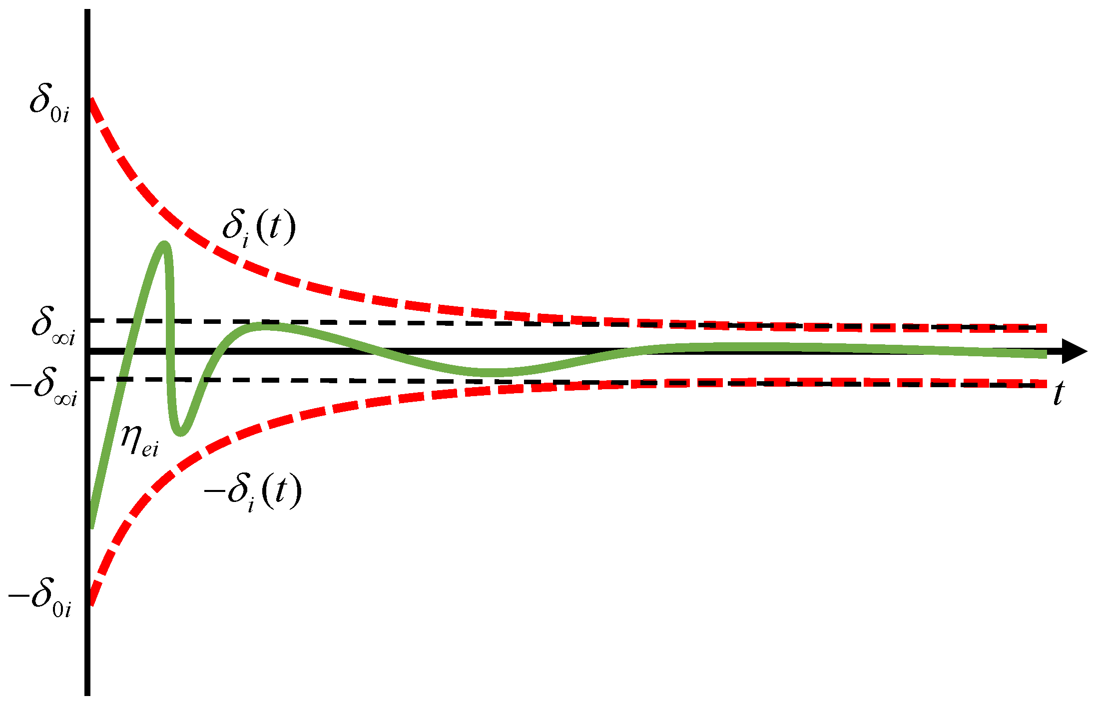
3.2. Errors Transformation via Performance Function

The trajectory tracking errors of the USV are defined as follows:
η e = η η d ω e = η ˙ η ˙ d
where η e = η e u η e v η e r T 3 , ω e = ω e u ω e v ω e r T 3 .
Taking the derivative of Equation (28), the mathematical equation of the tracking errors of the USV can be written as follows:
η ˙ e = ω e ω ˙ e = H η , v + R M 1 τ c + d η ¨ d
where η d = x d y d ψ d T 3 . η d is the desired trajectory, η ˙ d and η ¨ d are the first-order and second-order derivatives of the desired trajectory.
Assumption 2.
The desired trajectory of the USV  η d  is bounded and derivable, and its derivatives  η ˙ d  and  η ¨ d  are smooth and bounded.
In order to ensure that the transient and steady-state performance of the trajectory error η e i is as shown in Figure 3, a prescribed performance function is introduced to constrain the tracking error. Select the following performance function
δ i ( t ) = ( δ 0 i δ i ) exp ( ξ t ) + δ i , ( i = u , v , r )
where ξ is the index of the rate of convergence; researchers can change this index to obtain the prescribed transient and steady-state performance according to the specific needs of the task. δ 0 i denotes the initial value of the prescribed performance function δ i ( t ) , and δ i is the stabilized value after the convergence of the prescribed performance function δ i ( t ) .
Then, a boundary function is constructed from the performance function to limit the tracking error of the system as follows:
f 1 δ i ( t ) < η e i < δ i ( t ) , η e i ( 0 ) 0 δ i ( t ) < η e i < f 2 δ i ( t ) , η e i ( 0 ) 0 , ( i = u , v , r )
From Equation (31), one has
f 1 < η e i δ i ( t ) < 1 , η e i ( 0 ) 0 1 < η e i δ i ( t ) < f 2 , η e i ( 0 ) 0
Assumption 3.
([35]). The initial states of the USV satisfy  δ i ( 0 ) < η e i ( 0 ) < δ i ( 0 ) .
The transformation is achieved by rewriting the tracking error to the following equivalent form
η e i = δ i ( t ) Γ ( σ e i )
where Γ ( σ e i ) is the unconstrained transformation function, σ e i is the transformed error, and δ i ( t ) , Γ ( σ e i ) need to satisfy the following requirements:
  • δ i ( t )  is a monotonically decreasing function;
  • Γ ( σ e i ) ( 1 , 1 ) , Γ ( σ e i ) is a strictly increasing function;
  • δ i ( t ) > 0 , t 0 ;
  • lim σ e i Γ ( σ e i ) = 1 , lim σ e i Γ ( σ e i ) = 1 .
The transformation function in the form of a hyperbolic tangent is defined as follows:
Γ ( σ e i ) = e σ e i f 1 e σ e i e σ e i + e σ e i , σ e i 0 f 2 e σ e i e σ e i e σ e i + e σ e i , σ e i 0
According to the properties of the hyperbolic tangent function, the transformed error can be expressed as
σ e i = Γ 1 η e i δ i ( t ) = 1 2 ln 1 + η e i δ i 1 η e i δ i
The first-order derivative and the second-order derivative of σ e i are calculated as
σ ˙ e i = 1 2 δ ˙ i + η ˙ e i δ i + η e i + δ ˙ i η ˙ e i δ i η e i σ ¨ e i = 1 2 δ ¨ i δ i + η e i δ i + η e i 2 δ i + η e i 2 δ ¨ i δ i η e i δ i η e i 2 δ i η e   i 2 + 1 2 δ i + η e i δ i + η e i 2 δ i η e i δ i η e i 2 ω ˙ e i
For the convenience of the subsequent control design, let
σ ¨ e i = i + ƛ i ω ˙ e i
where
i = δ ¨ i δ i + η e i δ i + η e i 2 / 2 δ i + η e i 2 δ ¨ i δ i η e i δ η e i 2 / 2 δ i η e i 2 ƛ i = δ i + η e i / 2 δ i + η e i 2 δ i η e i / 2 δ i η e i 2 .
Remark 2.
The error transformation by means of a prescribed performance function and the error  η e i  also converges if the error  σ e i  converges. Meanwhile,  δ i ( t )  and  δ i ( t )  limit the maximum overshooting of  η e i  , and the decreasing speed of  δ i ( t )  affects the convergence speed of  η e i . δ i  and  δ i  limit the steady state error of  η e i , so that the prescribed performance control ensures the transient and steady state performance of the error  η e i  at the same time.

3.3. Fixed-Time Fault-Tolerant Controller Design

In order to realize the accurate tracking of the desired trajectory in a fixed time, the sliding surface is constructed according to the errors after the transformation of the prescribed performance function. A nonsingular fixed-time sliding surface s is designed as follows [36]:
s = σ e + 1 λ 1   α σ ˙ e + λ 2 σ e β 1 α
where s = s 1 s 2 s 3 T 3 , σ e = σ e u σ e v σ e r T 3 , 1 / 2 < α < 1 , β > 1 , λ 1 > 0 , and λ 2 > 0 .
Theorem 2.
For the nonlinear USV dynamics system (20), in the presence of actuator faults and model parameter uncertainties given by Equations (17) and (18), if the sliding mode surface is designed as (39), then the closed-loop system is stable, and the errors  σ e  and  σ ˙ e can converge to zero at a fixed time  T s .
Proof. 
When the sliding mold surface s = 0 is reached, which yields
σ ˙ e = λ 1 σ e α λ 2 σ e β
Select the Lyapunov function as follows:
V 1 = 1 2 σ e   T σ e
The derivative of Equation (41) is taken as follows:
V ˙ 1 = 1 2 σ e   T σ ˙ e = σ e   T λ 1 σ e α λ 2 σ e β = λ 1 σ e α + 1 λ 2 σ e β + 1 = λ 1 2 α + 1 / 2 V 1   α + 1 / 2 λ 2 2 β + 1 / 2 V 1   β + 1 / 2 λ 1 2 α / 2 V 1   α + 1 / 2 λ 2 2 β / 2 V 1   β + 1 / 2
Due to 1 / 2 < α < 1 , β > 1 , according to Lemma 1, σ e , σ ˙ e will converge to zero at a fixed time T s , as shown in the following:
T s 2 1 α / 2 λ 1 ( 1 α ) + 2 1 β / 2 λ 2 ( β 1 )
Then, taking the derivative of Equation (39), the following can be obtained:
s ˙ = σ ˙ e + 1 α λ 1   α d i a g σ ˙ e + λ 2 σ e β 1 α 1 σ ¨ e + λ 2 β d i a g σ e β 1 σ ˙ e
Let F ( σ e , σ ˙ e ) = d i a g σ ˙ e + λ 2 σ e β , substituting Equation (37) into Equation (44), the following can be obtained:
s ˙ = σ ˙ e + 1 α λ 1   α F ( σ e , σ ˙ e ) 1 α 1 h + d i a g ƛ i ω ˙ e + λ 2 β d i a g σ e β 1 σ ˙ e
where  h = u v r T 3 , d i a g σ e β 1 = d i a g σ e u β 1 , σ e v β 1 , σ e r β 1 , and d i a g ƛ i = d i a g ƛ u ƛ v r . □
According to Equation (29), Equation (45) can be transformed into
s ˙ = σ ˙ e + 1 α λ 1   α F ( σ e , σ ˙ e ) 1 α 1 h + d i a g ƛ i H η , v + R M 1 τ c + d η ¨ d + λ 2 β d i a g σ e β 1 σ ˙ e
Based on Equation (46), the control inputs to the controller can be expressed in terms of the equivalent control input τ e q and the switching control input τ s w , thus τ c = τ e q + τ s w . They are given as follows:
τ e q = M R 1 H η , v + d η ¨ d d i a g ƛ i 1 M R 1 λ 2 β d i a g σ e β 1 σ ˙ e + α λ 1   α d i a g F ( σ e , σ ˙ e )   1 α 1 σ e + h τ s w = d i a g ƛ i 1 M R 1 φ 1 s μ 1 + φ 2 s μ 2
where d i a g F ( σ e , σ ˙ e )   1 α 1 = d i a g F ( σ e u , σ ˙ e u )   1 α 1 , F ( σ e v , σ ˙ e v )   1 α 1 , F ( σ e r , σ ˙ e r )   1 α 1 . 0 < μ 1 < 1 , μ 2 > 1 , φ 1 > 0 , and φ 2 > 0 .
Remark 3.
In Equation (47),  τ e q  contains  d i a g F ( σ e , σ ˙ e )   1 α 1  , but this will not produce singularity; in fact, when  σ ˙ e i = 0 , σ e i 0 , we can obtain  σ ˙ e i 1 1 α σ ˙ e i σ ˙ e i   2 1 α , 2 1 α > 0 .
Theorem 3.
If Assumptions 1–3 are satisfied, the IFxDO-PPFxFC scheme (47) is designed, which can make the USV track the desired trajectory quickly and accurately, ensuring that the position and velocity tracking errors are stable to a small neighborhood around the equilibrium point at a fixed time, and the convergence time is independent of the initial state of the system, and the convergence time is satisfied  T max T d + T s + T r + T c ;  T r  and  T c  are given as follows:
T r 2 1 μ 1 / 2 φ 1 n 1 μ 1 / 2 1 μ 1 + 2 1 μ 2 / 2 φ 2 μ 2 1 T c = λ 1   α α α 1

3.4. Stability Analysis

Proof of Theorem 3.
Substituting Equation (47) into Equation (46), the following can be obtained:
s ˙ = 1 α λ 1   α F ( σ e , σ ˙ e ) 1 α 1 φ 1 s μ 1 φ 2 s μ 2 + d i a g ƛ i d ˜
Let χ = d i a g χ 1 , χ 2 , χ 3 = 1 α λ 1   α F ( σ e , σ ˙ e ) 1 α 1 3 × 3 , then one has
s ˙ = χ φ 1 s μ 1 φ 2 s μ 2 + d i a g ƛ i d ˜
Select the Lyapunov function as follows:
V 2 = 1 2 1 3 s i   2
Take the derivative of Equation (51), then one has
V ˙ 2 = 1 3 s i s ˙ i = χ i 1 3 s i φ 1 s i μ 1 φ 2 s i μ 2 + ƛ i d ˜ i χ i 1 3 φ 1 s i μ 1 + 1 φ 2 s i μ 2 + 1 + s i ƛ i d ˜ i χ i 1 3 φ 1 s i μ 1 + 1 φ 2 s i μ 2 + 1 + Θ i
where Θ i = s i ƛ i d ˜ i , 0 < Θ i < .
According to Lemma 3, one has
i = 1 3 s i μ 1 + 1 n 1 μ 1 / 2 i = 1 3 s i 2 μ 1 + 1 / 2 , i = 1 3 s i μ 2 + 1 i = 1 3 s i 2 μ 2 + 1 / 2
By substituting Equations (51) and (53) into Equation (52), the following can be obtained:
V ˙ 2 χ φ 1 n 1 μ 1 / 2 i = 1 3 s i 2 μ 1 + 1 / 2 φ 2 i = 1 3 s i 2 μ 2 + 1 / 2 + Θ i χ φ 1 n 1 μ 1 / 2 2 μ 1 + 1 / 2 V 1   μ 1 + 1 / 2 φ 2 2 μ 2 + 1 / 2 V 1   μ 2 + 1 / 2 + Θ i
It is worth noting that when F σ e i , σ e i 0 , χ i > 0 . The working state space can be divided into two areas, namely Ω 1 = σ e i , σ ˙ e i χ i > 1 and Ω 2 = σ e i , σ ˙ e i 0 < χ i < 1 for the above two cases, which we will talk about later.
Step 1. Obviously, when the system states meet Ω1, the following can be obtained:
V ˙ 2 φ 1 n 1 μ 1 / 2 2 μ 1 + 1 / 2 V 1   μ 1 + 1 / 2 φ 2 2 μ 2 + 1 / 2 V 1   μ 2 + 1 / 2 + Θ i
Due to μ 1 > 1 and 0 < μ 2 < 1 , according to Lemma 2, the system satisfies the fixed-time convergence, and the convergence time T r is bounded by Equation (48).
Step 2. When the system states meet Ω 2 , F σ e i , σ e i 0 can be obtained, and the sliding mode surface s i will approach s i = 0 . We need to prove that F σ e i , σ e i = 0 is not attractive except for the origin. This is proved in [37], so no matter where the initial state is, As soon as the s sliding mode surface s i = 0 is reached, the system states will reach the origin within the fixed time T = T r + T c , where the convergence time T c is given by Equation (48).
The total convergence time of the USV trajectory tracking system is satisfied: T max T d + T s + T r + T c . □
Remark 4.
In summary, in terms of controller design, this paper reports two novelties compared to recent work in the field. (1) An improved fixed-time disturbances observer is designed. The proposed technique is significant in that it not only provides faster convergence but also effectively reduces the chattering phenomenon. (2) A prescribed performance fixed-time fault-tolerant controller is proposed. In fact, the application of fixed-time control in the field of USV trajectory tracking control is not new, but we consider the case of actuator faults in the model and incorporate the prescribed performance control to ensure the transient and steady-state performance of the output errors while meeting the prescribed tracking performance requirements. The whole proposed control scheme is new to the previous design methods of USV controllers.

4. Numerical Simulations and Analysis

In this section, the simulation study is performed on CyberShip II [33], a 1:70 scale ship model provided by the Marine Cybernetics Laboratory of the Norwegian University of Science and Technology. The vessel is 1.255 m long, and the detailed parameters are given in Table 2.
In the simulation, the model uncertainties are chosen to be Δ C ( v ) = 10 % C 0 ( v ) and Δ D ( v ) = 10 % D 0 ( v ) . b = 18 sin ( 0.9 t + π / 2 ) 7 sin ( 0.8 t + π / 3 ) 3 sin ( 0.5 t + π / 5 ) T is used to describe the effect of the wind, waves, and current on the USV. The reference trajectories are chosen to be η d = 2 sin ( 0.1 t ) 2 cos ( 0.1 t ) 0.1 t T , and the initial position and initial velocity are chosen as η 0 = 1 1 π / 4 T and v 0 = 0 0 0 T . The observer gains and parameters are chosen as ς 1 = σ 1 = 16 , ς 2 = σ 2 = 64 , α 1 = 5 / 7 , β 1 = 7 / 5 , α 2 = 3 / 7 , and β 2 = 39 / 35 . The parameters for the controller are chosen as δ 0 i = 2 , δ i = 0.1 , ξ = 1.3 , λ 1 = 3.5 , λ 2 = 10 , α = 0.8 , β = 1.4 , φ 1 = φ 2 = 10 , μ 1 = 4 / 7 , and μ 2 = 7 / 4 . The actuator faults parameters are chosen as E = d i a g 0.85 0.85 0.7 , τ ¯ = 25 25 5 T , a = 15 10 5 T , and T 0 = 30 30 30 T .
The FxDO and the improved FxDO are numerically simulated in MATLAB R2018b. Figure 4, Figure 5 and Figure 6 show that the designed improved FxDO is able to accurately and quickly estimate and compensate for the closed-loop nonlinearity of the system and converge. Even when the actuator starts to fail at T 0 u = T 0 v = T 0 r = 30 s, the observer is still able to accurately track the closed-loop disturbances. In addition, the use of the hyperbolic tangent function instead of the sign function reduces the chattering phenomenon from the local zoomed-in plot.
In order to better prove the superiority and effectiveness of the proposed IFxDO-PPFxFC scheme, we compare it with Wan et al. [37] proposed SMC scheme and Xu et al. [18] proposed finite-time NFTSMC scheme. The three control schemes are numerically simulated in MATLAB R2018b. First, through the circular trajectory tracking experiment, whether the USV stays on the predetermined circular path with stability ensures the accuracy and stability of navigation. Second, during the autonomous navigation of the USV, it will encounter various external disturbances and changes, such as wind and waves, currents, etc. In addition to this, it may encounter actuator faults, which can test the coping ability and trajectory retention ability of the USV under these conditions. The simulation results are shown in Figure 7, Figure 8, Figure 9, Figure 10, Figure 11, Figure 12 and Figure 13.
The tracking performance results of the actual and desired trajectories for the three control schemes are presented in Figure 7. It is evident from the local zoomed-in figure that our proposed control scheme exhibits a faster convergence rate and higher accuracy. The tracking of the actual position and heading of the USV are illustrated in Figure 8, Figure 9 and Figure 10. All three control strategies successfully achieve a reference position and heading tracking. In comparison to the other two control strategies, the designed control strategy exhibits superior tracking speed and robustness during both position and heading tracking processes, particularly for heading of the USV. The variations in position errors and the heading error with time are illustrated in Figure 11, Figure 12 and Figure 13. In comparison to the other two control strategies, even when considering lumped nonlinearity, including actuator faults, the tracking error can converge to the specified range more rapidly and meet the designated tracking performance requirements. The convergence curves of the other two control schemes may exhibit slight oscillations and a slower convergence rate.
For further verifying the advantages of the proposed control scheme, IAE indicators are used to quantify the tracking error, which are expressed as follows:
IAE = 0 t i e τ d τ ,   i = x , y , ψ
where t denotes the simulation time, and the calculation results are shown in Table 3.
In order to more intuitively reflect the superiority of the proposed control scheme, we transform the absolute error tracking performance index IAE into the histogram shown in Figure 14.

5. Conclusions

The trajectory tracking control of the USV is an important research direction in ship motion control that has important research value and practical significance. In this paper, we studied the problem of the prescribed performance trajectory tracking control of the USV under complex conditions, and a novel IFxDO-PPFxFC scheme was proposed based on the 3-DOF USV mathematical model.
First, we addressed the trajectory tracking problem of the USV under model parameter uncertainties, unknown external time-varying disturbances. We introduced an improved FxDO to realize accurate estimation the lumped nonlinearity of system in a fixed-time, and effectively reduce the chattering phenomenon of the observer’s estimation of the lumped nonlinearity compensation in the control input. This technique improved the performance of the controller.
Second, we addressed the trajectory tracking problem of the USV with prescribed tracking performance even in the presence of actuator faults. Based on mathematical model of USV, and by combining fixed-time SMC, FTC, and PPC theories, a prescribed performance fixed-time fault-tolerant controller was designed to ensure accurately and safely tracking of the USV with actuator faults in a fixed time, and the proposed controller was made robust by adding the improved FxDO.
Third, we chose the other two controllers to compare through numerical simulation experiments, from the circular trajectory tracking experiment results, it can be seen that the designed control law had a better control effect than the traditional SMC scheme and finite-time NFTSMC scheme. In addition, for further verifying the advantages of the proposed control scheme, the performance of the controller was described by adding the performance index IAE, which is the lowest compared with the other two methods.
Fourth, the constraints of the control inputs of the system had not been considered yet. in the future, we will consider the case where the input is constrained and extend the method proposed in this paper to an underactuated USV and combine it with other state-of-the art control techniques.

Author Contributions

Conceptualization, K.L. and Z.L.; methodology, K.L. and Z.L.; software, K.L.; validation, K.L.; formal analysis, K.L.; investigation, K.L.; resources, K.L. and Z.L.; data curation, K.L.; writing—original draft preparation, K.L.; writing—review and editing, K.L. and Z.L.; visualization, K.L.; supervision, Z.L.; project administration, Z.L.; funding acquisition, Z.L. All authors have read and agreed to the published version of the manuscript.

Funding

This research was funded by the National Natural Science Foundation of China (No. 51879119), the Key Projects of National Key R&D Program (No. 2021YFB390150), the Natural Science Project of Fujian Province (No. 2022J01323, 2021J01822, 2020J01660, 2023I0019), and the Fuzhou-Xiamen-Quanzhou Independent Innovation Region Cooperated Special Foundation (No: 3502ZCQXT2021007).

Institutional Review Board Statement

Not applicable.

Informed Consent Statement

Not applicable.

Data Availability Statement

The datasets generated during and/or analyzed during the current study are available from the corresponding author on reasonable request.

Conflicts of Interest

The authors declare no conflicts of interest.

References

  1. Er, M.J.; Ma, C.; Liu, T.; Gong, H. Intelligent Motion Control of Unmanned Surface Vehicles: A Critical Review. Ocean Eng. 2023, 280, 114562. [Google Scholar] [CrossRef]
  2. Alvaro-Mendoza, E.; Gonzalez-Garcia, A.; Castañeda, H.; De León-Morales, J. Novel Adaptive Law for Super-Twisting Controller: USV Tracking Control under Disturbances. ISA Trans. 2023, 139, 561–573. [Google Scholar] [CrossRef] [PubMed]
  3. Song, L.; Xu, C.; Hao, L.; Yao, J.; Guo, R. Research on PID Parameter Tuning and Optimization Based on SAC-Auto for USV Path Following. J. Mar. Sci. Eng. 2022, 10, 1847. [Google Scholar] [CrossRef]
  4. Dong, Z.; Wan, L.; Li, Y.; Liu, T.; Zhang, G. Trajectory Tracking Control of Underactuated USV Based on Modified Backstepping Approach. Int. J. Nav. Archit. Ocean Eng. 2015, 7, 817–832. [Google Scholar] [CrossRef]
  5. Tong, H. An Adaptive Error Constraint Line-of-Sight Guidance and Finite-Time Backstepping Control for Unmanned Surface Vehicles. Ocean Eng. 2023, 285, 115298. [Google Scholar] [CrossRef]
  6. Chen, Y.-Y.; Ellis-Tiew, M.-Z. Autonomous Trajectory Tracking and Collision Avoidance Design for Unmanned Surface Vessels: A Nonlinear Fuzzy Approach. Mathematics 2023, 11, 3632. [Google Scholar] [CrossRef]
  7. Lu, J.; Yu, S.; Zhu, G.; Zhang, Q.; Chen, C.; Zhang, J. Robust Adaptive Tracking Control of UMSVs under Input Saturation: A Single-Parameter Learning Approach. Ocean Eng. 2021, 234, 108791. [Google Scholar] [CrossRef]
  8. Qin, H.; Li, C.; Sun, Y. Adaptive Neural Network-based Fault-tolerant Trajectory-tracking Control of Unmanned Surface Vessels with Input Saturation and Error Constraints. IET Intell. Trans. Sys. 2020, 14, 356–363. [Google Scholar] [CrossRef]
  9. Gonzalez-Garcia, A.; Castaneda, H. Guidance and Control Based on Adaptive Sliding Mode Strategy for a USV Subject to Uncertainties. IEEE J. Ocean. Eng. 2021, 46, 1144–1154. [Google Scholar] [CrossRef]
  10. Zhao, C.; Yan, H.; Gao, D.; Wang, R.; Li, Q. Adaptive Neural Network Iterative Sliding Mode Course Tracking Control for Unmanned Surface Vessels. J. Math. 2022, 2022, 1417704. [Google Scholar] [CrossRef]
  11. Wang, R.; Yan, H.; Li, Q.; Deng, Y.; Jin, Y. Parameters Optimization-Based Tracking Control for Unmanned Surface Vehicles. Math. Probl. Eng. 2022, 2022, 2242338. [Google Scholar] [CrossRef]
  12. Chen, Z.; Zhang, Y.; Zhang, Y.; Nie, Y.; Tang, J.; Zhu, S. Disturbance-Observer-Based Sliding Mode Control Design for Nonlinear Unmanned Surface Vessel with Uncertainties. IEEE Access 2019, 7, 148522–148530. [Google Scholar] [CrossRef]
  13. Piao, Z.; Guo, C.; Sun, S. Adaptive Backstepping Sliding Mode Dynamic Positioning System for Pod Driven Unmanned Surface Vessel Based on Cerebellar Model Articulation Controller. IEEE Access 2020, 8, 48314–48324. [Google Scholar] [CrossRef]
  14. Chen, Z.; Zhang, Y.; Nie, Y.; Tang, J.; Zhu, S. Adaptive Sliding Mode Control Design for Nonlinear Unmanned Surface Vessel Using RBFNN and Disturbance-Observer. IEEE Access 2020, 8, 45457–45467. [Google Scholar] [CrossRef]
  15. He, Z.; Wang, G.; Fan, Y.; Qiao, S. Fast Finite-Time Path-Following Control of Unmanned Surface Vehicles with Sideslip Compensation and Time-Varying Disturbances. J. Mar. Sci. Eng. 2022, 10, 960. [Google Scholar] [CrossRef]
  16. Yu, Y.; Guo, C.; Li, T. Finite-Time LOS Path Following of Unmanned Surface Vessels with Time-Varying Sideslip Angles and Input Saturation. IEEE/ASME Trans. Mechatron. 2022, 27, 463–474. [Google Scholar] [CrossRef]
  17. Wang, N.; Gao, Y.; Yang, C.; Zhang, X. Reinforcement Learning-Based Finite-Time Tracking Control of an Unknown Unmanned Surface Vehicle with Input Constraints. Neurocomputing 2022, 484, 26–37. [Google Scholar] [CrossRef]
  18. Xu, D.; Liu, Z.; Song, J.; Zhou, X. Finite Time Trajectory Tracking with Full-State Feedback of Underactuated Unmanned Surface Vessel Based on Nonsingular Fast Terminal Sliding Mode. J. Mar. Sci. Eng. 2022, 10, 1845. [Google Scholar] [CrossRef]
  19. Hu, Y.; Zhang, Q.; Liu, Y.; Meng, X. Event Trigger Based Adaptive Neural Trajectory Tracking Finite Time Control for Underactuated Unmanned Marine Surface Vessels with Asymmetric Input Saturation. Sci. Rep. 2023, 13, 10126. [Google Scholar] [CrossRef]
  20. Rodriguez, J.; Castañeda, H.; Gonzalez-Garcia, A.; Gordillo, J.L. Finite-Time Control for an Unmanned Surface Vehicle Based on Adaptive Sliding Mode Strategy. Ocean Eng. 2022, 254, 111255. [Google Scholar] [CrossRef]
  21. Huang, B.; Song, S.; Zhu, C.; Li, J.; Zhou, B. Finite-Time Distributed Formation Control for Multiple Unmanned Surface Vehicles with Input Saturation. Ocean Eng. 2021, 233, 109158. [Google Scholar] [CrossRef]
  22. Polyakov, A. Nonlinear Feedback Design for Fixed-Time Stabilization of Linear Control Systems. IEEE Trans. Automat. Contr. 2012, 57, 2106–2110. [Google Scholar] [CrossRef]
  23. Yao, Q. Robust Fixed-Time Trajectory Tracking Control of Marine Surface Vessel with Feedforward Disturbance Compensation. Int. J. Syst. Sci. 2022, 53, 726–742. [Google Scholar] [CrossRef]
  24. Zhang, J.; Yu, S.; Wu, D.; Yan, Y. Nonsingular Fixed-Time Terminal Sliding Mode Trajectory Tracking Control for Marine Surface Vessels with Anti-Disturbances. Ocean Eng. 2020, 217, 108158. [Google Scholar] [CrossRef]
  25. Chen, D.; Zhang, J.; Li, Z. A Novel Fixed-Time Trajectory Tracking Strategy of Unmanned Surface Vessel Based on the Fractional Sliding Mode Control Method. Electronics 2022, 11, 726. [Google Scholar] [CrossRef]
  26. Yu, X.-N.; Hao, L.-Y. Integral Sliding Mode Fault Tolerant Control for Unmanned Surface Vessels with Quantization: Less Iterations. Ocean Eng. 2022, 260, 111820. [Google Scholar] [CrossRef]
  27. Zhang, J.; Yu, S.; Yan, Y.; Wu, D. Fixed-Time Output Feedback Sliding Mode Tracking Control of Marine Surface Vessels under Actuator Faults with Disturbance Cancellation. Appl. Ocean Res. 2020, 104, 102378. [Google Scholar] [CrossRef]
  28. Wu, W.; Tong, S. Fixed-Time Formation Fault Tolerant Control for Unmanned Surface Vehicle Systems with Intermittent Actuator Faults. Ocean Eng. 2023, 281, 114813. [Google Scholar] [CrossRef]
  29. Heshmati-Alamdari, S.; Bechlioulis, C.P.; Karras, G.C.; Nikou, A.; Dimarogonas, D.V.; Kyriakopoulos, K.J. A Robust Interaction Control Approach for Underwater Vehicle Manipulator Systems. Annu. Rev. Control 2018, 46, 315–325. [Google Scholar] [CrossRef]
  30. Wang, Z.; Su, Y.; Zhang, L. Fixed-Time Attitude Tracking Control for Rigid Spacecraft. IET Control Theory Appl. 2020, 14, 790–799. [Google Scholar] [CrossRef]
  31. Fan, Y.; Qiu, B.; Liu, L.; Yang, Y. Global Fixed-Time Trajectory Tracking Control of Underactuated USV Based on Fixed-Time Extended State Observer. ISA Trans. 2023, 132, 267–277. [Google Scholar] [CrossRef] [PubMed]
  32. Zuo, Z.; Tie, L. A New Class of Finite-Time Nonlinear Consensus Protocols for Multi-Agent Systems. Int. J. Control 2014, 87, 363–370. [Google Scholar] [CrossRef]
  33. Skjetne, R.; Fossen, T.I.; Kokotović, P.V. Adaptive Maneuvering, with Experiments, for a Model Ship in a Marine Control Laboratory. Automatica 2005, 41, 289–298. [Google Scholar] [CrossRef]
  34. Basin, M.; Bharath Panathula, C.; Shtessel, Y. Multivariable Continuous Fixed-Time Second-Order Sliding Mode Control: Design and Convergence Time Estimation. IET Control Theory Appl. 2017, 11, 1104–1111. [Google Scholar] [CrossRef]
  35. Sui, B.; Zhang, J.; Li, Y.; Liu, Y.; Zhang, Y. Fixed-Time Trajectory Tracking Control of Unmanned Surface Vessels with Prescribed Performance Constraints. Electronics 2023, 12, 2866. [Google Scholar] [CrossRef]
  36. Van, M.; Ceglarek, D. Robust Fault Tolerant Control of Robot Manipulators with Global Fixed-Time Convergence. J. Frankl. Inst. 2021, 358, 699–722. [Google Scholar] [CrossRef]
  37. Li, H.; Cai, Y. On SFTSM Control with Fixed-Time Convergence. IET Control Theory Appl. 2017, 11, 766–773. [Google Scholar] [CrossRef]
Figure 1. The definition of the earth-fixed O X Y and the body-fixed O E X E Y E frames.
Jmse 12 00799 g001
Figure 2. Trajectory tracking controller framework diagram for USV.
Jmse 12 00799 g002
Figure 3. Prescribed performance control diagram.
Jmse 12 00799 g003
Figure 4. The lumped disturbance d 1 and the observer’s estimated output.
Jmse 12 00799 g004
Figure 5. The lumped disturbance d 2 and the observer’s estimated output.
Jmse 12 00799 g005
Figure 6. The lumped disturbance d 3 and the observer’s estimated output.
Jmse 12 00799 g006
Figure 7. Tracking performance results.
Jmse 12 00799 g007
Figure 8. Position x of ship’s motion.
Jmse 12 00799 g008
Figure 9. Position y of ship’s motion.
Jmse 12 00799 g009
Figure 10. Heading ψ of ship’s motion.
Jmse 12 00799 g010
Figure 11. Tracking error of position x .
Jmse 12 00799 g011
Figure 12. Tracking error of position y .
Jmse 12 00799 g012
Figure 13. Tracking error of heading ψ .
Jmse 12 00799 g013
Figure 14. Performance index IAE.
Jmse 12 00799 g014
Table 1. Advantages and disadvantages of related literature.
Related
Literature
Model
Uncertainties
External
Disturbances
Actuator
Faults
Prescribed PerformanceLimited
Convergence Time
Convergence Time Is
Independent of Initial States
[12]
[13]
[14]
[18]
[19]
[20]
[23]
[24]
[25]
[26]
[27]
[28]
[29]
This paper
Table 2. Hydrodynamic parameters of CyberShip II.
m = 23.8000 Y v = 0.8612 X u ˙ = 2.0
I z = 1.7600 Y v v = 36.2823 Y v ˙ = 10.0
x g = 0.0460 Y r = 0.1079 Y r ˙ = 0.0
X u = 0.7225 N v v = 5.0437 N v ˙ = 0.0
X u u u = 1.3274 N v = 0.1052 N r ˙ = 1.0
X u u u = 5.8664
Table 3. Performance index IAE of three control schemes.
Control SchemeIAE
SMC IAE   ( x e ) = 5.7809 ,   IAE   ( y e ) = 5.4068 ,   IAE   ( ψ e ) = 17.7117
NFTSMC IAE   ( x e ) = 1.4199 ,   IAE   ( y e ) = 1.0694 ,   IAE   ( ψ e ) = 7.9170
IFxDO-PPFxFC IAE   ( x e ) = 0.9943 ,   IAE   ( y e ) = 1.0003 ,   IAE   ( ψ e ) = 0.7680
Disclaimer/Publisher’s Note: The statements, opinions and data contained in all publications are solely those of the individual author(s) and contributor(s) and not of MDPI and/or the editor(s). MDPI and/or the editor(s) disclaim responsibility for any injury to people or property resulting from any ideas, methods, instructions or products referred to in the content.

