Abstract
Slamming impacts on water are common occurrences, and the whipping induced by slamming can significantly increase the structural load. This paper carries out an experimental study of the water entry of rigid wedges with various deadrise angles. The drop height and deadrise angle are parametrically varied to investigate the effect of the entry velocity and wedge shape on the impact dynamics. A two-way coupled approach combing CFD method software STAR-CCM+12.02.011-R8 and the FEM method software Abaqus 6.14 is presented to analyze the effect of structural flexibility on the slamming phenomenon for a wedge and a ship model. The numerical method is validated through the comparison between the numerical simulation and experimental data. The slamming pressure, free surface elevation, and dynamic structural response, including stress and strain, in particular, are presented and discussed. The results show that the smaller the inclined angle at the bottom of the wedge-shaped body, the faster the entry speed into the water, resulting in greater impact pressure and greater structural deformation. Meanwhile, studies have shown that the bottom of the bow is an area of concern for wave impact problems, providing a basis for the assessment of ship safety design.
1. Introduction
When ships navigate through the sea, they often encounter adverse weather conditions that require sailing through rough waves. The phenomenon of slamming that occurs when the hull collides fiercely with the waves can seriously damage the structural integrity of the ship and pose a threat to the life safety of maritime personnel. In 1994 [1], the Estonia sank because the wave loads it encountered exceeded the structural limits the vessel could withstand, leading to the damage of the positioning devices and the lock structures of the foredeck shelter-type bow doors. When encountering violent waves, the bow of the ship emerges from the sea and then re-enters the waves at a relatively high speed, colliding with the waves to produce the so-called slamming phenomenon. Based on the different areas affected by the slamming load, slamming can be classified into three types: bow flare slamming; stern slamming; and bottom slamming, with each type of slamming causing different dynamic responses [2].
For the exploration of slamming issues, scholars have proposed various theoretical and experimental methods for in-depth study. Ochi [3] proposed a correlation between the length of the hull and the slamming duration, adopting a quasi-static approach to study the dynamic response of the hull beam under slamming loads. Yu Pengyao et al. [4] used three-dimensional linear potential flow theory and long-term analysis methods of slamming speed to explore the direct calculation method of design loads for bow flare slamming pressure on ships. Hong et al. [5] conducted research on the dynamic characteristics of bow flare slamming in regular and irregular wave conditions, discussing the spatial distribution and temporal progress of slamming loads on the bow flare. The experimental studies of hull models in wave tanks are of significant guidance and can provide a better understanding of the phenomenon of wave slamming. Hermundstad et al. [6] proposed a theoretical method that can effectively predict the slamming loads acting on the hull beam and verified the accuracy of this prediction method through model tests. Wang et al. [7] conducted experimental studies to investigate the bow flare slamming and bottom slamming phenomena of chemical tankers under the action of irregular waves and measured the probability and values of slamming loads, which has important practical value for ship design. Lindemann et al. [8] conducted research on the dynamic failure characteristics of ship structures under longitudinal and transverse slamming loads through experimental methods, considering the effects of inertia and damping, and improved the existing ideal structural unit method. Wang Xueliang et al. [9,10] took a large LNG ship as the research object and compared the wave-induced vibration response of the ship using tank model experimental methods and three-dimensional linear hydroelastic theory, which indicated that the wave slamming loads often cause issues of ultimate strength and fatigue damage in the ship structure. Jiao Jialong et al. [11] proposed a large-scale segmented-model wave-load testing technique in real sea wave environments and conducted hydroelastic tests on large-scale segmented ship models.
In the area of numerical simulation, Zhu Renqing et al. [12] conducted numerical simulations on the slamming problem of wedge-shaped bodies entering the water and obtained the effects of wedge stiffness on the water entry process. Yang et al. [13] studied the dynamic ultimate strength of hull beams under slamming bending moments through numerical simulation methods. The results showed that the duration, amplitude, and impulse of the slamming affect the dynamic response of the hull beam. Mackie [14] considered the influence of the fluid-free surface in the study of the two-dimensional rigid wedge entering the water and transformed it into a similar flow problem on the complex plane, thereby deriving the shape of the free surface and the slamming pressure. Bilandi et al. [15,16] used a combination of the finite volume method and the volume of fluid method to numerically simulate the vertical water entry impact of two-dimensional symmetrical and asymmetrical wedge structures. They also analyzed the hydrodynamic behavior of stepped planing hulls in eight different configurations using CFD methods. The results indicated that specific step heights and placements can significantly reduce the resistance of the vessel, thereby enhancing the performance of high-speed planing boats. Vesselin et al. [17] used Open FOAM to predict the asymmetric water entry slamming pressure of two-dimensional wedges and the history of liquid surface changes. Zhao Zhongbang [18] predicted the slamming loads for a typical position at the bow of a VLCC ship using a two-step method. The study established a three-dimensional uniform cross-sectional model and calculated slamming pressure curves and peak values at each point. Zhang Boran [19] simulated the motion of a three-dimensional hull through numerical waves, compared the pressure data of various points during the slamming process under head-on and oblique waves laterally, and obtained the trend of bow pressure distribution under different navigation conditions. Stavovy [20], based on the assumption that the slamming speed is equal to the relative speed between the moving body and the wave-slamming surface, derived a method for calculating slamming pressure applicable to all types of hulls. Peng Dandan [21] studied the impact of different parameters on the dynamic response of two-dimensional and three-dimensional structures, discussing the effects of structural plate thickness and changes in the elastic modulus on slamming pressure. Wang Jiaxia et al. [22] used STAR CCM+ to study the three-dimensional nonlinear wave slamming loads and conducted numerical predictions and hull optimization for the slamming loads in the bow and stern regions of a large cruise ship navigating in waves. Chillemi et al. [23] used CFD methodology simulations and parametric optimization algorithms to improve the form design of a racing motorbike. It was shown that the optimized design significantly reduces air resistance and improves downforce, thus enhancing the track performance of the motorbike. Lee et al. [24] analyzed the structural response of two types of planing hull grillage panels in irregular waves through experiments and numerical simulations. The results showed that the greatest impacts occur in deep troughs with low wave heights. Numerical simulations more accurately predict the vertical acceleration of the center of gravity compared to traditional methods, demonstrating the efficiency of computational approaches and the conservatism of current design practices.
Overall, this thesis employs experimental and numerical simulation methods for its study. The experimental part mainly uses water entry experiments of wedges with different inclination angles to simulate the slamming process of ships in waves, examining how changes in entry speed and wedge inclination affect the slamming impact. The numerical simulation involves the coupling of CFD and FEM, utilizing STAR-CCM+12.02.011-R8 and Abaqus 6.14 software for coordinated two-way fluid–structure interaction analysis, allowing multiple data exchanges per time step until convergence criteria are met, thereby enhancing the calculation’s stability and accuracy. This coupling method can more accurately predict the pressure distribution during the slamming process, the elevation of the free surface, and the dynamic structural response. It provides a scientific basis for ship design and has an important reference value for assessing ship safety under extreme sea conditions. This research not only enhances our understanding of ship slamming response but also advances related numerical simulation technologies.
2. The Numerical Methods
2.1. Governing Equations
The finite volume method (FVM) was imported into STAR-CCM+ software, and the integral form of the governing equation was discretized into a system of algebraic equations in the time and space dimensions. First, the calculation domain was divided into a limited number of adjacent control bodies. These control bodies can be of any polyhedron shape. The discrete governing equations also need to use area integration, volume integration, and time and space derivatives in the calculation process.
It was assumed that the flow is controlled by the RANS equation for viscous three-dimensional flow, where the turbulence effect includes a vortex model and a viscous model. At this time, the continuity equation, momentum equation, and two turbulence characteristics equations needed to be solved. The model selected the Realizable K-Epsilon turbulence model to simulate the effect of turbulence in the fluid, which added some improvements to better handle turbulent flows compared to the Standard K-Epsilon model for high Reynolds number flows, where the governing equations of mass conservation and momentum conservation in integral form can be written as follows:
Conservation of mass:
Conservation of momentum:
where is the density of water, is the fluid velocity vector, is the surface velocity of the control body; is the unit vector normals perpendicular to the surface of the control body, where and are the area and volume of the control body, respectively, is the stress tensor (representing the velocity gradient and eddy viscosity), is the pressure, is the unit tensor.
The volume of fluid model assumes that all immiscible fluids in the control body have the same velocity, pressure, and temperature fields, so only the basic governing equations for the conservation of momentum, mass, and energy of a single-phase flow field in the control body require solving. The conservation equation describing the volume fraction is
where is the source or sink of phase flow field, / is the material derivative of phase density .
2.2. Structural Response Equation
The dynamic response of a three-dimensional ship under a slamming load was investigated through the finite element method, and the effect of the elastic structure response on the slamming load was also taken into account. The three-dimensional model was discretized to obtain a finite element model of the structure. This is also a basic step in finite element calculation. The basic equation of the three-dimensional elastic dynamic equation is based on obtaining the finite element model of the hull structure, and the finite element solution steps for the three-dimensional solid dynamic analysis, which are as follows:
where is the mass matrix; is the damping matrix; is the stiffness matrix; is the external incentive; is the node acceleration vector; is the node speed vector; is the node displacement vector.
2.3. Fluid–Structure Interactions
The wave-slamming problem of the hull structure belongs to the strong nonlinear, fluid–structure interaction problem. In this paper, the data were automatically transferred at the fluid–solid interface through the cooperative coupling function between software STAR-CCM+ and Abaqus to realize the two-way fluid–structure interaction calculation. STAR-CCM+ solves the fluid equation, and Abaqus solves the structural equation, which belongs to the partitioned fluid–structure interactions. In this article, coupling calculations were coupled using an implicit method between STAR-CCM+ and Abaqus, mainly because the implicit coupling method is suitable for strong coupling calculations between structures and fluids. It allows STAR-CCM+ and Abaqus to exchange data more than once each time and keep iterating until the convergence criteria are met. This coupling scheme is more stable, and the second-order accuracy is higher.
Since the wave-slamming phenomenon is a strong coupling phenomenon, an implicit strong coupling algorithm was selected in the numerical model. As shown in Figure 1, a single coupling procedure was taken as an example to introduce the process of the implicit coupling time step. Set the motion specification as ‘deformation’ in STAR-CCM+, and set the elastic modulus, plate thickness, initial speed, gravity, time step, and coupling surface of the model in Abaqus. The specific calculation process was as follows: STAR-CCM+ starts the flow field load calculation, then transmits the pressure and shear force to the FEM solver, and then Abaqus performs structural response analysis based on the load of the coupling interface and transfers the displacement and deformation to STAR-CCM+. STAR-CCM+ then moves the mesh by the ‘deformation’ function according to the amount of displacement transmitted. This completes a coordinated coupling for calculation and update and repeats until the maximum physical time is reached.
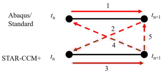
Figure 1.
The procedure for a single coupling step with implicit solvers.
3. Model Tests
3.1. Test Models and Test Point Arrangement
The research object of this test was a wedge. The wedge model was 600 mm long and 300 mm wide with a fixed aspect ratio. The shape of the bottom section of the model was V-shaped (wedge). The inclination angles of the bottom plate (β) were 10°, 20°, 30°, and 40°. The detailed dimensions of the two-dimensional wedge model are shown in Figure 2a.
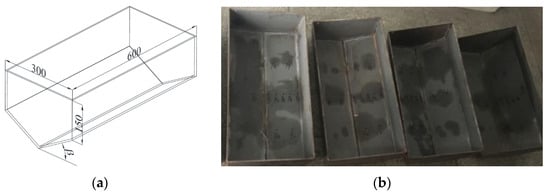
Figure 2.
Size of test models (Unit: mm). (a) model shape. (b) model with different deadrise angles.
In order to make the fluid flow two-dimensionally during the impact of the wedge into the water, the structure of the model remained unchanged in the length direction. In addition, as shown in Figure 2b, in order to give the structure a large buoyancy reserve after entering the water, the wedge-shaped structure was designed with vertical baffles added around it.
In order to measure the slamming pressure at different positions on the base plate of the test model, the measuring points were arranged at different height positions on the bottom plate, and the measuring points were compared to corresponding measuring points. The specific distribution of the wedge measuring points is shown in Figure 3. The center of the bottom plate (the angle of inclination with respect to the horizontal plane) was O point, and the measuring point P1 was arranged at a distance of 15 mm from the O center on the lateral centerline of the bottom plate and then one measuring point was arranged every 30 mm; that is, P2, P3, P4, P5, P6, and P7 in Figure 3a are the comparative measuring points of P2 and P4 in the horizontal direction (the other side of the bottom plate). P8, P10, P9, and P11 are the measurement points of P2 and P4 in the longitudinal direction for comparison. In addition, the openings in the bottom hole of test models and the fitting arrangement of pressure sensors are shown in Figure 3b.
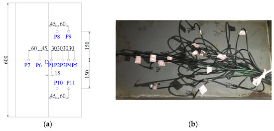
Figure 3.
Distribution and numbering of measure points on wedge bottom (Unit: mm). (a) Measure points on the wedge bottom. (b) Real scenery of pressure sensors.
3.2. Test Equipment and Devices
This test was carried out in a towing pool of the Jiangsu University of Science and Technology. The test piece model was suspended on the crane hook by a non-retractable steel cable. The initial drop height was determined by the crane lifting and the laser rangefinder (the determination of the test height was based on the distance from the lowest point of the test piece to the water surface). After adjusting to the specified height, the hook was released, and the test model was freely released into the water. In the test process, a high-speed camera photographed the test model’s release into the water. The signal acquisition system collected and recorded the test data measured by the pressure sensor through a wire. The test scenario for water entry of the structure is shown in Figure 4.
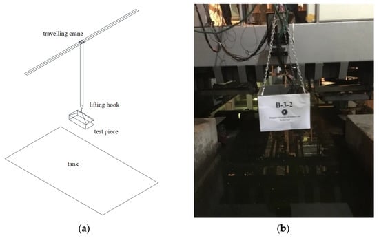
Figure 4.
Test scenario for water entry of structure. (a) Schematic diagram of the test scenario. (b) Actual test scenario.
The test acquisition equipment used during the test was as follows: (1) Laser rangefinder: measuring distance 750 mm, the sampling period was selected from 20/50/100/200/500/1000 μs, measuring accuracy was 2 μm; (2) High-speed camera: Model Phantom V12.1, sensor resolution was 1280 × 800, equipped with EDR dynamic range exposure control function and automatic exposure function, full-frame 1280 × 800, speed 6242 frames/second; (3) Pressure sensor: HM91 micro sensor and transmitter, the diameter was 6 mm, the sampling frequency was 10,000 Hz; (4) Dynamic signal acquisition system: two ruifeng real-time collectors, 48 channels, the sampling period was 0.5 microseconds.
During the processing of sample models, the thickness of the model steel plate was 5 mm. The quality and the corresponding number of each structural model after processing are given in Table 1. The initial height of water entry according to test conditions was determined to obtain the test cases. Each test condition was repeated three times.

Table 1.
Test cases for water entry of models.
3.3. Analysis of Test Results
According to the above test cases, the slamming test of the wedge-shaped structure was carried out to obtain the curve of the slamming pressure with time at each measurement point. In order to facilitate comparison and analysis, the time at which the test model was at a height of 0.01 m from the water surface was taken as the time 0.
3.3.1. Slamming Pressure at Different Deadrise Angles
Curves of slamming pressure at different measurement points on wedges with deadrise angles of 10°, 20°, 30°, and 40° over time are shown in Figure 5. It can be seen from the figure that the wedge with a deadrise angle of 10° (Figure 5a) reached the peak value of the slamming pressure immediately when it contacted the water surface. Over time, each measurement point had a significant peak value in succession and then rapidly decreased to a stable value, and the slamming pressure peaks at the measurement points P1 to P5 showed a trend of increasing first and then decreasing. In Figure 5b, the peak pressure of the slamming pressure at the measuring points P1 to P5 of the wedge with a deadrise angle of 20° also increased first and then decreased, but the position where the peak value of the maximum slamming pressure moved to the P2 measurement point. The peak slamming pressure of the wedges with deadrise angles of 30° (Figure 5c) and 40° (Figure 5d) gradually decreased from the measurement points P1 to P5. Unlike the first two types of wedges, the peak value of the maximum slamming pressure appeared at the P1 measurement point. This is mainly because when the wedge body enters the water, the bottom of the wedge with a small deadrise angle will cause a greater obstacle to liquid surface lifting, so the liquid surface continues to rise, and the squeezing force of the bottom plate on the liquid surface continues to increase, and the slamming pressure also increases continuously. After the liquid surface is lifted to a certain height, a jet phenomenon will occur, and the slamming pressure peak will appear at the root of the jet. After that, the jet is separated from the surface, and the slamming pressure decreases rapidly.
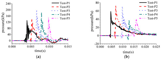
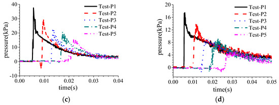
Figure 5.
Pressure of wedges with different deadrise angles β dropped from 0.4 m height. (a) = 10°. (b) = 20°. (c) = 30°. (d) = 40°.
Comparing the slamming pressure curves of Figure 5a–d, it can be found that the slamming pressure of the wedge changed with the change in the deadrise angle: the deadrise angle increased, and the slamming pressure decreased significantly. This is because the normal direction of the wedge force (the direction perpendicular to the surface of the wedge body) had a larger component when the wedge had a small deadrise angle, so the slamming pressure on the wedge was also significantly larger. In addition, the slamming pressure of wedges with different deadrise angles had different degrees of oscillation. When the deadrise angle was small, the oscillation frequency was low and the amplitude was large; when the deadrise angle was large, the oscillation frequency was high and the amplitude was small. This is because the difference in the deadrise angle resulted in changes in the amplitude and frequency of the shock wave. Table 2 shows the peak slamming pressure of the comparative measurement points of wedges with different deadrise angles and their occurrence time (due to the damage of the P7 measuring point during the test, individual data are not given). It can be found that the peak value of slamming pressure at the P2 and P4 measurement points and their comparative measurement points were almost the same by comparison. However, when the deadrise angle was 10° and 30°, the peaks value of the P6 and P7 measurement points appeared earlier than P2 and P4, and the peak value of the slamming pressure was too large. When the deadrise angle was 30°, the peaks value of P8 and P9 measurement points appeared later than P2 and P4, and the peak value of the slamming pressure was smaller. This is mainly because the wedges tilted at a small angle during the test, which resulted in the measuring points at the same height not entering the water at the same time, thus affecting the slamming pressure. However, since the wedge was tilted at an extremely small angle, the effect of test errors can be ignored.
Table 2.
Comparison of peak slamming pressure on contrastive measure points.
3.3.2. Slamming Pressure at Different Entry Speeds
Figure 6 shows the peak slamming pressure of the measurement points of the wedges at different deadrise angles at different drop heights. It can be seen from the figure that as the drop height increased, that is, the speed of entering the water increased, and the peak value of the slamming pressure also increased. However, the peak value of slamming pressure decreased as the deadrise angle increased for wedges with different deadrise angles falling from the same height.
Figure 6.
Peak pressure of the wedge with different water entry heights. (a) = 10°. (b) = 20°. (c) = 30°. (d) = 40°.
Comparing the measured points of the tip when the wedges with different deadrise angles had the maximum slamming pressure, it can be found that when the deadrise angle was 10°, the maximum slamming pressure tip appeared at the P3 measurement point and when the deadrise angle was 20°, the maximum slamming pressure appeared at the P2 measurement point. The maximum slamming pressure appeared at the P1 measurement point when the deadrise angle was 30° and 40°. The phenomenon is because when the deadrise angle was small, the liquid surface lift and the jet phenomenon had a greater effect on the peak value of the slamming pressure. When the deadrise angle was large, the peak value of the slamming pressure was hardly affected.
4. Simulation Analysis of a Wedge-Shaped Structure Slamming into Water
4.1. Verification of Numerical Methods
This section is mainly divided into two parts. The first is the comparison between the numerical model and the experiment result of water entry of a wedge. In this numerical model, the deformation effect of the structure was taken into account through the co-simulation of STAR-CCM+ and Abaqus. The other part is the comparison with the experimental results of the ship model in regular waves in reference [25]. In this part, in order to be more consistent with the experimental scene, the rigid body motion of the ship model was considered through the DFBI model.
4.1.1. Computational Model
The main scale parameters of the experimental model are shown in Table 3. The size of the overall calculated background area was 0.8 m × 0.8 m × 0.8 m, and that of the overlapping area was 0.4 m × 0.7 m × 0.35 m. The origin point of the coordinate system was at the midpoint of the wedge bottom, the Z axis was positive vertically, and the X axis was positive horizontally to the right, which satisfied the right-hand rectangular coordinate system, in which the height of the water surface was at Z = −0.01 m. For the setting of boundary conditions, the background area adopted the wall boundary condition, and the boundary condition of the top was the pressure outlet, the overlapping area of the wedge adopted the wall, and the rest adopted the overlapping mesh.
Table 3.
Principal dimension.
The origin of the coordinate system was at the intersection of the vertical line from the stern and the plane of the ship’s bottom. The X-axis pointed toward the bow along the length of the ship, and the Z-axis was perpendicular and pointed upward, satisfying the right-hand Cartesian coordinate system. The coordinates for the background domain area were [−8, −4, −4] and [24, 4, 4], while the overlapping region coordinates were [−1.5, −1.2, −0.5] and [5, 1.2, 0.8], as shown in Figure 7.
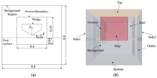
Figure 7.
Computational domain profile for simulation. (a) Computational domain for wedge. (b) Computational domain for ship.
The boundary condition settings for the background domain area and the overlapping region can be referred to in Table 4.
Table 4.
Boundary conditions of background and overset region in computational domain.
4.1.2. Grid Division and Time Step Setting
Due to the structure of the wedge involved the coupling of three-phase substances in the process of slamming, it was necessary to further track the large displacement movement of the structure and the free liquid surface, and the deformation of the structure made it necessary to reconstruct the mesh at each time step, which increased the complexity of calculation. To solve this problem, this paper introduced the three-dimensional overset mesh technology, which can consider the large deformation of the structure and is suitable for solving this kind of complex fluid–structure coupling problem without mesh reconstruction. In the computing area, the methods of surface reconstruction, the repair of the automatic surface, cutting mesh, and prismatic layer were used to generate meshes. In order to eliminate the errors caused by inserting variables between meshes, the same mesh density of the magnitude was used for the overlapping area of the background mesh and the overlapping mesh. See Figure 8a for the mesh division of the calculation area. The maximum mesh size was 0.02 m, the encrypted mesh size was 0.008 m, and the cutting body mesh unit was isotropic. There will be jet flow in the solid-liquid interface. In order to clearly capture the evolution form of jet flow, this chapter used mesh thinning technology to obtain fine mesh at the interface. The mesh density between the contact water surface and the wedge bottom is shown in Figure 8. The cutting body mesh unit was anisotropic. The mesh size near the water surface was 0.008 m in X and Y directions and the size in the Z direction was 0.008 m. The mesh size in X and Y directions in the falling area of the wedge bottom was 0.004 m. The mesh size of the overlapping mesh area was 0.004 m, and that of the V-shaped plate at the bottom of the wedge was 0.004 m.
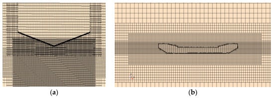
Figure 8.
Computational domain mesh. (a) Mesh density between water and wedge. (b) Mesh density between water and ship model.
In the process of numerical calculation, the Courant number c was used to balance the accuracy of calculation results and calculation efficiency. The Courant number indicates how many meshes have moved in the unit time step. After correct adjustment, the convergence can be accelerated, and the stability of the solution can be enhanced. The Courant number was 1 when first-order convection was used, and the Courant number was 0.5 when second-order convection was used. In this section, the time step was 2.0 × 10⁻⁶ s.
where is the time step length, is the mesh size, and is the wave velocity.
4.2. Calculation Results and Analysis
4.2.1. Comparison of Slamming Pressures for Wedges with Different Angles
The slamming values for wedges with different angles can be seen in Figure 9, which shows the slamming-pressure curve of a wedge falling from a height of 0.4 m. As can be seen from the graph, at an angle of 10°, the wedge (Figure 9a) had the highest slamming pressure when the slamming first occurred, with a large slamming pressure at the first measurement point on the wedge. Figure 9b shows a similar trend to that of the 10° wedge in terms of peak slamming pressure at measurement point P4 with an angle of 20, which also increased and then decreased. This is due to the fact that when the wedge dropped into the water, the bottom plate of wedges (10° and 20°) affected the water, so when the liquid level was continuously lifted, the free liquid surface was subjected to increasing squeezing pressure from the bottom plate, and therefore the slamming pressure also increased at this time. Once the free liquid surface rose to a certain height, wave breaking and peak of the slamming pressure appeared. This was followed by a gradual reduction in the slamming, which was caused by the separation of the wedge surface from the free liquid surface. And with the increase in the angle of the wedge, the rise in the free liquid surface was not affected too much by the base plate.
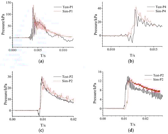
Figure 9.
Comparison of the predicted time history of pressure against experimental results for water entry of wedge with constant deadrise angle . (a) = 10° (b) = 20°. (c) = 30°. (d) = 40°.
As can be seen in Figure 9, the slamming pressure of the wedge changed as the angle of the wedge changed, and as the angle increased, the slamming pressure of the wedge decreased. A comparison of the values of the experimental and simulated values is shown in Table 5. As can be seen from the table, the results of the experimental and simulated values were close, with a small error rate of around 20%. The error in the results for the wedge of 10° was larger because the wedge was subjected to a higher air resistance, which was not considered in the numerical simulation.
Table 5.
Comparsion of simulation and experiment.
4.2.2. Comparison of Slamming Results for Different Heights of the Wedge
Figure 10 shows the comparison of the slamming pressure of the wedges at P1, P2, P3, and P4 for different velocities (different heights). The larger angle of the wedge indicated a lower pressure.
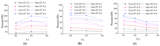
Figure 10.
Peak slamming pressure under different angles. (a) = 10° (b) = 20° (c) = 30°.
When the angle of the wedge was 10°, the wedge at the P3 had the highest slamming pressure value. When the angle of the wedge was 20°, the wedge at the P2 had the highest slamming pressure value. When the angle of the wedge was 30°, the wedge at the P1 had the highest slamming pressure value. This is because as the angle became smaller, the slamming pressure was influenced more by the rise in free liquid, and the wave-breaking phenomenon became more pronounced, while for wedges with a larger angle, the rise in free liquid and the wave-breaking phenomenon had relatively little effect on the slamming pressure.
In order to investigate the comparative slamming pressure of wedges at different water heights, comparative slamming pressure values are given in this section for wedges with a deadrise angle of 10° at 0.1, 0.2, 0.3, 0.4 m, for wedges with a deadrise angle of 20° at 0.1, 0.2, 0.4, 0.6 m, for wedges with a deadrise angle of 30° at 0.2, 0.4, 0.6, 0.8 m, and for wedges with a deadrise angle of 30° at 0.2, 0.4, 0.6, 0.8 m, respectively.
As can be seen from the graph, for the wedge of 10°, there was a certain error between the numerical simulation and the experimental peak slamming pressure, mainly because the wedge of 10° had a small angle and was susceptible to the influence of the jet when the liquid surface was lifted, so there was a certain error. For the wedges of 20° and 30°, the numerical simulations fit the experimental slamming pressure values better. Comparing the peak slamming pressures for wedges with different velocities at the same angle, it can be seen that the peak slamming pressure increased when the velocity became faster (the higher height).
4.2.3. Comparison of Slamming Results for the Ship Model
This section experiment investigated the slamming scenarios and structural response of an aluminum model ship under regular wave encountering conditions using a towing tank experiment. The experiments in the literature were conducted with 12 sets of calculations at velocities of 0, 1, and 1.5 m/s, wave frequencies of 0.56, 0.60, 0.64, 0.68, and 0.72 Hz, with wavelengths ranging from 3 m to 5 m. In this section, two sets of operating conditions (ship without speed and with speed) were selected for numerical simulation and compared with experimental results to validate the feasibility of the numerical method for wave-slamming response coupling in this section while analyzing the structural motion and slamming response characteristics. The selected two sets of operating conditions are shown in Table 6.
Table 6.
Two working conditions selected for simulation.
The comparison between the vertical loads at the connection point of the support strut and the hull obtained from numerical simulations of the aluminum model and the measured vertical forces on the support strut during experiments is shown in Figure 11. From the figure, it can be observed that the overall trend of the simulation results aligned well with the experimental values, with a high degree of agreement. However, the magnitude of the simulated loads was slightly lower than the experimental values. This could be attributed to the fact that wave experiments were conducted in a finite water tank where wall reflections of waves might have led to an overestimation of the experimental results. Additionally, the overall error for condition 1 was slightly higher than for condition 2, which could be due to the larger wave height in condition 1, resulting in a greater difference between the experimental and simulated values. Based on the load comparison curves in Figure 11, it can be concluded that the numerical simulation method proposed in this paper for the coupled response of the hull under wave slamming is effective.
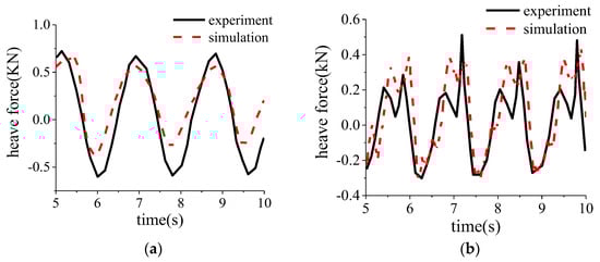
Figure 11.
Comparison of experimental and numerical values of heave force. (a) Work condition 1. (b) Work condition 2.
4.3. Effect of Structural Response for the Wedge
To analyze the effect of the inclined angle of the wedge bottom on the dynamic response of the wedge entering the water, the inclined angle of the wedge was varied to 10°, 20°, 30°, and 40°, with the wedge impacting the water surface at a speed of 10 m/s. The slamming pressure curves at points P1, P3–P5, for different inclined angles are shown in Figure 12. From the figure, it can be observed that except for the curve at an inclined angle of 10°, the curves for other angles of the wedge were similar. They all show that at the moment of contact between the wedge and the water surface, the slamming pressure quickly reached its peak. With time, the slamming pressure at each measuring point rapidly decreased after reaching a significant peak. A smaller inclined angle at the bottom resulted in a larger slamming pressure, consistent with the trend of changes in the maximum slamming pressure peak for different inclined angles, as shown in Figure 13. However, at an inclined angle of 10°, the slamming pressure reached its peak at the moment of contact between the wedge and the water surface, then quickly decreased, followed by a rapid rise and fall, forming periodic variations. Periodic fluctuations were also present at an inclined angle of 20° but with smaller amplitudes. This is due to changes in structural characteristics caused by variations in the inclined angle of the wedge bottom. A smaller inclined angle at the bottom resulted in a more violent water impact upon entry and made it more difficult for air to escape, leading to periodic changes in slamming force. Conversely, when the inclined angle was larger, water entry obstruction was reduced, resulting in lower slamming pressure and smoother slamming curves.
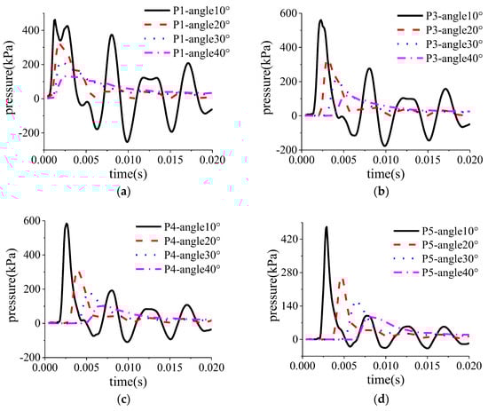
Figure 12.
Comparison of slamming pressure of each point with different angles. (a) P1. (b) P3. (c) P4. (d) P5.
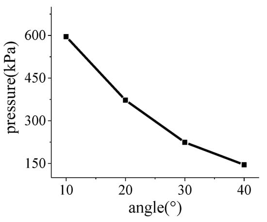
Figure 13.
Comparison of maximum slamming pressure peak values of wedges under different angles.
Figure 13 depicts the variation curve of the maximum pressure peak of the wedge with increasing bottom inclination angles while keeping the plate thickness (b = 5 mm), elastic modulus (E = 2.1 × 10¹¹ Pa), and water entry velocity (v = 10 m/s) constant. From the figure, it can be observed that as the bottom inclination angle increased, the maximum pressure value on the wedge gradually decreased. This is because increasing the bottom inclination angle reduced the obstruction to water entry for the structure, leading to a decrease in the slamming pressure experienced by the structure.
Figure 14a is the deformation displacement curve of measure points P1 to P5 on the wedge with a bottom deadrise angle of 10°. It can be seen from the figure that when the deadrise angle was 10°, the deformation displacement value of each measure point had a large fluctuation. Among them, P5 and other measure points had opposite phase differences. The closer the measuring point was to the bottom tip, the larger the deformation displacement and fluctuation. The smaller the bottom deadrise angle of the wedge, the greater the slamming pressure, the greater the deformation displacement, and the greater the fluctuation of pressure value and deformation value. Figure 14b is a comparison of the deformation displacement of P1 point on the wedge at different bottom deadrise angles. It can be seen from the figure that the curve fluctuated greatly when the deadrise angle was 10°, the displacement curves of each measuring point at other deadrise angles increased with time, and the smaller the deadrise angle, the larger the peak value of displacement. This is because when the bottom deadrise angle of the wedge was larger, the structure had fewer obstacles to enter water, but when the deadrise angle was smaller, the wedge was more affected by air coupling; not only did the slamming pressure increase but also deformation fluctuations occurred easily.
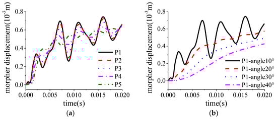
Figure 14.
Deformation displacement of each measuring point at different angles. (a) = 10°. (b) P1.
When plate thickness (b = 5 mm), modulus of elasticity (E = 2.1 × 10¹¹ Pa), and water velocity (v = 10 m/s) remained unchanged, the bottom deadrise angle increased. The change curve of the maximum deformation displacement of the wedge is shown in Figure 15. It can be seen from the figure that as the deadrise angle increased, the value of deformation displacement decreased continuously. This is because the larger the deadrise angle, the smaller the resistance to the structure, the smaller the deformation.
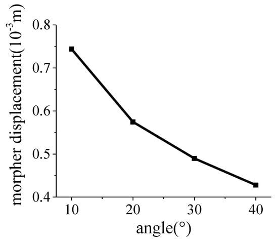
Figure 15.
Comparison of maximum deformation displacement under different angles.
Figure 16 shows the stress nephogram of a wedge with a deadrise angle of 10°and a thickness of 5 mm at different times. It can be seen from Figure 16a that when the wedge just touched the water surface, the maximum stress was concentrated at the tip of the wedge. It can be seen from Figure 16b,c that during the process of entering water, the stress concentration starts to shift upward from the bottom tip, and finally appeared in the center of the plate at the top of the wedge.
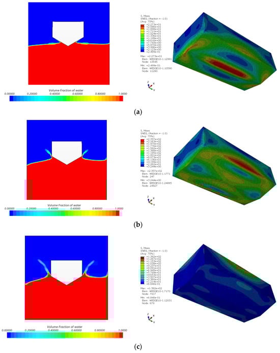
Figure 16.
Stress nephogram of a wedge with β = 10°and a thickness of 5 mm at different times. (a) t = 0.001 s. (b) t = 0.0022 s. (c) t = 0.0042 s.
4.4. Effect of Structural Response for the Ship Model
The Shape of the Free Surface and the Pressure Cloud Diagram at the Moment of Impact
Figure 17 illustrates the situation before and after the slamming of the aluminum model ship in condition 1. When the vessel floated on the waves, it experienced pitching and heaving motions due to the periodic fluctuations of the waves. From the figure, it can be observed that the bow of the ship tended to emerge from the water when it was positioned in a wave trough, and a relatively large relative impact occurred when the next wave crest arrived, leading to a slamming phenomenon. The figure mainly presents the shapes of the free surface of the model at different times and the pressure cloud diagram on the bottom surface of the ship. Figure 17a shows the shape of the free surface and the pressure cloud diagram on the model surface at t = 1.48 s. At this moment, the wave crest was located in the middle to aft position of the model, while the bow of the model was situated in a wave trough, with the bow surface completely emerging from the water. The bottom pressure was concentrated in the region of the bottom surface toward the stern, with the least pressure at the bow. Figure 17b indicates that at t = 2.06 s, the stern of the model was about to enter a wave trough, while the bow was positioned at the wave crest. The bow of the model was subjected to wave impact, and the bow surface of the model made full contact with the wave surface, with maximum pressure concentrated at the bow. Figure 17c shows that at t = 2.5 s, the wave crest had moved away from the bow toward the midship of the vessel, and the bow of the model gradually emerged from the water, with the maximum pressure concentrated in the front part of the ship’s bottom. During this condition, there were no significant surface deformations or wave-breaking phenomena on the wave surface.
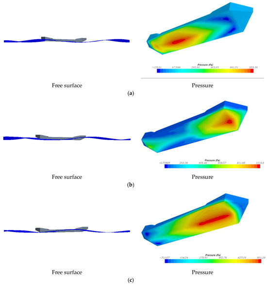
Figure 17.
The free surface elevation and the pressure distribution on the ship model at different times in the case 1. (a) t = 1.48 s. (b) t = 2.06 s. (c) t = 2.5 s.
As shown in Figure 18, a series of measurement points were arranged on the bottom of the ship to detect the slamming pressure and structural deformation displacement experienced by the ship in the waves. Point P1 was located at the top end of the bow, with coordinates (3.8, 0, 0.2). Points P2 and P3 were located at the bottom of the bow at the turning point, with coordinates (3.4, 0, 0) and (3.4, -0.2, 0.026), respectively. Point P4 was located at the bottom turning point of the stern, with coordinates (0.4, 0, 0).
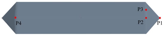
Figure 18.
Schematic map of measuring point position.
Figure 19 displays the pressure and velocity time history curves for different measurement points during condition 1. The solid lines represent the slamming pressure curves, while the dashed lines represent the velocity curves. The left Y-axis represents pressure values, while the right Y-axis represents velocity values. From Figure 19, it can be observed that both pressure and velocity curves exhibited periodic variations, reflecting the frequent occurrence of slamming loads. Additionally, it can be noted from the figure that the pressure amplitude at point P1 (top end of the bow) was the smallest, at 0.314 kPa, while the maximum pressure amplitude at point P2 (bottom of the bow) was 1.64 kPa. At point P3, it was 0.884 kPa, and at point P4 (bottom of the stern), it was 0.90 kPa. Slamming phenomena occurred successively at the bow and stern of the ship. The pressure curve peaks in the figure show some attenuation, possibly due to the viscosity and damping effects caused by the turbulence model, leading to wave height attenuation. Moreover, the pressure curve at point P2 exhibited a sinusoidal function form, consistent with the input of regular waves. At this point, the peaks of the slamming pressure curve and velocity curve corresponded, indicating the correlation between slamming load and slamming velocity. The pressure amplitude and velocity amplitude at the remaining points had certain phase differences. Except for point P1, the pressure curves at the other points were relatively regular. However, the pressure curve at point P1 exhibited a typical abrupt change characteristic of slamming pressure, with a certain stable region, which is related to the position of point P1 at the top end of the bow.
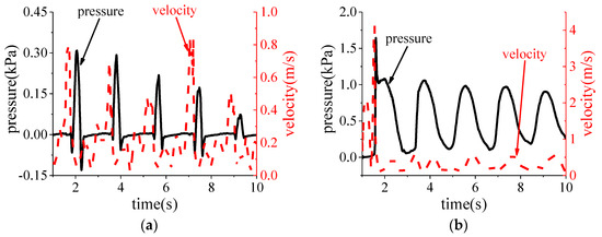
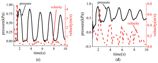
Figure 19.
Correlation curve of pressure and velocity at measuring point in case 1. (a) P1. (b) P2. (c) P3. (d) P4.
Figure 20 shows the stress (unit: MPa) and strain cloud diagram of the model structure at different times in condition 1.
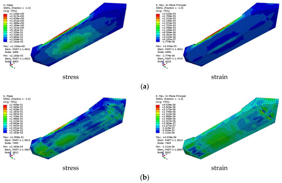
Figure 20.
Stress and strain nephogram. (a) t = 1.48 s. (b) t = 2.06 s.
Figure 20a depicts the stress and strain cloud diagram of the model at t = 1.48 s. As indicated in Figure 17 earlier, at t = 1.48 s, the aft part of the hull was positioned at the crest of the wave, while the bow was fully emerged from the water, resulting in midship bulging. This corresponds to large stress and strain concentrations at the bottom and sides of the hull in Figure 20a, while stress and strain were relatively lower at the bow. Figure 20b presents the stress and strain cloud diagram of the model at t = 2.06 s. At this moment, the waves impacted the inclined part of the model’s bow, leading to increased stress and strain in that region.
5. Conclusions
This study commenced with a series of controlled experiments, examining the impact of slamming on wedge-shaped bodies with varying inclinations from different heights. Following the empirical investigations, a comprehensive fluid–structure interaction (FSI) numerical model was developed. This model integrated the dynamic capabilities of STAR-CCM+ for fluid dynamics with the structural analysis power of Abaqus, considering the effects of structural deformations. To validate the accuracy and reliability of the numerical model, its predictions were compared with both the outcomes of the initial wedge-shaped body water entry experiments and existing data from ship-slamming studies under wave conditions. The model demonstrated high efficacy in replicating observed phenomena. Detailed analyses based on the experimental data from wedge-shaped bodies explored how slamming pressures varied with both the inclination angle and the water entry velocity (corresponding to different falling heights). The study yielded critical insights into slamming loads, free surface dynamics, structural deformations, and stress–strain responses under fluid–structure interaction conditions. The specific conclusions are as follows:
- (1)
- The factors predominantly influencing slamming pressure are the inclination angle and water entry velocity, which exhibit distinct impacts under varying conditions:
- (a)
- Inclination angle: For wedge-shaped bodies descending from a consistent height, an increase in the inclination angle results in a notable decrease in slamming pressure. At lower inclination angles, the dynamics of water surface lift-off and jet formation significantly alter both the location and intensity of the peak slamming pressure. In contrast, at higher inclination angles, the influences of lift-off and jetting on the peak slamming pressure are considerably diminished;
- (b)
- Water entry velocity: For structures with a constant inclination angle that impact the water surface from varying heights, the increase in falling height leads to a corresponding rise in water entry velocity. This elevation in velocity systematically amplifies the slamming pressure exerted on the structure. This relationship underscores the critical role of water entry velocity in determining the slamming impact, necessitating precise measurement and consideration in the analysis of fluid–structure interactions during high-velocity water entries.
- (2)
- The correlation between simulated and experimental slamming pressures was strong at inclination angles of 30° and 40°, demonstrating a high degree of model fidelity in these scenarios. However, at the lower inclination angles of 10° and 20°, discrepancies emerged between the simulated and observed peak slamming pressures. This deviation suggests that the current simulation might not adequately capture the dynamics of thinner water jets formed at these angles. To enhance the accuracy of the simulations at lower inclination angles, a refinement of the computational mesh is recommended. This adjustment would enable more precise modeling of the jet phenomena and improve the alignment between simulated and experimental results.
- (3)
- The relationship between the inclination angle of a wedge-shaped body and the resulting slamming pressure, structural deformation, and vibration susceptibility is inversely proportional. Specifically, a smaller inclination angle leads to an increase in slamming pressure, which, in turn, causes more substantial structural deformation and heightens the likelihood of vibration. At these lower inclination angles, the position and intensity of the slamming pressure peak are significantly impacted by phenomena such as water surface lift-off and jet formation. This observation underscores the critical influence of hydrodynamic behaviors on the structural response during water entry events, necessitating detailed consideration in both experimental setups and numerical simulations to ensure accurate predictions and robust structural design.
Author Contributions
Conceptualization, T.L. and X.Z.; methodology, T.L.; software, T.L.; Writing—original draft, T.L.; Writing—review and editing, J.W. and K.L.; Visualization, J.W. and K.L. All authors have read and agreed to the published version of the manuscript.
Funding
This research was funded by the National Natural Science Foundation of China (Grant No. 52171311; Grant 52271279) and the Open Project of the National Key Laboratory of Waterway Traffic Control (Grant No. W23CG090243).
Institutional Review Board Statement
Not applicable.
Informed Consent Statement
Not applicable.
Data Availability Statement
Data are contained within the article.
Conflicts of Interest
The authors declare no conflict of interest.
References
- Military in Metal Processing. The Shame of Japan’s Shipbuilding Industry-MOL COMFORT Shipbreaking Incident [EB/OL]. (2017-7-16). Available online: https://www.sohu.com/a/157626906_766672 (accessed on 3 March 2023).
- Yang, B. Study on Dynamic Response and Ultimate Strength of Container Ship Hull Structure under Slamming Loads. Ph.D. Thesis, Shanghai Jiao Tong University, Shanghai, China, 2019. [Google Scholar]
- Ochi, M. Prediction of slamming characteristics and hull responses for ship design. In Proceedings of the Annual Meeting of SNAME, New York, NY, USA, 15–17 November 1973. [Google Scholar]
- Yu, P.; Ren, H.; Li, C.; Liu, Y.C. Direct Calculation of Design Loads for Ship Bow Slamming. J. Ship Mech. 2016, 20, 566–573. [Google Scholar] [CrossRef]
- Hong, S.Y.; Kim, K.H.; Kim, B.W.; Kim, Y.S. Experimental Study on the Bow-Flare Slamming of a 10,000 TEU Containership. In Proceedings of the Twenty-Fourth International Ocean and Polar Engineering Conference, Busan, Republic of Korea, 15–20 June 2014. [Google Scholar]
- Hermundstad, O.A.; Moan, T. Numerical and experimental analysis of bow flare slamming on a Ro–Ro vessel in regular oblique waves. J. Mar. Sci. Technol. 2005, 10, 105–122. [Google Scholar] [CrossRef]
- Wang, S.; Guedes Soares, C. Experimental and numerical study on bottom slamming probability of a chemical tanker subjected to irregular waves. In Maritime Technology and Engineering; Taylor & Francis Group: London, UK, 2015; pp. 1065–1072. [Google Scholar]
- Lindemann, T.; Backhaus, E.; Ulbertus, A.; Oksina, A.; Kaeding, P. Investigations on the dynamic collapse behaviour of thin-walled structures and plate panels for shipbuilding applications. In Proceedings of the International Ocean and Polar Engineering Conference, Big Island, HI, USA, 21–26 June 2015. [Google Scholar]
- Wang, X.; Yang, P.; Gu, X.; Hu, J. Review of the theoretical investigation of slamming of global wave loads on ship structures. J. Ship Res. 2015, 10, 7–18. [Google Scholar]
- Wang, X.; Gu, X.; Hu, J. Springing investigation of a ship based on model tests and 3D hydroelastic theory. J. Ship Mech. 2012, 16, 915–925. [Google Scholar]
- Jiao, J.; Ren, H.; Sun, S.; Sun, L. Research on experimental technique of large-scale model under actual seaconditions. Shipbuild. China 2016, 57, 50–58. [Google Scholar]
- Zhu, R.; Lu, J.; Ji, R.; Xia, M.; Li, L.; Han, Z. Numerical Simulation of Three-Dimensional Wedge Entry Slamming under Wave Action. Ship Sci. Technol. 2019, 41, 6–11. [Google Scholar]
- Yang, B.; Wang, D. Dynamic Ultimate Hull Girder Strength Analysis on a Container Ship under Impact Bending Moments. Int. J. Offshore Polar Eng. 2018, 28, 105–111. [Google Scholar] [CrossRef]
- Mackie, A. The water entry problem. Q. J. Mech. Appl. Math. 1969, 22, 1–17. [Google Scholar] [CrossRef]
- Bilandi, R.N.; Jamei, S.; Roshan, F.; Azizi, M. Numerical simulation of vertical water impact of asymmetric wedges by using a finite volume method combined with a volume-of-fluid technique. Ocean Eng. 2018, 160, 119–131. [Google Scholar] [CrossRef]
- Bilandi, R.N.; Dashtimanesh, A.; Mancini, S.; Vitiello, L. Comparative study of experimental and CFD results for stepped planing hulls. Ocean Eng. 2023, 280, 114887. [Google Scholar] [CrossRef]
- Krastev, V.K.; Facci, A.L.; Ubertini, S. Asymmetric water impact of a two dimensional wedge: A systematic numerical study with transition to ventilating flow conditions. Ocean. Eng. 2018, 147, 386–398. [Google Scholar] [CrossRef]
- Zhao, Z. Research on Prediction of Slamming Pressure Load on VLCC Based on Two-Step Method. Ph.D. Thesis, Tianjin University, Tianjin, China, 2016. [Google Scholar]
- Zhang, B. Research on Strongly Nonlinear Slamming Loads of Ships Based on CFD Technology. Master’s Thesis, Dalian Maritime University, Dalian, China, 2020. [Google Scholar]
- Stavovy, A.B.; Chuang, S.-L. Analytical determination of slamming pressures for high-speed vehicles in waves. J. Ship Res. 1976, 20, 190–198. [Google Scholar] [CrossRef]
- Peng, D. Research on Dynamic Response of Ship Hull Structure under Slamming Loads. Master’s Thesis, Jiangsu University of Science and Technology, Zhenjiang, China, 2017. [Google Scholar]
- Wang, J.; Zhao, X.; Liu, K.; Hong, Z.; Zhou, T.; Jina, M. Local Area Linear Optimization of Large Cruise Ships Based on Wave Slamming Loads. Nav. Archit. Mar. Eng. 2022, 44, 55–62+123. [Google Scholar] [CrossRef]
- Chillemi, M.; Cucinotta, F.; Passeri, D.; Scappaticci, L.; Sfravara, F. CFD-Driven Shape Optimization of a Racing Motorcycle; Springer Nature: Cham, Switzerland, 2024. [Google Scholar]
- Lee, E.J.; Diez, M.; Harrison, E.L.; Jiang, M.J.; Snyder, L.A.; Powers, A.M.R.; Bay, R.J.; Serani, A.; Nadal, M.L.; Kubina, E.R.; et al. Experimental and computational fluid-structure interaction analysis and optimization of Deep-V planing-hull grillage panels subject to slamming loads—Part II: Irregular waves. Ocean Eng. 2024, 292, 116346. [Google Scholar] [CrossRef]
- Tuitman, J.T. Hydro-Elastic Response of Ship Structures to Slamming Induced Whipping. Ph.D. Thesis, Technische Universtiteit Delft, Delft, The Netherlands, 2010. [Google Scholar]
Disclaimer/Publisher’s Note: The statements, opinions and data contained in all publications are solely those of the individual author(s) and contributor(s) and not of MDPI and/or the editor(s). MDPI and/or the editor(s) disclaim responsibility for any injury to people or property resulting from any ideas, methods, instructions or products referred to in the content. |
© 2024 by the authors. Licensee MDPI, Basel, Switzerland. This article is an open access article distributed under the terms and conditions of the Creative Commons Attribution (CC BY) license (https://creativecommons.org/licenses/by/4.0/).