An Underwater Localization Algorithm for Airborne Moving Sound Sources Using Doppler Warping Transform

Abstract

When an airborne sound source is in rapid motion, the acoustic signal detected by the underwater sensor experiences a substantial Doppler shift. This shift is intricately linked to the motion parameters of the sound source. Analyzing the Doppler shift characteristics of received acoustic signals enables not only the estimation of target motion parameters but also the localization of the airborne sound source. Currently, the predominant methods for estimating parameters of uniformly moving targets are grounded in classical approaches. In this study, the application of the Doppler warping transform, traditionally applicable to sound sources in uniform linear motion, is extended to encompass a broader spectrum of sound source trajectories. Theoretical and experimental data validate the efficacy of this transform in linearizing the Doppler shift induced by a source in curved motion. Building upon this foundation, a methodology is proposed for locating airborne acoustic sources in curved motion from underwater. Sea experimental data corroborate the method’s effectiveness in achieving underwater localization of a helicopter target during curved motion.

1. Introduction

When an airborne sound source is in rapid motion, the acoustic signal received by an underwater receiver exhibits a significant Doppler shift. This shift exhibits a close correlation with the motion parameters of the source. Through the detection and analysis of the Doppler shift characteristics inherent in the received acoustic signals, we gain the capability to not only estimate the motion parameters of the target from an underwater perspective but also to pinpoint the precise location of the airborne sound source.

In the realm of existing technology, the estimation of motion parameters for airborne moving sources from underwater primarily relies on the classical method proposed by Ferguson, which focuses on estimating the parameters of a source in uniform linear motion using a single transducer [1,2,3,4]. Ferguson conducted extensive studies on the received acoustic signals of aircraft noise transmitted into the water, exploring their time-frequency and Doppler shift characteristics. Notably, the experiment successfully detected an airplane at a speed of 120 m/s from 4.6 km away in a deep-sea environment using a towed array. Conventional beamforming [5] (CBF) and minimum variance distortionless response beamforming [6] (MVDR) techniques were employed in these experiments to orient the airborne sources. Furthermore, Ferguson [7] introduced an algorithm for a single receiver to estimate the motion parameters of a target in uniform linear motion, leveraging the Doppler shift characteristics of the received signal fitted to the predicted values. Over the years, this method has been widely adopted to estimate the motion parameters of sound sources in uniform linear motion, demonstrating efficiency and accuracy in various application scenarios. Several enhanced methods have been proposed based on this foundational approach. To augment the accuracy of the extracted instantaneous frequencies, higher-order kernel functions have been introduced into time-frequency analysis [8,9,10,11]. Additionally, the parameter estimation algorithm has undergone refinement for diverse application environments [12,13], ensuring faster computation speed and more precise results.

The warping transform, initially introduced by Baraniuk et al. [14] in the context of signal processing, has found application in various fields. Bonnel et al. [15] were pioneers in applying the unitarily equivalent transform proposed by Baraniuk to the domain of underwater acoustics. They successfully transformed non-stationary dispersive signals, arising from the channel dispersion effect, into simpler quasi-single-frequency signals. This transformation facilitated diverse applications, including passive sound source detection [16,17,18].

The warping transform operates by resampling a complex non-stationary signal according to a functional relationship in either the time or frequency domain. Gao Deyang [19] introduced the Doppler warping transform and employed it in estimating the motion parameters of sound sources exhibiting uniform linear motion in the infinite free field. The Doppler warping transform serves as a valuable tool for addressing the nonlinear instantaneous phase problem associated with the Doppler shift. Linearizing this issue enables a more convenient estimation of motion parameters. However, it is noteworthy that the Doppler warping transform is specifically applicable to sources undergoing uniform linear motion in the infinite free field. Building upon this foundation, aiming at the coupling problem of the speed and the range at the closest point of approach, a motion parameter estimation method combining Doppler frequency shift and interference fringes and a method that combines modal interference and the Doppler shift carried by tonal signals was proposed by Sun Kai [20,21]. Considering a moving target radiating a broadband signal, Zhao Xiaojing [22] proposed a method of Doppler warping transform combined with the spectrum standard deviation to estimate the velocity of the target.

This paper presents a novel extension of the Doppler warping transform to encompass a broader spectrum of sound source motion paths and diverse sound field environments. This extension incorporates Doppler frequency shifts arising from the movement of sources along curved trajectories and the airborne excitation of sound fields underwater. Such innovation significantly augments the versatility of the method, rendering it applicable in more intricate and varied scenarios. We introduce a methodology for localizing airborne sound sources undergoing curved motion through the utilization of the extended Doppler warping transform. This advancement in the application of the transform holds promise for addressing challenges associated with complex motion paths, thereby expanding its utility in practical scenarios.

In this paper, after describing the theory of the Doppler warping transform, introducing the sea experiment, and extending the Doppler warping transform so that it is applicable to a target doing curved motion, a methodology for underwater localization of airborne moving sound source employing the extended Doppler warping transform is proposed. Then, the results of processing the sea experimental data using the proposed method are presented to validate the effectiveness of the method. The subsequent sections contain a discussion of the processing results and the conclusions of the whole paper.

2. Methods Introduction and Experiment

2.1. Theoretical Derivation

2.1.1. Doppler Frequency Shift Mode

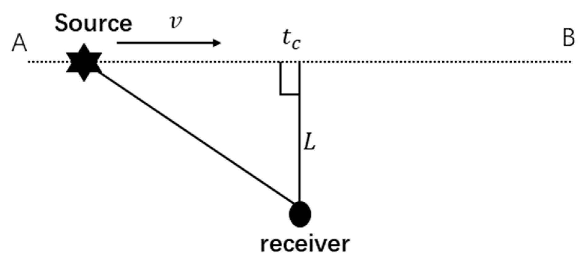
Figure 1 shows the infinite free field. The scenario assumes a stationary receiver and a sound source moving uniformly in a straight line from A to B at a speed of $v$, radiating a single-frequency signal. The nearest distance between the receiver and the source trajectory is $L$, and the speed of sound in the medium is $c$. The moment of arrival at the nearest point to the receiver is $t_c$.

In consideration of the scenario wherein the acoustic signal, emanating from a mobile source at time $\tau$, is subsequently received by the receiver at time $t$, the resultant distance between the receiver and the source is denoted as $r$.

$r$ can be calculated using the following geometric relationship:

$$r=c(t-\tau )=\sqrt{L^2+v^2{(\tau -t_c)}^2}$$

(1)

after rearrangement, we have:

$$(c^2-v^2){(\tau -t)}^2-2v^2(t-t_c)(\tau -t)-[L^2+v^2{(t-t_c)}^2]=0$$

(2)

solving the quadratic equation yields:

$$\tau -t=\frac{v^2(t-t_c)\pm \sqrt{L^2(c^2-v^2)+c^2{v}^2{(t-t_c)}^2}}{c^2-v^2}$$

(3)

Thus, it is possible to establish a functional relationship between $\tau$ and $t$. Considering that the moment of the signal from the sound source is always before the moment of the signal received by the receiver, there is $\tau <t$, so:

$$\tau (t)=\frac{c^{2}t-v^2{t}_c-\sqrt{L^2(c^2-v^2)+c^2{v}^2{(t-t_c)}^2}}{c^2-v^2},$$

(4)

At the instant $\tau$, the phase of the sound source vibration is:

$$\begin{array}{c}\varphi (t)=2\pi f_0\tau (t)+{\varphi }_0\\ \hspace{1em}\hspace{1em}\hspace{1em}\hspace{1em}\hspace{1em}\hspace{1em} \hspace{1em}\hspace{1em}\hspace{1em}\hspace{1em}=2\pi f_0\frac{c^{2}t-v^2{t}_c-\sqrt{L^2(c^2-v^2)+c^2{v}^2{(t-t_c)}^2}}{c^2-v^2}+{\varphi }_0\end{array}$$

(5)

In the context of the aforementioned scenario, let ${\varphi }_0$ represent the initial phase, and $t$ denote the moment when this vibrational phase $\varphi$ propagates to the receiver. The derivative of the phase with respect to time yields the frequency. Consequently, the instantaneous frequency received at the receiver can be expressed as follows:

$$\begin{array}{c}{f}_d(t)=\frac{1}{2\pi }\frac{d\varphi (t)}{dt}=\frac{f_0}{2\pi }\frac{d\tau (t)}{dt}\\ \hspace{1em}\hspace{1em}\hspace{1em}\hspace{1em}\hspace{1em}\hspace{1em}\hspace{1em} =f_0\frac{c^2}{c^2-v^2}\left[1-\frac{v^2(t-t_c)}{\sqrt{L^2(c^2-v^2)+c^2{v}^2{(t-t_c)}^2}}\right]\end{array},$$

(6)

In consideration of Equations (5) and (6), it becomes apparent that, despite the emission of a single-frequency signal by the sound source, the Doppler effect induced by its motion results in nonlinear variations in the instantaneous phase and frequency of the received signal over time. Consequently, the Doppler signal detected by the receiver exhibits non-stationary characteristics. The received signal can be mathematically expressed as:

$$\begin{array}{c}x(t)=A(\tau )\exp [-j(2\pi f_0\tau (t)+{\varphi }_0)]\\ \hspace{1em}\hspace{1em}\hspace{1em}\hspace{1em}\hspace{1em}\hspace{1em}\hspace{1em}\hspace{1em}\hspace{1em}=\frac{A_0}{r}\exp [-j(2\pi f_0\frac{c^{2}t-v^2{t}_c-\sqrt{L^2(c^2-v^2)+c^2{v}^2{(t-t_c)}^2}}{c^2-v^2}+{\varphi }_0)]\end{array},$$

(7)

where $x(t)$ denotes the acoustic signal radiated by a moving sound source at time $\tau$ received by the receiver at time $t$, where $A(\tau )$ is the amplitude, $f_0$ is the original frequency, ${\varphi }_0$ is the initial phase, and $A_0$ is the amplitude at the sound source.

2.1.2. Doppler Warping Transform Theory

In the work by Gao Deyang et al. [19], the Doppler warping transform operator is employed to linearize the instantaneous frequency of the line spectrum in a received signal originating from a uniformly moving linear source in a free field, as observed at a stationary receiver.

The concept of the warping transform, introduced by Baraniuk [14] in 1995, is a unitary equivalent transformation widely applied in signal processing. This technique accomplishes phase linearization by altering the time or frequency axis through a specific bijection relation. Assuming $x(t)$ represents the original signal, the general time domain warping transform process can be expressed as follows:

$$W_{h}x(t)=\sqrt{\left|h^{\prime }(t)\right|}x\left[h(t)\right],$$

(8)

The transformed signal $W_{h}x(t)$ is related to the original signal $x(t)$ through the warping transform operator $h(t)$, which is a bijection function. This means that each independent variable $t$ corresponds to a function value $h(t)$, and each function value $h(t)$ corresponds to an independent variable $t$. The warping transform is reversible and $\sqrt{\left|h^{\prime }(t)\right|}$ ensures that the energy before and after the transformation is conserved.

The warping transform is used to linearize the nonlinear Doppler line spectrum described in the previous section. The basic idea is to define the warping transform operator as the inverse function of $\tau$ to $t$, and to use the inverse function to achieve phase linearization with respect to the original function. Therefore, the following is an attempt to achieve phase linearization.

$$h(t)={\tau }^{-1}(t),$$

(9)

$$\begin{array}{ll}{\varphi }_D(t)& =\varphi [h(t)]=2\pi f_0\tau ({\tau }^{-1}(t))+{\varphi }_0\\ & =2\pi f_{0}t+{\varphi }_0\end{array},$$

(10)

The nonlinear Doppler phase variation with time generated by a source moving uniformly and linearly in a free field is shown in Equation (5). Since the instantaneous phase of the signal $\varphi (t)$ contains only the time-shifted component in $\tau (t)$, the functional relationship between $\tau$ and $t$ can be obtained from Equation (1):

$$t=\tau +\frac{\sqrt{v^2{(\tau -t_c)}^2+L^2}}{c},$$

(11)

Defining the warping transform operator as the inverse function of $\tau$ to $t$, and substituting $\tau$ with $t$ in the aforementioned equation, can be articulated as the Doppler warping transformation operator denoted by $h(t)$.

$$h(t)={\tau }^{-1}(t)=t+\frac{\sqrt{v^2{(t-t_c)}^2+L^2}}{c},$$

(12)

After substituting the expression for the Doppler warping transform operator into the nonlinear Doppler phase Equation (5) and simplifying it, the following has been obtained:

$$\begin{array}{ll}{\varphi }_D(t)& =\varphi [h(t)]=2\pi f_0\frac{c^{2}h(t)-v^2{t}_c-\sqrt{L^2(c^2-v^2)+c^2{v}^2{(h(t)-t_c)}^2}}{c^2-v^2}+{\varphi }_0\\ & =\frac{2\pi f_0}{c^2-v^2}(c^2-v^2)t+{\varphi }_0\\ & =2\pi f_{0}t+{\varphi }_0\end{array},$$

(13)

It is evident that the transformed signal achieves phase linearization after nonlinear resampling of the original signal using the Doppler warping transform operator. Additionally, the instantaneous frequency, which was nonlinearly transformed with time before the transformation, is restored to the original frequency of the sound source when it is stationary after the transformation.

2.1.3. Extended Doppler Warping Transform

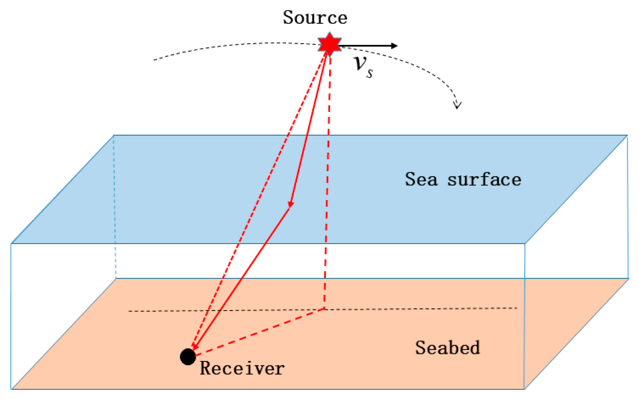
The Doppler warping transform operator discussed earlier is specifically applicable to a uniformly moving linear source in a free field. The subsequent objective is to extend the Doppler warping transform to linearize the Doppler nonlinear phase induced by an airborne curvilinear moving source at an underwater receiver. As depicted in Figure 2, an airborne sound source traverses a general curve. It is assumed that the source emits a single-frequency signal, and only the direct path of sound is taken into consideration. This sound wave propagates into the water, undergoes refraction by seawater, and ultimately reaches the receiver located at a depth of $d$.

Similar to the previous section, the underwater received acoustic signal can be represented as Equation (7). The Doppler warping transform is generalized to linearize the Doppler nonlinear instantaneous phase generated by a curved motion source, and the basic idea is still to define the warping transform operator as the inverse function of $\tau$ to $t$, and to use the inverse function to achieve the phase linearization with the relation between the inverse function and the original function, i.e., Equations (9) and (10).

However, unlike the analytical expression for the Doppler warping transform operator in free space, there is no specific analytical expression here. The relationship between $\tau$ and $t$ is demonstrated below:

$$t-\tau =T[L(\tau ),H(\tau )],$$

(14)

The variables $L(\tau )$ and $H(\tau )$ denote the horizontal distance and height of the sound source at time $\tau$, respectively. The time delay, represented by $T[L(\tau ),H(\tau )]$, corresponds to the duration it takes for the direct sound ray from the sound source, considering the horizontal distance $L(\tau )$ and the height $H(\tau )$, to reach the receiver. The time delay $T[L(\tau ),H(\tau )]$ can be calculated using the following formula [23]:

$$T[L(\tau ),H(\tau )]=\frac{1}{c[-H(\tau )]}[{\displaystyle {\int }_{-H(\tau )}^0\frac{n^2(z)}{\sqrt{n^2(z)-{\cos }^2\alpha }}dz}+{\displaystyle {\int }_0^d\frac{n^2(z)}{\sqrt{n^2(z)-{\cos }^2\alpha }}dz}],$$

(15)

Consider the sound speed profile in air, where the depth $z<0$ is in air, $z>0$ is underwater, $c[-H(\tau )]$ is the speed of sound at the source at the time $\tau$, $n(z)=c[-H(\tau )]/c(z)$ is the refractive index, and $\alpha$ is the swept angle of the outgoing sound line at the source, which satisfies the horizontal distance relation [23]:

$$L(\tau )=\cos \alpha [{\displaystyle {\int }_{-H(\tau )}^0\frac{1}{\sqrt{n^2(z)-{\cos }^2\alpha }}dz}+{\displaystyle {\int }_0^d\frac{1}{\sqrt{n^2(z)-{\cos }^2\alpha }}dz}],$$

(16)

Thus, the Doppler warping transform operator that linearizes the Doppler nonlinear phase generated by an airborne curvilinear motion source at an underwater receiver can be expressed as:

$$h(t)={\tau }^{-1}=t+T[L(t),H(t)],$$

(17)

The following section theoretically demonstrates that the operator mentioned above can convert the Doppler-shifted signal radiated by a curvilinear motion source into an approximate single-frequency signal. According to the theory of warping transform, after the warping transform operator $h(t)$ resamples the original signal nonlinearly in the time domain, the original signal will be transformed in the frequency domain as follows:

$$\stackrel{\sim }{f}=f{h}^{\prime }[h^{-1}(t)],$$

(18)

where $\stackrel{\sim }{f}$ is the frequency of the signal after warping, $f$ is the frequency of the signal before warping, and $h^{-1}(t)$ is the inverse function of $h(t)$. In order to make the derivation easy and clear, here we make $g(t)=h^{-1}(t)$, that is, we make $h^{\prime }[h^{-1}(t)]=h^{\prime }[g(t)]$. According to the chain rule of derivation, we have:

$$\frac{dh(g(t))}{dt}=h^{\prime }[g(t)]\frac{dg(t)}{dt},$$

(19)

So:

$$h^{\prime }[g(t)]=\frac{dh(g(t))}{dt}\frac{1}{\frac{dg(t)}{dt}},$$

(20)

namely:

$$h^{\prime }[h^{-1}(t)]=\frac{dh(h^{-1}(t))}{dt}\frac{1}{\frac{d{h}^{-1}(t)}{dt}}=\frac{dt}{dt}\frac{1}{\frac{d{h}^{-1}(t)}{dt}}=\frac{1}{\frac{d{h}^{-1}(t)}{dt}},$$

(21)

The Doppler frequency prior to the warping transform is essentially the derivative of the instantaneous phase (5) with respect to time:

$$f_d=\frac{1}{2\pi }\frac{d\varphi }{dt}=f_0\frac{d\tau (t)}{dt},$$

(22)

If the Doppler warping transformation operator is defined as in Equation (9), the transformed frequencies are

$$\stackrel{\sim }{f}=f{h}^{\prime }[h^{-1}(t)]=f\frac{1}{\frac{d{h}^{-1}(t)}{dt}}=f_d\frac{1}{\frac{d\tau (t)}{dt}}=f_0\frac{d\tau (t)}{dt}\frac{1}{\frac{d\tau (t)}{dt}}=f_0,$$

(23)

The above-derived Doppler warping transform operator can transform the Doppler frequency generated by a curvilinear moving source to the original frequency when the source is stationary.

2.2. Experiment

This section aims to validate the previously derived Doppler warping transform by applying it to actual sea experiment data, specifically focusing on transforming Doppler-shifted signals generated by a curved motion source into quasi-single-frequency signals. The experimental data utilized in this investigation originate from an underwater detection experiment targeting helicopters.

To provide clarity, a succinct introduction to the experimental scenario is presented. The experimental sea area exhibits an average water depth of approximately 94 m, characterized by a relatively flat seabed. In Figure 3a, the flight trajectory of the target helicopter is depicted. Departing from point X1, the helicopter proceeded in a straight line toward the southwest at an approximate speed of 49 m/s. It traversed the closest point to the receiving array on its way to point X2, where it arrived before executing a curvilinear motion for a certain distance. The entire process spanned approximately 10 min.

Figure 3b illustrates the altitude and velocity profiles of the helicopter, as documented by the onboard altimeter and GPS, over the course of the flight. Throughout the experiment, the helicopter was positioned farthest from the receiving array at point X1, maintaining a distance of approximately 16.8 km. At its closest point, the distance was reduced to approximately 3 km.

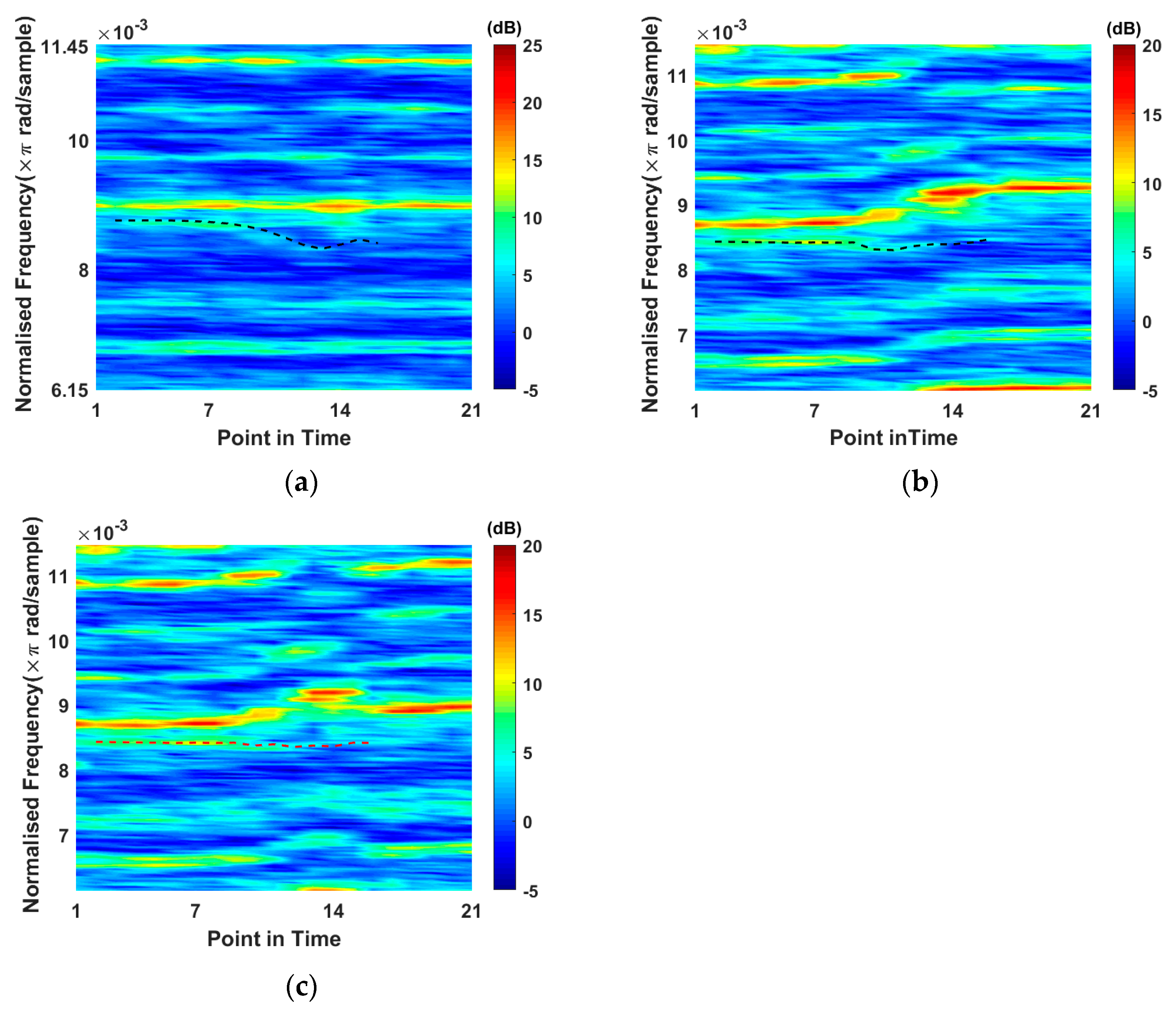
The received signals, with a total duration of approximately 10 min, are segmented into 21 segments with a 60% overlap rate between adjacent segments. The intermediate moments corresponding to these segments, denoted as the 1^st to 21^st time points, are considered. The time-frequency diagram of the received signal from the reference array element is presented in Figure 4a. The black dashed line in the figure represents the variation of the target line spectrum frequency over time, based on the position and speed records obtained from the helicopter GPS. In Figure 4b, the time-frequency diagram is depicted following the Doppler warping transformation, assuming the airborne helicopter follows a uniform linear flight path. The real speed of the helicopter, the nearest horizontal distance of the sound source from the receiver array, and the moment of reaching the nearest distance are substituted into the Doppler warping transformation operator. The black dashed line in the figure represents the transformed target line spectrum. Figure 4c illustrates the time-frequency diagram after the Doppler warping transformation without assuming a specific flight path for the airborne helicopter. Instead, the real horizontal distance and altitude at each instant are substituted into the Doppler warping transformation operator derived in this paper. This operator is designed to accommodate the curvilinear motion of the sound source. The red dashed line in the figure represents the target line spectrum after transformation.

According to the GPS records of the helicopter combined with the information presented in Figure 3a, the helicopter exhibited a nearly uniform linear flight trajectory from point X1 to point X2 during time points 1 to 15. Subsequently, the helicopter transitioned into a curvilinear flight pattern. Upon comparing Figure 4a to Figure 4c, it becomes evident that both Doppler warping transformation operators can induce a linearization effect on the instantaneous frequency of the original target line spectrum. This frequency variation is nonlinear over time during the phase of the target’s linear motion. Nevertheless, upon closer examination of the two transformation operators, it is observed that the transformed target line spectrum produced by the Doppler warping operator, assuming the airborne target is engaged in general curved motion, exhibits a more “straight” and linear profile during the curved motion phase of the target. This operator demonstrates superior capability in transforming Doppler-shifted signals generated by the moving target into quasi-single-frequency signals. The comparison suggests that the Doppler warping transform, applied under the assumption of general curved motion, effectively enhances the linearity of the transformed spectrum during the curved motion phase. This enhancement is crucial for transforming Doppler-shifted signals from a moving target into quasi-single-frequency signals. The results affirm the efficacy of the Doppler warping transform in converting Doppler-shifted signals generated by a moving sound source into quasi-single-frequency signals.

2.3. Estimation of Motion Parameters of a Sound Source in Uniform Linear Motion

This section provides a brief description of Ferguson’s method for estimating the motion parameters of a uniformly moving linear target using a single transducer.

As before, the instantaneous frequency $f_d(t)$ received by a stationary receiver at the $t$ moment when the source radiating a single-frequency signal is moving at a constant speed in a straight line can be expressed as:

$$f_d(t)=f_0\frac{c^2}{c^2-v^2}\left[1-\frac{v^2(t-t_c)}{\sqrt{L^2(c^2-v^2)+c^2{v}^2{(t-t_c)}^2}}\right],$$

(24)

Parametric transformations are applied to the above expressions:

$$\alpha \hspace{0.33em}=\hspace{0.33em}\frac{f_0{c}^2}{c^2-v^2},\hspace{0.33em}\hspace{0.33em}\hspace{0.33em}\beta \hspace{0.33em}=\hspace{0.33em}-\frac{f_{0}cv}{c^2-v^2},\hspace{0.33em}\hspace{0.33em}\hspace{0.33em}s\hspace{0.33em}=\hspace{0.33em}\frac{L\sqrt{c^2-v^2}}{vc},\hspace{0.33em}\hspace{0.33em}\hspace{0.33em}Z\left(t;t_c,s\right)\hspace{0.33em}=\hspace{0.33em}\frac{t-t_c}{\sqrt{s^2+{\left(t-t_c\right)}^2}},$$

(25)

Thus, Equation (24) can be written as:

$$f_d\left(t\right)\hspace{0.33em}\hspace{0.33em}=\hspace{0.33em}\hspace{0.33em}\alpha +\beta \cdot Z\left(t;t_c,s\right)\hspace{0.33em},$$

(26)

Then the general steps of the method proposed by Ferguson for estimating the motion parameters of a uniform linear target using a single sensor are as follows:

A time-frequency analysis of the signal from the receiving array element is performed to extract the target instantaneous frequency $g\left(t_j\right)$ at each moment $t_j\hspace{0.33em}\left(j=1,2,\cdots ,N\right)$ within the time period to be analyzed;

The following loss function is taken to estimate the parameter $\left\{t_c,\alpha ,\beta ,s\right\}$.

$$\begin{array}{ll}\left\{{\widehat{t}}_c,\widehat{\alpha },\widehat{\beta },\widehat{s}\right\}\hspace{0.33em}& =\hspace{0.33em}\arg \hspace{0.33em}\underset{t_c,\alpha ,\beta ,s}{\min }\left\{{\displaystyle \sum _{j=1}^N{\left[g\left(t_j\right)-f_d\left(t_j\right)\right]}^2}\right\}\\ & =\arg \hspace{0.33em}\underset{t_c,\alpha ,\beta ,s}{\min }\left\{{\displaystyle \sum _{j=1}^N{\left[g\left(t_j\right)-\alpha -\beta Z\left(t_j;t_c,s\right)\right]}^2}\right\}\end{array},$$

(27)

After estimating the parameter $\left\{t_c,\alpha ,\beta ,s\right\}$, the estimate of $\left\{t_c,f_0,v,L\right\}$ is obtained using the following equation:

$$\widehat{v}\hspace{0.33em}=\hspace{0.33em}-\frac{\widehat{\beta }\hspace{0.33em}}{\widehat{\alpha }}c,\hspace{0.33em}\hspace{0.33em}\hspace{0.33em}\hspace{0.33em}\hspace{0.33em}\widehat{L}\hspace{0.33em}=\hspace{0.33em}\frac{\widehat{s}\widehat{v}c}{\sqrt{c^2-{\widehat{v}}^2}},\hspace{0.33em}\hspace{0.33em}\hspace{0.33em}\hspace{0.33em}\hspace{0.33em}{\widehat{f}}_0\hspace{0.33em}=\hspace{0.33em}\widehat{\alpha }\left(1-\frac{{\widehat{v}}^2}{c^2}\right),$$

(28)

Assuming a scenario wherein the vertical separation between an airborne sound source and an underwater receiver is significantly smaller than their horizontal separation, it becomes feasible to approximate the airborne sound source as an underwater sound source. In this context, the height of the sound source is neglected in the consideration of the Doppler shift effect.

Furthermore, presuming a uniform linear motion of the airborne target along the horizontal direction, and employing the aforementioned approximation, we can employ a method to estimate the parameter $\left\{t_c,f_0,v,L\right\}$ through the above method. The estimation of the distance at various moments from the sound source can be derived from the formula $r\hspace{0.33em}=\hspace{0.33em}\sqrt{L^2+v^2{\left(t-t_c\right)}^2}$. This approach allows for a comprehensive analysis of the source–receiver distance at different instances during the sound transmission process.

The limitations of using Ferguson’s proposed method for estimating kinematic parameters and localization of an airborne source can be summarized as follows:

(1)

The airborne sound source needs to move uniformly in a horizontal direction, with the vertical distance between it and the underwater receiver being much smaller than the horizontal distance. This ensures that the effect of height is negligible.

(2)

The path of motion of the sound source should pass through the closest point to the receiving array. This is because it is where the instantaneous frequency change is fastest and has the most Doppler shift information.

(3)

The method hinges upon the extraction of target line spectrum points at discrete time intervals. This process necessitates a substantial Doppler shift in the received acoustic signal to ensure the inclusion of sufficient information regarding the motion parameters of the airborne sound source. In instances where the airborne sound source exhibits low frequency or slow movement, the resulting Doppler shift is small. Consequently, accurate estimations become challenging, particularly when the frequency resolution of the temporal analysis is constrained. Conversely, in scenarios characterized by a significant Doppler shift in the target line spectrum, the instantaneous frequency of the said spectrum undergoes nonlinear variations over time. This nonlinear behavior poses challenges in the tracking and extraction of the target line spectrum at each moment. The intricate interplay between Doppler shift magnitude and frequency dynamics underscores the complexity inherent in obtaining precise estimations, further compounded by limitations in frequency resolution during temporal analysis.

2.4. A Methodology for Underwater Localization of Airborne Moving Sound Source Employing the Extended Doppler Warping Transform

Addressing the aforementioned challenges, such as the limitation of Ferguson’s method to estimate parameters only for uniform linear target motion, this section introduces a method for localizing airborne moving sources from underwater. The proposed method leverages the Doppler warping transform, extending its applicability to airborne sound sources exhibiting general curvilinear motion.

The localization algorithm for airborne sound sources with general curvilinear motion employs the Doppler warping transform derived in the preceding section. The algorithm follows these general steps:

• The time-frequency diagram is constructed utilizing signals acquired from the reference array element. Subsequently, the line-spectrum extraction algorithm is employed for the identification of the line spectrum associated with the airborne moving target. This information is then integrated with the beamforming algorithm to derive the bearing-time records (BTR) of the target.
• Based on the bearing-time records of the airborne target, the beamformer dynamically adjusts its primary response direction at each time point to align precisely with the direction of the airborne target. Subsequently, spatial domain filtering is applied to the received signals at each time point, yielding spatial-filtered signals. Furthermore, LOFAR (low-frequency analysis and recording) spectrograms of these filtered signals are generated.
• Assuming that the vertical separation between the airborne source and the underwater receiver is significantly smaller than the horizontal distance between them, rendering the impact of height on the sound field negligible (with a known height denoted as $H$), an approach is adopted to reduce optimization calculations. The spatial-filtered signal is segmented into non-overlapping $N$ segments, with the middle horizontal distance of each segment designated as $\tilde{L}(t_j)\hspace{0.33em}\left(j=1,2,\cdots ,N\right)$. Subsequently, $\tilde{L}(t_j)\hspace{0.33em}$ is interpolated across the entire signal to obtain $\tilde{L}(t)$ at each moment. The interpolated horizontal distances at each moment are then incorporated into the Doppler warping transform operator ${\tilde{h}}_{mn}(t)=t+T_{mn}[\tilde{L}(t),H]$, tailored for the curvilinear movement of the source. This process is followed by a nonlinear resampling of the aforementioned spatial-filtered signal.
• The Doppler warping transformed signal is subsequently subjected to time-frequency analysis, and the line spectral point of the signal at the transformed time ${\tilde{t}}_j\hspace{0.33em}\left(j=1,2,\cdots ,N\right)$ is represented as $g\left({\tilde{t}}_j\right)$. Drawing upon the theory of the warping transform, a transitional relationship exists between the time point after the transform ${\tilde{t}}_j$ and the time point before the transform $t_j$, denoted as ${\tilde{t}}_j\hspace{0.33em}=h_{mn}^{-1}(t_j)$. A loss function is then formulated to estimate the horizontal distance $L(t_j)$ at each time point based on this transition relationship.

  $$\begin{array}{l}\left\{\begin{array}{c}\widehat{L}(t_j)=\underset{\hspace{0.33em}}{\arg \underset{L(t_j)}{\min }}\left\{{\displaystyle \sum _{j=1}^N{\left[g\left({\tilde{t}}_j\right)-f_0\right]}^2}\right\}\\ {\tilde{t}}_j\hspace{0.33em}={h^{-1}}_{mn}(t_j)\end{array}\right.\\ \hspace{0.33em}\hspace{0.33em}\hspace{0.33em}\hspace{0.33em}\hspace{0.33em}\hspace{0.33em}\hspace{0.33em}\hspace{0.33em}\hspace{0.33em}\end{array}$$

  (29)

That is, the closer the target frequency point of each moment after the transformation is to the original frequency when the sound source is stationary, and the more the instantaneous frequency of the transformed target line spectrum tends to change linearly with time, then it is considered to be more accurate for the horizontal distance of the sound source from the receiving array at each moment.

3. Results

Next, we employ data from a sea experiment to validate the efficacy of the aforementioned algorithm in localizing a curved motion sound source in the air. The array element data utilized in the previous underwater-to-air sound source detection experiment involving a helicopter as the target are still applied in this context.

Following the procedural steps outlined in this paper, Figure 4a depicts the time-frequency diagram of the received signal from the reference array element. The corresponding bearing-time records diagram is presented in Figure 5 below.

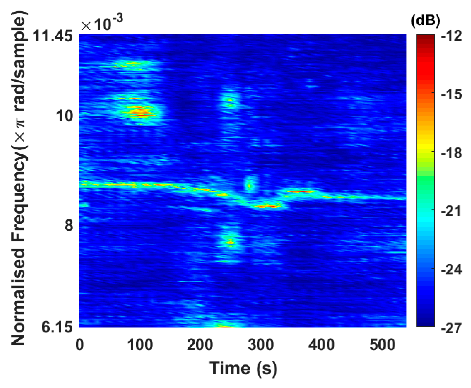
Considering the azimuthal trajectory of the designated target, the MVDR beamformer is employed to align the beam response direction with the identified target direction at each time instance. Subsequently, spatial domain filtering processing is applied, and the time-frequency analysis of the spatial domain filtered signal yields the LOFAR diagram of the helicopter target signal over an interval of approximately 550 s, as illustrated in Figure 6. This outcome aligns with prior analyses, indicating that the instantaneous frequency of the helicopter’s line spectrum undergoes notable nonlinear changes over time. Examination of the helicopter route diagram and the altitude and velocity versus time curves in Figure 3 reveals that the helicopter initially undergoes uniform linear motion for approximately 370 s, followed by a transition to a general curved motion.

As a comparison with the method proposed in this paper, the estimation of the motion parameters of the helicopter in roughly uniform linear motion for the first 370 s using the method proposed by Ferguson is shown in the following table (

Table 1. Results of motion parameters estimation.

	Moment of Arrival at the Nearest Point (s)	Source Speed (m/s)	Minimum Horizontal Range (m)
True value	337	49	3088
Estimated value	317.6	46.2	3154.7
Relative error	5.8%	5.8%	2.2%

).

In the proposed methodology, the entire 550 s signal is segmented into non-overlapping 10 s intervals. The midpoint of each segment serves as the time point for estimating the horizontal distance. Subsequently, the interpolated value is incorporated into the Doppler warping transform operator, specifically designed for the target curve motion. This facilitates the nonlinear resampling of the signal. The optimization process, as detailed in the preceding section, is then executed to determine the horizontal distance of the airborne source at different moments.

Following the optimization procedure outlined earlier, the horizontal distance of the airborne sound source is estimated at each time point. Figure 7a illustrates the LOFAR diagram obtained by nonlinearly resampling the signal using the motion parameters derived from Table 1 and the Doppler warping transform operator tailored for uniform linear motion. In Figure 7b, the LOFAR is depicted using the optimized horizontal distances for individual time points and the Doppler warping transform operator designed for general curved motion.

By comparing the LOFAR diagram depicted in Figure 7, it becomes evident that replacing the Doppler warping transform operator, designed exclusively for the uniform linear motion of the target, with the motion parameters estimated in Table 1, can only effectively restore the instantaneous frequency of the target’s line spectrum to its original frequency within the initial 370 s of its approximately uniform linear motion. However, deviations from the original frequency occur during the target’s curvilinear motion. By substituting the optimized horizontal distances for each time point into the Doppler warping transform operator, designed for general curved motion, the line spectrum’s instantaneous frequency of the target can be restored to its original frequency, maintaining accuracy throughout the motion of the target.

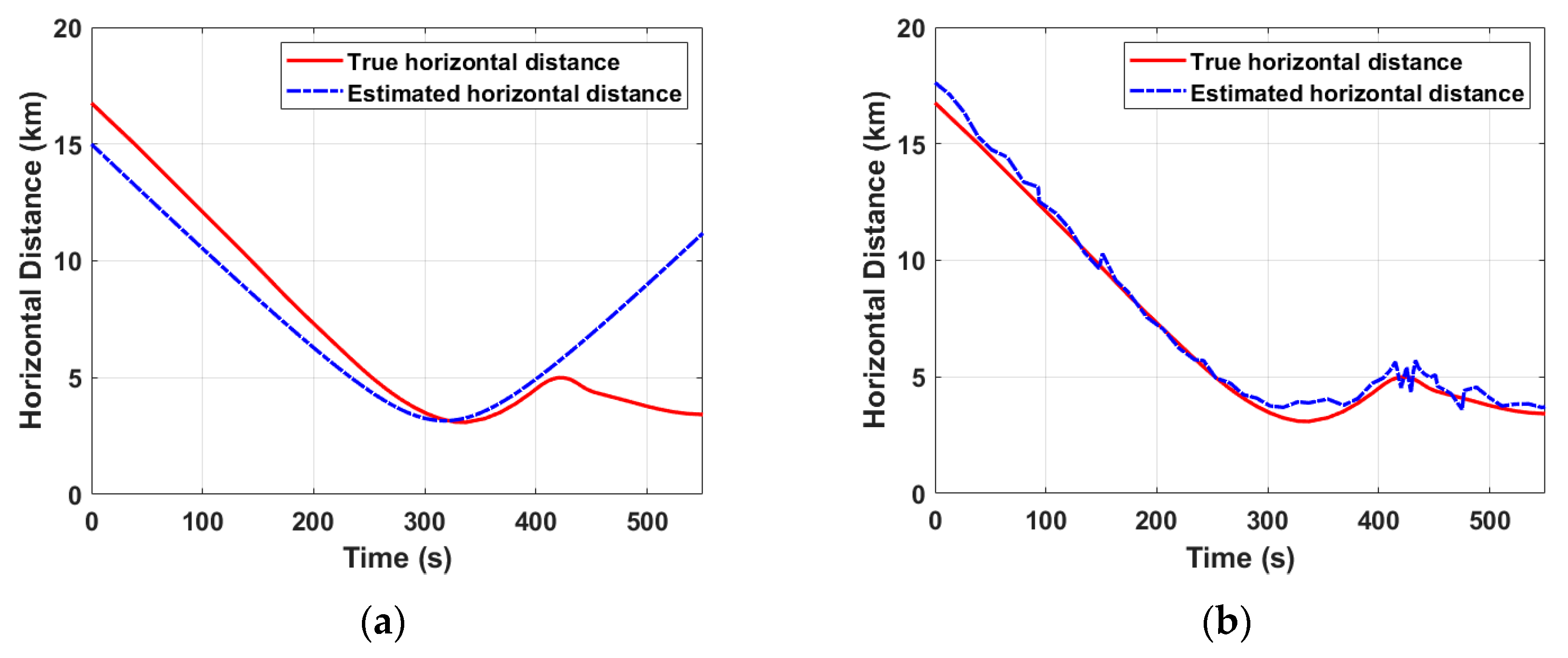
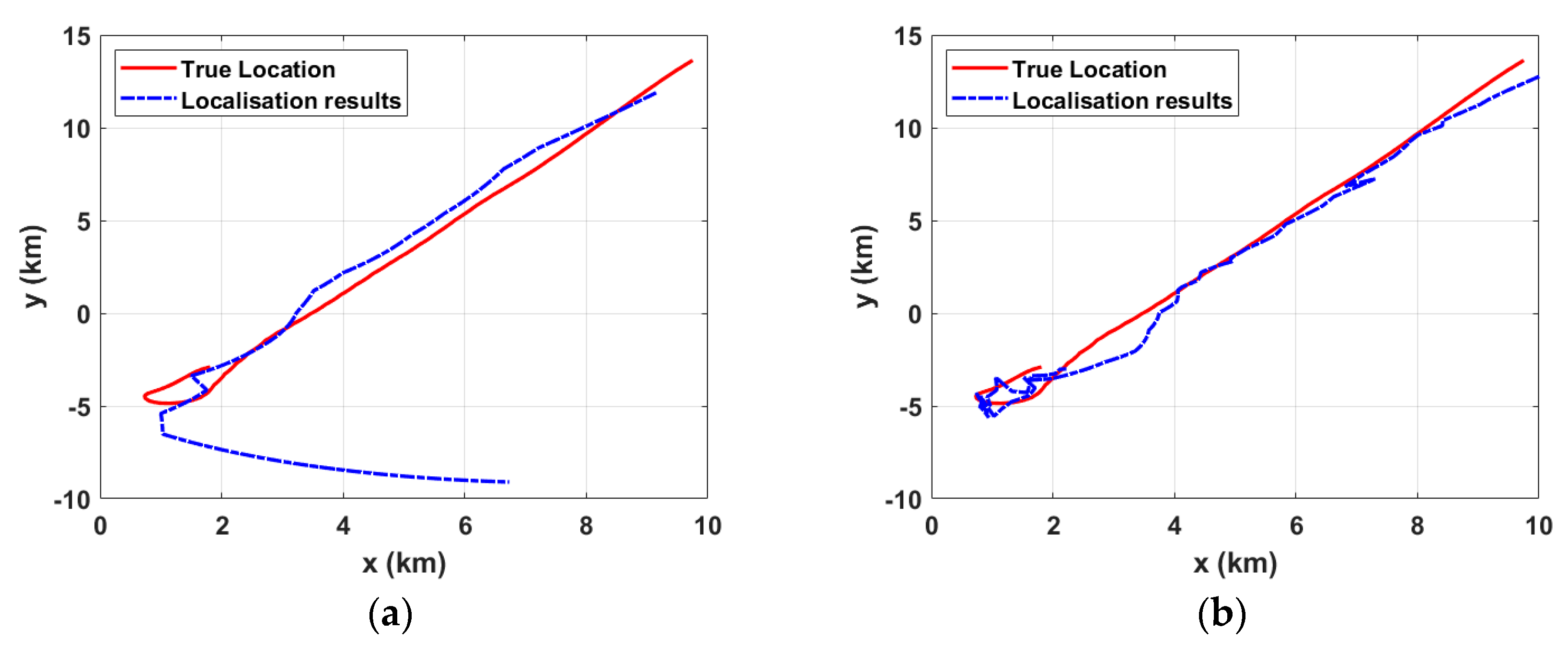
In Figure 8a, the horizontal distance between the sound source and the receiving array at each moment is illustrated after estimating the three motion parameters of $\left\{t_c,v,L\right\}$ using Ferguson’s proposed method and equation $r\hspace{0.33em}=\hspace{0.33em}\sqrt{L^2+v^2{\left(t-t_c\right)}^2}$. On the other hand, Figure 8b presents the estimated horizontal distance between the sound source and the receiving array at each moment using the method proposed in this paper. By amalgamating the results of horizontal distance estimation and the orientation estimation depicted in Figure 5, it becomes feasible to pinpoint the airborne sound source and estimate the position of the target, as demonstrated in Figure 9. It is noteworthy that the receiving array is situated at the origin of the coordinates.

4. Discussion

In the localization outcomes depicted in Figure 8 and Figure 9, it is evident that Ferguson’s proposed methodology exhibits only marginal errors in estimating horizontal distance and target position during the phase of straight-line motion. However, a noteworthy deviation from actual conditions arises when the target transitions into a curved trajectory. In contrast, our proposed approach not only adeptly localizes the target during straight-line motion but also demonstrates robust performance during curved motion. The localization results substantiate this, revealing an average error of 0.41 km in horizontal distance estimation.

5. Conclusions

The Doppler warping transform, previously confined to the uniform linear motion of sound sources, is generalized in this paper to linearize the Doppler nonlinear phase induced by curved motion sources. Its ability to convert the Doppler-shifted signal emitted by a curved motion source into an approximate single-frequency signal is demonstrated through theoretical derivation and sea-test data processing.

On this basis, a localization method for airborne sound sources in curvilinear motion is proposed, employing the generalized Doppler warping transform. Additionally, a comparison is introduced with the localization method put forth by Ferguson for airborne targets in uniform linear motion. Upon processing the sea experimental data from the underwater detection experiment involving the airborne sound source with the helicopter as the target, conclusive findings can be drawn.

• In contrast to Ferguson’s approach, the algorithm proposed in this study demonstrates the capability to track a target not only during uniform linear motion but also along curved trajectories. Experimental validation using data from sea trials attests to the effectiveness of the algorithm.
• Unlike Ferguson’s method, which necessitates the motion path of the sound source to pass the nearest point to the receiving array for enhanced Doppler shift information, our proposed method does not impose such a requirement. However, it still mandates sufficient Doppler shift information to uphold localization accuracy.
• The algorithm presented in this paper focuses on optimizing the horizontal distance at each time point, ensuring that the transformed instantaneous frequency closely aligns with the original frequency. Despite the necessity to optimize multiple parameters, the inter-independence of horizontal distance parameters at each time point results in a computationally efficient optimization process.

However, the method proposed in this paper exhibits certain limitations.

• The accuracy of localization may be compromised when the frequency resolution of the time-frequency analysis is low. This is particularly evident when the Doppler shift is reduced due to lower target line-spectrum frequencies and slower target motion, thereby impeding the acquisition of sufficient Doppler shift information.
• The present paper assumes that the target is situated in the far field, disregarding the influence of the sound source’s height on Doppler shift. In scenarios where the source is in close proximity to the receiver array, the impact of its height on the Doppler shift cannot be dismissed. Consequently, it becomes imperative to concurrently consider both the height and horizontal distance of the source and optimize them accordingly. Currently, a coupling phenomenon between the horizontal distance parameter and the height parameter occurs at each moment, leading to a degradation in the algorithm’s positioning performance and a significant increase in the computational requirements for parameter optimization.
• During the time-frequency analysis for data segmentation, the algorithm in this paper necessitates longer time data for each segment to enhance frequency resolution. This extended data requirement is crucial for obtaining sufficient line-spectrum Doppler shift features, thereby improving localization accuracy. However, this compromises the real-time processing capability of the algorithm.

Further refinements are essential to address these challenges.

References

- Ferguson, B.G. Doppler effect for sound emitted by a moving airborne source and received by acoustic sensors located above and below the sea surface. J. Acoust. Soc. Am. 1993, 94, 3244–3247. [Google Scholar] [CrossRef] [PubMed]
- Ferguson, B. Time-frequency signal analysis of hydrophone data. IEEE J. Ocean. Eng. 1996, 21, 537–544. [Google Scholar] [CrossRef]
- Ferguson, B.G.; Lo, K.W.; Speechley, G.C. Sensing the underwater sound field produced by a moving airborne signal source. In Proceedings of the OCEANS 2009-EUROPE, Bremen, Germany, 11–14 May 2009; pp. 1–7. [Google Scholar]
- Ferguson, B.G.; Speechley, G.C. Acoustic detection and localization of a turboprop aircraft by an array of hydrophones towed below the sea surface. IEEE J. Ocean. Eng. 2009, 34, 75–82. [Google Scholar] [CrossRef]
- Krim, H.; Viberg, M. Two decades of array signal processing research: The parametric approach. IEEE Signal Process. Mag. 1996, 13, 67–94. [Google Scholar] [CrossRef]
- Capon, J. High-Resolution Frequency-Wavenumber Spectrum Analysis. Proc. IEEE 1969, 57, 1408–1418. [Google Scholar] [CrossRef]
- Ferguson, B.G.; Quinn, B.G. Application of the short-time Fourier transform and the Wigner–Ville distribution to the acoustic localization of aircraft. J. Acoust. Soc. Am. 1994, 96, 821–827. [Google Scholar] [CrossRef]
- Reid, D.C.; Zoubir, A.M.; Boashash, B. Aircraft flight parameter estimation based on passive acoustic techniques using the polynomial Wigner–Ville distribution. J. Acoust. Soc. Am. 1997, 102, 207–223. [Google Scholar] [CrossRef]
- Valiere, J.-C.; Poisson, F.; Depollier, C.; Simon, L. High-speed moving source analysis using chirplets. IEEE Signal Process. Lett. 1999, 6, 113–115. [Google Scholar] [CrossRef]
- Xu, L.; Yang, Y.; Yu, S. Analysis of moving source characteristics using polynomial chirplet transform. J. Acoust. Soc. Am. 2015, 137, EL320–EL326. [Google Scholar] [CrossRef] [PubMed]
- Liang, N.; Yang, Y.; Guo, X. Doppler chirplet transform for the velocity estimation of a fast moving acoustic source of discrete tones. J. Acoust. Soc. Am. 2019, 145, EL34–EL38. [Google Scholar] [CrossRef] [PubMed]
- Quinn, B.G. Doppler speed and range estimation using frequency and amplitude estimates. J. Acoust. Soc. Am. 1995, 98, 2560–2566. [Google Scholar] [CrossRef]
- Timlelt, H.; Remram, Y.; Belouchrani, A. Closed-form solution to motion parameter estimation of an acoustic source exploiting Doppler effect. Digit. Signal Process. 2017, 63, 35–43. [Google Scholar] [CrossRef]
- Baraniuk, R.; Jones, D. Unitary equivalence: A new twist on signal processing. IEEE Trans. Signal Process. 1995, 43, 2269–2282. [Google Scholar] [CrossRef]
- Bonnel, J.; Thode, A.; Wright, D.; Chapman, R. Nonlinear time-warping made simple: A step-by-step tutorial on underwater acoustic modal separation with a single hydrophone. J. Acoust. Soc. Am. 2020, 147, 1897–1926. [Google Scholar] [CrossRef] [PubMed]
- Le Touze, G.; Torras, J.; Nicolas, B.; Mars, J. Source localization on a single hydrophone. In Proceedings of the OCEANS 2008, Quebec City, QC, Canada, 15–18 September 2008; pp. 1–6. [Google Scholar]
- Bonnel, J.; Dosso, S.E.; Chapman, N.R. Bayesian geoacoustic inversion of single hydrophone light bulb data using warping dispersion analysis. J. Acoust. Soc. Am. 2013, 134, 120–130. [Google Scholar] [CrossRef] [PubMed]
- Li, F.H.; Zhang, B.; Guo, Y.G. A Method of Measuring the In Situ Seafloor Sound Speed using Two Receivers with Warping Transformation. Chinese Phys. Lett. 2014, 31, 024301. [Google Scholar] [CrossRef]
- Gao, D.; Gao, D.; Chi, J.; Wang, L.; Song, W. Doppler-warping transform and its application to estimating acoustic target velocity. Acta Phys. Sin. 2021, 70, 124302. [Google Scholar] [CrossRef]
- Sun, K.; Gao, D.; Zhao, X.; Guo, D.; Song, W.; Li, Y. Estimation of target motion parameters from the tonal signals with a single hydrophone. Sensors 2023, 23, 6881. [Google Scholar] [CrossRef] [PubMed]
- Sun, K.; Gao, D.; Gao, D.; Song, W.; Li, X. Estimation of motion parameters of underwater acoustic targets by combining Doppler shift and interference spectrum. Acta Acust. 2023, 48, 50–59. [Google Scholar]
- Zhao, X.; Gao, D.; Li, X.; Song, W.; Li, Y.; Sun, K. Estimation of a moving broadband sound target motion velocity based on spectrum standard deviation. J. Sound Vib. 2023, 554, 117692. [Google Scholar] [CrossRef]
- Jensen, F.B.; Kuperman, W.A.; Porter, M.B.; Schmidt, H. Computational Ocean Acoustics, 2nd ed.; Springer: New York, NY, USA, 2011; pp. 196–198. [Google Scholar]