1. Introduction
With the widespread application of ocean engineering (such as in navigation systems [
1] or marine simulators [
2]), scientific visualization, film visual effects, video games, and other fields, the importance of real-time rendering of large-scale open sea scenes has significantly increased in recent years. The challenge at hand is to simulate and render large-scale ocean surfaces while maintaining a balance between efficiency and quality on power-limited platforms like web and mobile devices. Existing industrial solutions for addressing ocean surface rendering issues primarily involve techniques such as Fast Fourier Transform (FFT) for wave simulation [
3], which relies on bandwidth and general-purpose computing, Gerstner wave stacking technology [
4], which is constrained by iteration times, and the method of bump mapping [
5], which often lacks rendering details.
Eric Bruneton et al. proposed a GPU (Graphic Processing Unit) implementation of ocean rendering in their work [
6], which involves the analytical calculation of the normal of the ocean surface height field. They also introduced smooth filtering based on a hierarchical representation of mixing geometry. However, their method lacks dynamic filtering strategies for camera roaming, and the screen space strategy they employed faces challenges in handling changes in camera pose. In response to these limitations, we have implemented several improvements to address these issues. In our approach, considering the requirements for cross-platform compatibility, ease of deployment, and the need to balance performance and effectiveness in large-scale ocean surface rendering, we have designed a forward rendering solution without using the General-Purpose Graphics Processing Unit (GPGPU). This approach relies solely on the basic programmable graphics pipeline to avoid multiple passes and does not depend on any other specialized hardware extensions or compute shaders for non-graphics-related tasks. Additionally, we have utilized screen space level of detail and a self-adaptive filtering strategy to achieve a balance between performance and rendering quality. Our method offers advantages such as extremely low time cost and relatively high quality, making it suitable for applications in the field of ocean engineering.
Our main contributions are:
In
Section 3.2, we present a screen space level of detail strategy based on camera perspective and a novel adaptive filtering strategy based on virtual camera pose;
We propose a large-scale open sea surface modeling solution that does not rely on special hardware extensions. Our pipeline is lightweight and handy for deploying. It is described in detail in
Section 3.3;
We have increased the degree of freedom of virtual camera motion under the screen space strategy, as discussed in
Section 3.2.
A comparative analysis of our proposed method against four existing solutions in terms of efficiency has been conducted, specifically focusing on the time required for ocean surface height field modeling per frame. This comparison serves to highlight the advancements achieved through the implementation of our approach. Additionally, comprehensive tests have been performed to assess the modeling time cost at various camera heights, aiming to substantiate the efficacy of our level of detail and filtering strategy. The resulting renderings from different camera perspectives further underscore the enhanced degrees of freedom in camera movement facilitated by our methodology. To validate the usability of our system, we administered system usability scale questionnaires, the outcomes of which provide empirical support for the user-friendliness of our system. Detailed descriptions of our experimental procedures and findings can be found in
Section 4.
3. Methodology
The schematic diagram in
Figure 1 illustrates the fundamental workflow of our methodology. The diagram is divided into two main sections. The left side delineates the tasks executed on the CPU host, encompassing the generation of wave data utilizing a spectrum formula [
27], computation of transformation matrices for subsequent GPU processing, incorporation of camera specifics, and initialization of essential global variables crucial for modeling and shading, such as lighting parameters and temporal settings. On the right side, we elucidate the modeling pipeline executed on the GPU device, which encompasses four primary components. Firstly, in
Section 3.1, we present the Gerstner wave model derived from the simplified Euler equation, serving as the theoretical foundation for our wave simulation approach. Secondly, we delve into the self-adaptive screen space mesh generation detailed in
Section 3.2, functioning within the vertex shader stage and tessellation control shader stage. Furthermore,
Section 3.3 represents the crux of our methodology, introducing an innovative screen space adaptive filtering strategy to render animated waves at varying levels of detail. Lastly, we offer a concise overview in
Section 3.4 outlining our shading strategy, which, while not the primary focus of our research, plays a pivotal role in ensuring the seamless operation of the entire system.
3.1. Wave Model
The wave model begins with the Euler Equations of an incompressible fluid:
where
represents the velocity field,
represents position,
t is time,
p represents hydrostatic pressure, and
represents external force.
can be represented as a gradient of some scalar field if it is conservative. In addition, for waves that have movements caused by a conservative force, we have
, and the velocity field
can be also represented as the gradient of some scalar function
where
represent field position. Furthermore, after linearization, if we assume
is just gravity, and consider only the changing shape of the water surface, this simplification allows us to neglect the complex ocean appearance such as surf breaking with bubbles; underwater motion can also be ignored. This focused approach enables us to derive the following simplified model:
Since we constrain wave movements on the ocean surface, we have
, where
is atmospheric pressure. After differentiating the first equation by
t, we obtain
. and by setting the kinematic term of surface
, we obtain:
By using bottom boundary conditions
in
and a free-surface boundary condition
in
to solve
[
28], we obtain:
In Equation (
4),
A denotes the amplitude,
represents the angular frequency, and
signifies the wave vector. As depth
, the velocity potential would be:
At the ocean surface, where
, the surface height field can be determined as follows:
To achieve the appearance of choppy waves in practical applications, it is advisable to introduce a slight offset along the gradient direction of the height field
, where
, as suggested by [
3]. Consequently, we have:
where
represents the offset of the horizontal projection of the ocean surface position
concerning the horizontal projection of field position
. Combining
and
, we obtain
. Therefore, the parametric equation for the ocean surface position
can be expressed as follows:
Equation (
8) demonstrates that the shape of waves can be effectively modeled using trochoids. Utilizing the Gerstner wave model
, it becomes straightforward to determine the height offset of each surface position relative to the horizontal plane
in world space. Additionally, this model facilitates the accurate calculation of the normal vector representation.
3.2. Self-Adapting Screen Space Meshing
In this section, our objective is to transform the wave model into a mesh representation. The desired outcome is to achieve the appearance of an infinite ocean surface from any viewpoint, provided that
and there is no roll component in the camera’s orientation (the treatment of the camera’s roll component is specifically addressed in
Section 3.2). Before proceeding, let us define some fundamental symbols:
denote the projection matrix and the camera view matrix, respectively; homogeneous coordinates
, with
, are used to represent a vertex point in screen space; and
is used to denote a mesh vertex in world space. Taking perspective division into account, the point at
along the
z-axis in world space can be depicted as follows:
Assuming
, namely the far clip plane distance of
is infinity, the projected position in NDC (Normalized Device Coordinate) space can be expressed as follows:
After perspective division, the
y component of
, denoted as
, represents the maximum height of the projected grid in screen space, as illustrated in
Figure 2b. To accommodate adaptive resolution, we leverage the hardware tessellation feature to tessellate the area of the screen that is occupied. Initially, we start with two patches comprising eight vertices
, which cover the screen’s NDC (Normalized Device Coordinates) area of
. Given that the camera motion lacks a roll component, the projected grid area must form a rectangle. Consequently, we can straightforwardly adjust the
y component of the four upper vertices of the two rectangles to
H.
We have prepared two rectangular patches for tessellation. To implement tessellation, we utilize OpenGL’s control shader and evaluation shader. A self-adaptive tessellation strategy is crucial to ensure that we do not generate an overly fine-grained mesh when the projected area is small. This situation often arises when the angle between the view direction and the
plane approaches zero. Let us define
N (with
dependent on the hardware device, typically
) as the subdivision count, which represents the maximum number of cells that can be subdivided along the width of the rectangle. The self-adaptive subdivision count can then be calculated as follows:
The OpenGL control shader plays a pivotal role in adjusting the tessellation level of detail within a quad domain by modifying its inner and outer levels. Following this, the evaluation stage of the pipeline subdivides the two patches into the desired triangle mesh. After tessellation, we obtain the positions of vertices
, each with a
z component of 0. The subsequent step involves implementing inverse projection to transform these vertices from NDC (Normalized Device Coordinates) space back to world space. Initially, it is important to note that the projected vertices
located on the far clip plane have a
z value of 1.
The direction vector from the camera position
to
should be:
The distance from
to the horizontal plane at
along
is represented as
.
So the intersection, namely inverse projected vertex position
can be represented as:
Following the application of inverse projection to all tessellated screen space triangles, they can be manipulated just like any conventional mesh.
Roll Component Processing
Euler angles are commonly used to represent rotations for rigid bodies in engineering practice due to their direct nature. Given a local coordinate basis
, it is straightforward to decompose a rotation into three components: pitch, roll, and yaw. These components describe the counterclockwise rotation, in radians, along each axis
. However, it is worth noting that Euler angles do not align with the convention adopted in ocean engineering and the marine sector in general [
29]. To address this, we can use Equation (
18) to facilitate the mutual conversion between Euler angles
and quaternions
. Additionally, in engineering practice, when
approaches
, we can adjust
by
to avoid the issue of gimbal lock.
As depicted in
Figure 2b, it is evident that the camera movement involving yaw and pitch components does not impact the horizontal orientation of the projection plane. Utilizing Euler angles, any arbitrary rotation matrix
in
can be expressed as:
Since matrix multiplication adheres to the associative law, we have the flexibility to postpone the roll component
until after the projected vertices’ offset, denoted as
, has been performed. This implies that we should separate
from the composite rotation matrix
.
Fortunately, in practice, our raw rotation data for camera movement is often represented by Euler angles or a quaternion rather than a rotation matrix. This means that
is readily available to us, and Equation (
20) is primarily for situations where Euler angles are not accessible to developers, such as in shader redevelopment. The final issue pertains to the local coordinate basis, which involves
describing the rotation by the base vector
, namely the forward vector of the camera. Consequently, the roll matrix should be computed using Rodrigues’ rotation formula:
where
represents the skew-symmetric matrix constructed by
.
should be calculated in the CPU host and then be transmitted into the GPU device as global data for proficiency consideration. We use Equations (
19) and (
20) to decompose roll component out of camera matrix
used in Algorithm 1 and the shading part, and we use Equation (
21) to construct
V used in
Section 3.2, Algorithms 1 and 2.
| Algorithm 1: Calculate Filter Threshold. |
Input: View direction , view matrix without roll component, camera position , distance n from camera to near clip plane, half fov , subdivision count N Output: Vertical length L for current grid cell - 1
calculate filter threshold; - 2
; - 3
; - 4
; - 5
; - 6
; // transform into camera space - 7
; // and in Figure 3 are equivalent- 8
; // and in Figure 3 are equivalent
- 9
; // transform back to world space - 10
; // transform back to world space - 11
; - 12
; - 13
; - 14
return L
|
Figure 3.
Algorithm for calculating vertical grid length of each screen space vertex.
Figure 3.
Algorithm for calculating vertical grid length of each screen space vertex.
| Algorithm 2: Meshing and Inverse Projection. |
![Jmse 12 00572 i001]() |
| Algorithm 3: Wave. |
![Jmse 12 00572 i002]() |
3.3. Screen Space Level of Detail
In the previous step, we obtained a flat triangle mesh plane, and the subsequent task is to displace each horizontal vertex by our wave model
. We must begin by generating wave data. A Gerstner wave is primarily composed of the following components: wavelength
, which represents the distance over which the wave completes one full cycle; amplitude
A, which denotes the maximum height of the wave; angular frequency
, which refers to the phase addition per unit time; and wave vector
, which describes the propagation direction of the wave. For optimization purposes, we generate these data [
30] using random number generators on the CPU host only once at the beginning and deliver it, along with any other shading-related data, to the GPU device memory through an OpenGL uniform buffer. This eliminates the need for updating to be performed during every render loop.
The Pierson–Moskowitz spectrum, based on measurements of waves taken by accelerometers on British weather ships in the North Atlantic, is utilized [
27]. The spectra are characterized by the following form:
which shows the energy distribution of gravity waves as a function of their frequency, where
,
,
and
is the wind speed at a height of 19.5 m above the sea surface, the height of the anemometers on the weather ships used by Pierson and Moskowitz in 1964 [
27].
Suppose we have
N waves with pre-calculated parameters, each animated vertex
will be offset by
. Consequently, we obtain the animated vertex as follows:
However, implementing this concept directly on our grid may not be ideal. This is because our screen-space projected grid is regular and uniform, resulting in significant variation in the resolution of the inversely projected horizontal grid for different
. In particular, the difference in the stride length that a grid represents between the camera’s near clip plane and far clip plane will be quite substantial. This discrepancy leads to a severe aliasing problem, as we attempt to sample waves across all frequencies with an irregular spatial sampling frequency, namely the inverse projected grid resolution. Low-pass filtering becomes essential. Given that we are using a free camera, the filtering strategy should be adaptive. We need to take into account the Nyquist sampling theorem:
in Equation (
24),
represents the sample frequency, and
denotes the maximum frequency of signal
s. If the sampling frequency is too low, it fails to accurately reconstruct the true signal; conversely, if the sampling frequency is excessively high, it results in a large frequency resolution. In practical scenarios, the sampling frequency is typically chosen to be higher than twice the Nyquist frequency (often by a factor of
k, where
). In our application, the sampling frequency, equivalent to the resolution of the inverse projected grid, remains fixed. To adhere to the Nyquist limit for each grid, we employ a low-pass filter for adaptation.
Back to physics, the mechanical wave parameter
represents the propagation length of the wave in a full phase,
represents the addition of phase per unit of time, and the wave speed
v can be represented as:
v indicates how far a wave propagates per unit of time, and when we fix time, we have a low-pass filter:
The illustration of our adaptive algorithm is shown as
Figure 3. Assuming we have a 2D camera atlas
,
L represent inverse projected grid length projected to
, the viewing direction unit vector. The intersection point
between
(which is equivalent to
in Algorithm 1) and screen space projected grid can be calculated by solving equation
for
.
Since the screen space projected grid is uniform, using
to represent the height of each screen space projected grid in world space, the offset of
along the top vector
can be represented as:
where
, and we can easily obtain an auxiliary vector
(which is equivalent to
in Algorithm 1).
In Algorithm 1,
shares the same principle as
t, and the threshold length
L can be calculated by:
The overall process of the modeling is shown in Algorithm 2, and the vertex attributes in the output of Algorithm 2 will be interpolated by the GPU for shading in the pixel shader.
3.4. Rendering
Since our focus is on modeling, we employ only fundamental shading techniques for rendering. This includes adopting a constant value for sun radiance and utilizing environmental mapping instead of atmospheric scattering models for global illumination.
Although the Algorithm 2 outputs interpolated vertex attributes to the pixel shader, including
,
,
, we can still follow the approach of [
6] to execute Algorithm 3 per pixel in the pixel shader, and we also follow the approach of [
6] to combine three different ways of dealing with the effects of the waves on scene appearance: displacement maps, normal perturbation, and BRDF (Bi-directional Reflection Distribution Function) modification with the help of the GLSL (OpenGL Shading Language) function smoothstep and the threshold
L. Although not as accurate as analytical calculations, in fact using attribute interpolation for coloring is still feasible. If interpolation is used for shading, more patches and vertices are needed to improve the grid resolution of screen space. At the same time, due to the issue of uniform grid resolution of screen space, certain hacks (such as volumetric fog) are needed to alleviate artifacts near the far clip plane.
Given the conversion of the filtering scale from grid to pixel, effectively resulting in an increased sampling rate, it is necessary for the filtering scale, denoted as
P, to be reduced:
The variable
h signifies the height resolution of the screen and
is the sampling frequency. Concurrently, given that the control flow on a GPU significantly depletes register resources, as highlighted in [
31], an optimization strategy is adopted from [
6,
31]. This approach involves pre-sorting the waves on the CPU host and employing a threshold
as the criterion for filtering levels. Subsequently, a mapping is utilized to directly ascertain the starting index, where
k represents the Nyquist sampling frequency.
where
C represents the size of the pre-sorted wave array. The visualization result of mapped indices is shown in
Figure 4b. It can be seen that as the
z value increases, the filtering interval continues to increase, which means that we can directly calculate the array interval instead of judging if
in Algorithm 3.
4. Results
We executed our system, developed in C++ and GLSL 4.5, on an Intel Core i5-12400F processor (Intel, Santa Clara, CA, USA) with 16 GB of memory (six cores) and an NVIDIA GeForce RTX 2060 GPU (NVIDIA, Santa Clara, CA, USA). Within this system, our core algorithms are integrated, and we will present our key findings in the subsequent sections.
To ensure a fair comparison, we exclusively focus on the time required for wave modeling and analytical normal calculation, both essential for shading purposes. Complex shading processes like atmospheric scattering or subsurface scattering are not taken into account in our evaluation.
With a
resolution and a camera height of 6 m, two quad patches, and maximum tessellation level
, using a NVIDIA Nsight Graphics tool to capture the frame, we obtain ≥1500 fps (disable v-sync) with 60 waves with
(1500 fps contains the time cost brought by the context of GLFW window form library and imgui GUI library). As described in
Section 3.4, we analytically calculate normals per pixel for shading. Since a large number of high-frequency waves are filtered out by low-pass filters in the modeling process, this gives a
ms time cost of the superposition of waves totally per frame, and when the camera height rises to 60 m, the total time cost of modeling and analytic normal calculating has been shrunk to
ms, and if we remove our self-adaptive filtering model, the time cost rises to close to
ms, no matter what camera height is selected, which proves our LOD strategy is effective. To verify the effectiveness of our self-adaptive filtering method and show its balance between performance and speed, we compare our algorithm with three current solutions: the built-in ocean water system of the Unreal 5 Engine based on Gerstner waves and a tile-based LOD system; NVIDIA WaveWorks 2.0 based on FFT and a Continuous Distance-Dependent LOD system; and a Quadtree tessellation LOD system.
To ensure the utmost fairness, after several tests, we used 100 waves in the Gerstner-wave-based method (ours, Unreal 5, Quadtree tessellation). As for the FFT-based method, known for its remarkable capabilities in simulating large-scale waveforms, WaveWorks 2.0, we adopted the configuration from NVIDIA’s official samples. The comparative outcomes are presented in
Table 1.
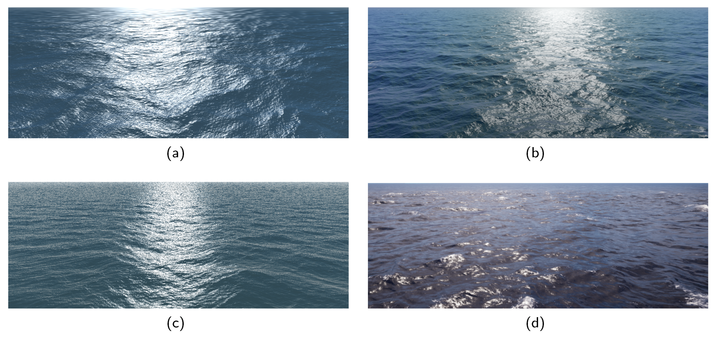
Figure 5 and
Table 1 present the visualization outcomes of four distinct methods. Within
Figure 5b, it becomes apparent that NVIDIA WaveWorks 2.0 stands out in terms of visual fidelity. Nonetheless, this superiority is offset by significant drawbacks, including elevated computation times on general-purpose hardware and intricate challenges in engineering execution, which collectively hinder its practical deployment. Furthermore, it necessitates additional multi-resolution FFT computations to fulfill anti-aliasing prerequisites, thereby exacerbating the IO load. As a result, FFT-based approaches find their niche primarily in high-end console or PC gaming environments, as well as in the realm of cinematic visual effects. Meanwhile, their application might not extend seamlessly to more resource-constrained platforms such as web applications and mobile games, or to specific use cases within ocean engineering, including navigation systems [
1] and marine simulation software [
2]. These considerations do not align with our present objectives.
In the Quadtree experiment, we utilized the traditional camera-position-based tessellation strategy for Level of Detail (LOD) purposes and calculated the normals analytically without applying any filtering to the model. The results are depicted in
Figure 5c. It is evident that as
, pixels near the horizontal line display significant aliasing issues. Unlike screen space tessellation, the irregularity and lack of uniformity in Quadtree nodes pose challenges in designing an effective low-pass filter. Additionally, rendering the ocean surface controlled by Quadtree nodes necessitates additional draw calls, resulting in increased time costs.
To corroborate the effectiveness of our method, we performed a series of tests aimed at assessing the rendering time required for a single frame across various camera heights
within a designated scene. In the interest of ensuring fairness, we contrasted these results with the time required to activate wind waves in WaveWorks 2.0, since the shading algorithm utilized by WaveWorks 2.0 demands a substantially higher computational effort in contrast to our approach. The results, depicted in
Figure 6, unequivocally demonstrate a decrease in rendering time cost as the camera height
y increases. This observation unequivocally underscores the efficiency of our Level of Detail (LOD) technique.
The results from the Unreal 5 experiment, illustrated in
Figure 5d, demonstrate a traditional ocean rendering pipeline that opts for interpolating geometry information within the fragment shader instead of utilizing analytic calculations. The grid near the horizon results in a discontinuous patchwork effect. Furthermore, this method capitalizes on high-quality textures crafted by artists to enhance visual expression. As a result, the specular component of the rendered ocean might not achieve the same level of realism when compared to alternative methodologies.
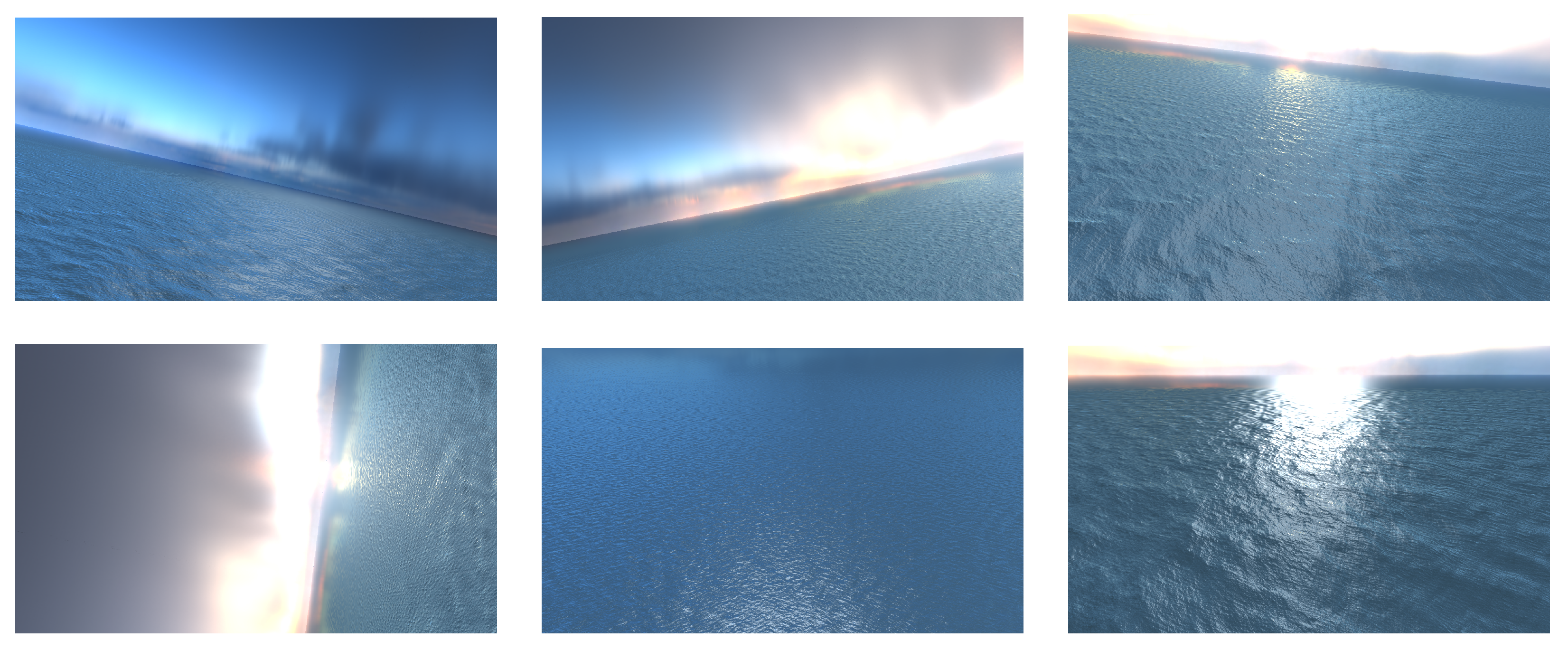
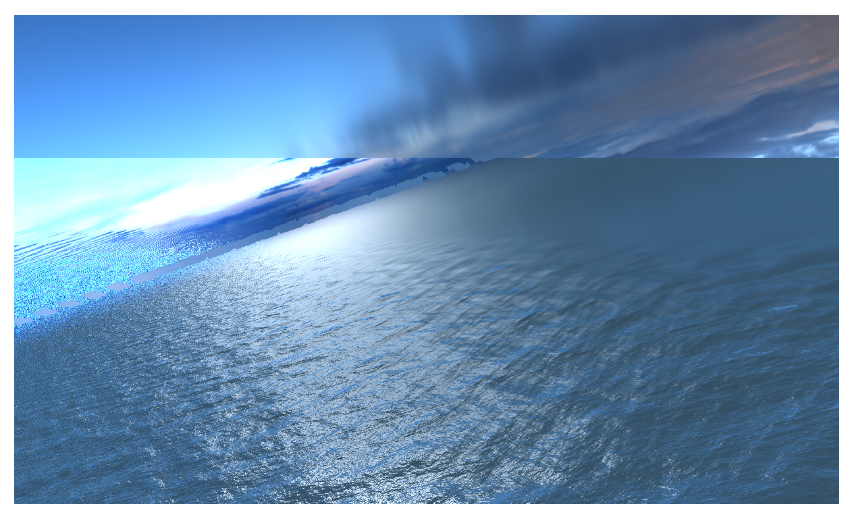
To substantiate the enhancement in the degrees of freedom for camera movement, we further selected camera viewpoints from varied perspectives for rendering. The outcomes derived are depicted in
Figure 7. Upon substituting
V with
as described in Algorithm 2, the issue arising from improper handling of roll components, as illustrated in
Figure 8 and further confirmed by the depiction in
Figure 2b, validates that our approach indeed amplifies the camera movement’s degrees of freedom without detriment to the screen space algorithm.
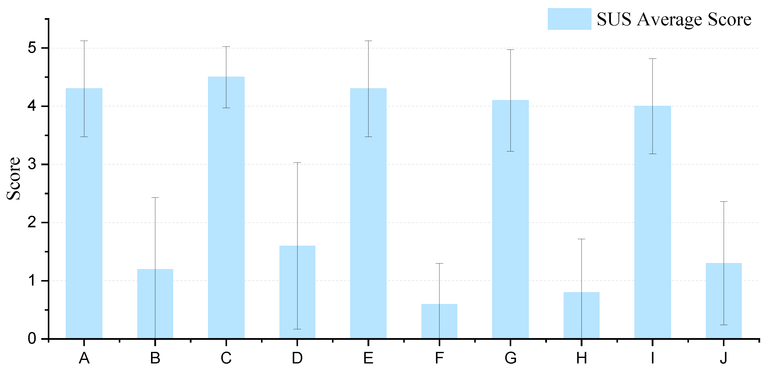
To evaluate the effectiveness of our method, we designed a questionnaire based on the System Usability Scale (SUS), encompassing the 10 questions presented in
Table 2. The ratings for each questionnaire range from 1 to 5. We invited 10 experts from relevant fields to interact with our system and complete the questionnaire. The scoring procedure for each question involves a transformation of the participant’s responses: for questions A, C, E, and G, the original score is reduced by 1, while for questions B, D, F, H, and J, it is subtracted from 5. These adjusted scores are then aggregated and multiplied by 2.5, converting the initial range of 0–40 to a standardized scale of 0–100. Based on research, a SUS score above 68 would be considered above average and anything below 68 is below average; however, the best way to interpret the scores is to produce a percentile ranking. The outcomes derived from the questionnaire are depicted in
Figure 9.
Although there are some disadvantages in appearance due to the use of a relatively simple shading algorithm, the results presented in
Table 1,
Figure 5, and
Table 2 do demonstrate that our approach outperforms the existing methods in terms of modeling efficiency. This superior performance can be attributed to the inherent benefits of utilizing screen space level of detail, where the granularity of primitives is determined by the screen resolution rather than the complexity of the scene itself. Concurrently, our novel self-adaptive filtering strategy adeptly addresses the challenge of non-uniform sampling across the projected grid. Moreover, in comparison to the FFT-based method, our approach of employing analytic calculations enables us to achieve competitive shading outcomes in simulations with a significantly reduced wave count.


