1. Introduction
Climate change and energy shortages are two rising issues on the agenda of the world. Human activities are driving the global warming trend observed since the mid-20th century, and the effects are irreversible and will worsen in the decades to come. Renewable energy sources, which are cleaner and more efficient, could play a pivotal role in sustainability development. The theoretical capacity of tidal energy in China reaches 110 GW [
1], indicating vast prospects for development. Its underwater generator, the tidal stream turbine (TST), does not occupy land resources, avoiding noise or visual pollution [
2,
3]. A TST can provide similar power to a bigger wind turbine [
4]. The above characteristics prove that tidal stream energy is attractive for electric power generation. However, TSTs are susceptible to factors such as biofouling [
5], sudden changes in instantaneous flow velocity [
6], seawater corrosion [
7], cavitation, and turbulence. These factors can result in mechanical faults or blade damage, leading to torque imbalances and voltage fluctuations, which significantly affect the quality of power generation, efficiency, and grid stability [
8,
9,
10]. Biofouling can cause an increase in device maintenance time and structural loading [
11]; there is also a biosecurity risk since immersed devices can serve as potential vectors for the introduction of non-native species [
12]. Therefore, timely and effectively detection of TST rotor attachment is of significant importance.
Current methods for TST rotor attachment detection primarily rely on electrical and image signals. Electrical signal-based methods, usually utilizing time–frequency or statistical analysis and machine learning, have shown some effect in detecting unbalanced rotor attachments [
13,
14,
15,
16]. However, these methods are susceptible to sea state and can find it difficult to detect balance attachments. Image-based methods overcome the shortcomings by analyzing the attachment conditions from underwater TST images directly. They focus on classification and semantic segmentation networks. Zheng et al. [
17] carried out attachment detection using an improved sparse autoencoder (SAE) and Softmax Regression (SR) method. They collected TST attachment images and divided the data based on the degree of attachment. Their proposed method achieved higher accuracy compared to the traditional principal component analysis (PCA) feature extraction algorithm. However, they only focused on TSTs in a static state, which is an idealized condition not reflective of reality. Therefore, Xin et al. [
18] collected TST images under operational conditions to make the dataset more representative of real-world scenarios. Then, the data were classified using a depthwise separable convolutional neural network (CNN), which achieved higher recognition accuracy than SAE+SR and a reasonable computational cost compared to large deep networks such as ResNet. However, the classification-based methods fail to precisely localize and display the biofouling. Peng et al. [
19] proposed a semantic segmentation network to identify TST blade attachments. It identified the TST blade edge by constructing two branches of coarse and fine segmentation. However, it requires a large number of labeled data, high computational costs, and a longer training time. Peng et al. [
20] proposed an image generation method, which extended and generated labeled data to reduce the workload of manual labeling. The proposed C-SegNet further improved the segmentation accuracy but performed poorly in contour localization. To address the localization misalignment caused by motion blur, Qi et al. [
21] combined preceding and succeeding frames for fault detection, significantly improving the localization accuracy on blurred images. However, a remaining challenge is the insufficient diversity in data, leading to inadequate network generalization. The limited data restricts data-driven algorithms to specific environments, posing a challenge for the application of TST attachment fault detection algorithms. Moreover, the severe degradation of underwater images will impact the extraction of features such as edges.
To address the above problem, this paper proposes a non-data-driven edge detection algorithm, Indexed Resemble-Normal-Line Guidance Detector (IRNLGD), for TST attachment fault detection. Focusing on the difficulty of extracting edge features in degraded underwater images, we employ an eight-directional gradient operator to extract image gradients. Next, to better utilize gradient direction information, we introduce the concept of “indexed resemble-normal line direction” and calibrate the gradient directions based on the trend of gradient changes. Finally, edge points are determined through the joint calibration of gradient direction and magnitude. The experimental results on the TST dataset and public datasets demonstrate IRNLGD’s effectiveness in dim images. What is more, a TST attachment fault detection method is explored on the basic of IRNLGD. A two-level detection is carried out with a data-driven lightweight classification network and the non-data-driven algorithm IRNLGD. It combines the advantages of both algorithms, providing more reliable and precise fault detection results.
The main contributions of this paper are as follows:
An effective edge detection algorithm, IRNLGD, is proposed to extract edge from low-contrast images.
A TST attachment fault detection method, MobileNet-IRNLGD, is explored, which combines data-driven and non-data-driven algorithms to strike a balance between limited data and precise detection.
The proposed TST attachment fault detection method is applied specifically to the real TST images, demonstrating the feasibility for engineering applications.
The remainder of the paper is organized as follows: In
Section 2, we review the related work on edge detection. In
Section 3, the proposed method is introduced in detail. Then, the experimental results and analysis are presented in
Section 4. Finally, we give the conclusions of this study in
Section 5.
3. Indexed Resemble-Normal-Line Guidance Detector
The edge detection algorithm proposed in this paper is divided into three steps: (1) The eight-direction gradients of the input image are calculated to form a gradient matrix. (2) The direction is calibrated according to the pairwise gradient magnitude, and the indexed resemble-normal-line direction is obtained according to the calibrated direction matrix. (3) The edge point determination is performed by combining the gradient magnitude and the indexed resemble-normal-line direction. In the following, we will introduce the proposed method in detail and return to its application in
Section 4.
3.1. Calculation of Eight-Direction Gradients
Gradients contain rich image information, and edge detection tasks can be performed using gradients. Traditional operators typically focus on two or four directions when computing gradients, thereby losing information from other directions. To obtain comprehensive multi-directional gradient information, an adjustable eight-direction gradient calculation method is proposed. The gradient magnitude for the first direction is calculated by
where
indicates the pixel intensity of the pixel
. We design an eight-directional gradient operator, sequentially rotating
from the first direction. According to Equation (
1), the eight-directional gradient operator is given by:
where
is the gradient amplification coefficient. It is introduced to amplify the gradient magnitudes without affecting subsequent gradient comparisons and direction calibration. Since the edge pixel intensity is based on the gradient magnitude, it is necessary to appropriately amplify the gradient values to enhance the edge. However, the calculation may overflow if
is too large. Here, we take
.
For the input image
, the gradient is obtained by convolution with the gradient operator in the corresponding direction. Therefore, according to Equation (
2), the gradient matrix can be written as
, where
Notice that . records pixelwise eight-direction gradient magnitudes of the input image, and the sequence indicates the corresponding direction. The gradient matrix provides the basic information for direction calibration and edge discrimination.
3.2. Indexed Resemble-Normal-Line Direction Calibration
In order to further utilize the cues of the gradient matrix, we introduce gradient directions in the form of recalibration. In classical algorithms, the role of gradient direction in edge detection tasks is to determine the edge direction and filter out pixels outside the specified direction. In this process, only the information of the maximum gradient direction or dominant direction is considered, resulting in the loss of information from other directions. Therefore, a novel gradient direction calibration method is proposed to preserve more useful cues.
According to the eight-directional gradients mentioned above, the calibrated direction is given by
where
is the calibrated direction matrix.
indicates the
calibrated direction of the pixel
.
consists of
, 0, and 1, indicating the change trend of a pixel spreading to its neighborhood. When the intensity increases, the corresponding direction is calibrated as 1.
More specifically, assume that there exists a neighborhood of size for pixel , and calculate the eight gradient magnitudes . The gradient direction calibration process is as follows:
Following the idea of obtaining multi-directional gradient information, the set of directions calibrated as 1 in
is defined as the indexed resemble-normal-line direction of the pixel
, marked as
, i.e.,
is an indefinite-length vector, with a length of . It contains the direction information of intensity growth. Different from traditional methods using single-direction information, the indexed resemble-normal-line direction records all directions where the intensity has an increasing trend. It preserves more gradient information and is beneficial for extracting edge features from degraded images. To fully utilize differential information across various directions, gradient magnitude and direction are retained to complement edge discrimination where gradient directions are not recorded in the indexed resemble-normal-line direction.
3.3. Edge Discrimination
Due to the characteristics of degraded underwater images, edge features such as gradients are suppressed. Traditional edge detection methods fail because they consider information limited to partial gradients in the image. Therefore, a multi-directional-based edge point determination method is proposed. The pixelwise edge discrimination is carried out by combining the gradient magnitude and the indexed resemble-normal-line direction. Inspired by classical Gestalt cues [
41]: similarity, continuity, and proximity, the following three criteria are proposed:
The gradient magnitude of the edge point is much larger than that of the non-edge.
The length of the indexed resemble-normal-line direction of the edge point satisfies .
Within neighborhood of the edge point, at least one pixel has the same indexed resemble-normal-line direction, and the gradient magnitude is about the same.
Criterion 1 follows the principle of abrupt changes in intensity at edges. The gradient reflects the intensity variation, where a larger gradient magnitude indicates a more significant grayscale variation and a higher likelihood of an edge. For criterion 1, the decision threshold is calculated as follows:
For the eight-direction gradient
of pixel
, the quadratic sum matrix
can be given as
To eliminate the effect of too small pixel values on the threshold calculation, a truncation parameter
is set, and a dynamic truncation threshold
can be obtained as
The pixel is involved if and only if its quadratic sum value is greater than
. Through experimental verification, here, we take
.
Then, the threshold
is calculated as
where
n is the number of pixels involved in the calculation.
Criterion 2 ensures that the detected edge points exhibit intensity variations in as many directions as possible. This helps in locating edge points accurately and also contributes to refining the edge. Criterion 3 aims to maintain edge continuity by controlling the similarity of gradients among neighboring pixels.
In conclusion, the proposed IRNLGD is finally detailed through the following steps:
Calculating eight-direction gradients: after graying the input image, the grayscale image is convolved with the eight-direction gradient operator to calculate the gradient matrix .
Indexed resemble-normal-line direction calibration: First, the gradients on the opposite direction are compared. The eight directions are calibrated to , 0, or 1, and saved in the gradient direction calibration matrix . Then, for each pixel, the set of the channel sequence numbers with value 1 in is denoted as indexed resemble-normal-line direction .
Edge discrimination: First, the decision threshold is calculated based on the gradient matrix . Then, the edge points are judged by the proposed criteria.
3.4. MobileNet-IRNLGD TST Rotor Attachment Detection Network
In image-based TST attachment detection methods, the classification methods perform category-level detection, with a relatively low dependence on data diversity but insufficient precision in detection. The segmentation algorithm, on the other hand, conducts pixel-level detection, accurately indicating attachment and blade regions, but it requires abundant data under various conditions to ensure accuracy. To balance the limited data and high-precision detection, we explore a two-level TST rotor attachment detection method that combines the strengths of classification and segmentation: a classification network conducts first-level detection for preliminary fault severity assessment, while a non-data-driven IRNLGD edge detection branch performs second-level detection for precise fault localization. The design of the two-level detection combines the advantages of supervised algorithms and non-data-driven methods: the category-level detection in the first stage can fully utilize the existing data priors with the advantages of a deep network to make a preliminary fault assessment, reducing the workload of manual identification; the pixel level in the second stage can further locate the fault on the basics of fault assessment, and conduct secondary detection to prevent possible false alarms in the first step, providing more precise fault detection results for subsequent maintenance operations.
Classification allows for an initial assessment of the severity of faults. The standard convolution-based CNNs can achieve effective feature extraction but often come with a considerable parameter count, leading to constraints on hardware resources. For the convenience of practical applications, a lightweight network is necessary for category-level detection. Considering the significant reduction in computational complexity offered by depthwise separable convolution, we employed MobileNetV1 [
42] as the backbone network.
Depthwise separable convolution reduces the network parameter count by decomposing the standard convolution into depthwise convolution and pointwise convolution. The network parameter count mainly depends on the
pointwise convolution and the fully connected layer. The first layer of standard convolution and depthwise convolution parameters account for less than
. The overall parameter count is significantly reduced compared with that of the deep CNN, which can be verified by the experimental results in
Section 4.
The proposed IRNLGD is extended to achieve pixel-level attachment detection. The edge detection, offering the semantic output, is carried out to visualize the attachment localization. The edge detection branch is paralleled with MobileNet, and the detection results are given in both branches. The data are input into the trained network branch for classification, and the IRNLGD branch achieves fault localization. The design of two-level detection combines the supervised algorithm with the non-data-driven method, achieving complementarity.
4. Results and Discussion
In this section, we test the performance of our algorithm. First, the proposed method is applied on the TST dataset. Then, we conducted experiments on the BSDS500 dataset [
43] and the UIEB [
44] dataset to evaluate the universality of the proposed method. The performance of the proposed method is compared with classical and state-of-the-art methods.
4.1. Experiment on TST Dataset
To demonstrate the effectiveness of the proposed method for TST rotor attachment detection, experiments were conducted on the TST dataset. The dataset is obtained by simulating TST rotor attachment faults on a marine current power generation system experiment platform and collected with an underwater camera.
4.1.1. Data Collection Experiment
To ensure the sample diversity, we add more fault types and different data collection environments on the basis of Ref. [
17]. The data collection experiment is performed on the marine current power generation system experimental platform, and the structure and parameters are the same as Ref. [
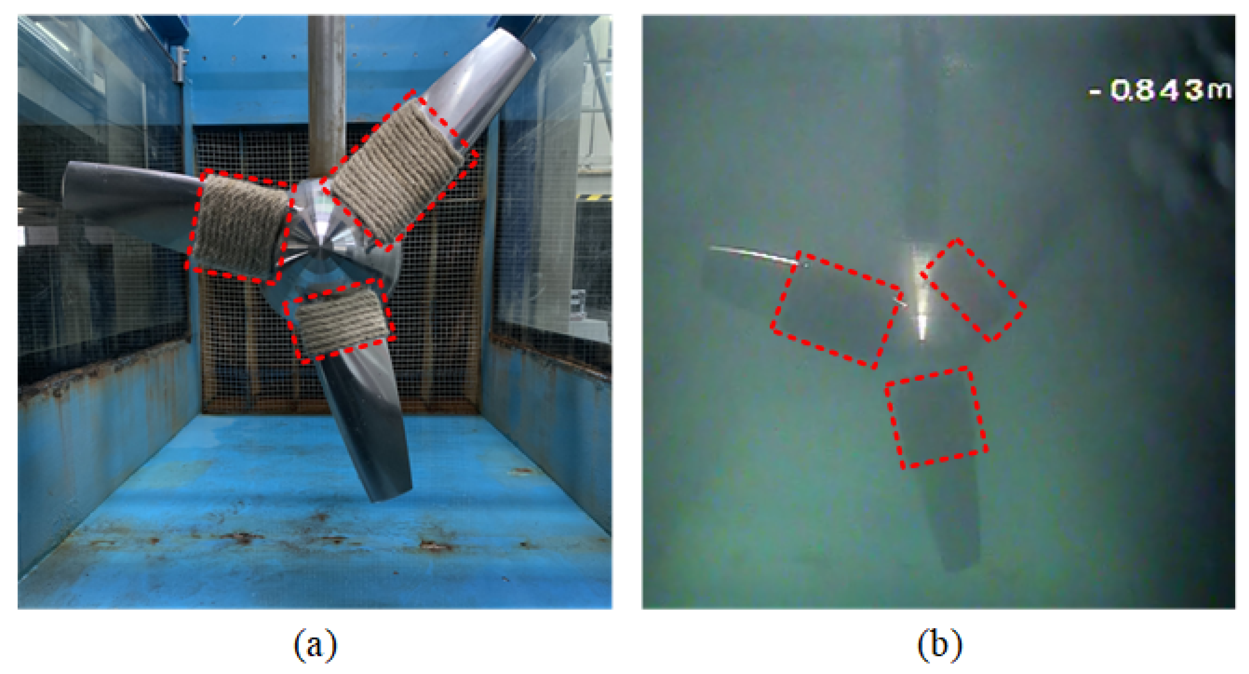
18]. The rope is used to wrap around the TST rotor to simulate the biofouling, as shown in
Figure 2. Different degrees of attachment are simulated by employing dry ropes of varying weights and different wrapping methods. Specifically, the degree of attachment is distinguished by the dry rope weight (20 g, 40 g, and 60 g), area, and position. The total number of winding turns is 13, of which there are 3 different configurations for 40 g, namely 13, 3 (near the tip)-10 (near the hub), 6 (near the tip)-7 (near the hub). The detailed attachment degrees are shown in
Table 1. The data collection experiment is carried out in two working environments of clean and turbid water. Image data collection is carried out at different shooting angles to simulate the real underwater monitoring situation. The collected data are divided into 11 categories according to the attachment degrees. The training set and test set contain
images for each category, totaling
images.
4.1.2. Network Implementation Details
The method implementation process and network have been stated in
Section 3. All the algorithms are designed by Python
. The classification network is built with open source deep learning framework TensorFlow [
45]. The details of the network parameters involved are listed in
Table 2.
4.1.3. Experiment Results
We apply the proposed MobileNet-IRNLGD rotor attachment detection network to the TST dataset to validate the effectiveness. First, we evaluate the performance of MobileNet in first-level detection.
Table 3 shows the average results of classification networks under ten repeated experiments. The dataset comes from the data collection experiment mentioned above. It can be seen that MobileNet achieves the best performance in terms of reducing the number of trainable parameters. In the case of costing
parameters of ResNet50, the accuracy of MobileNet is
higher. The two-layer CNN and VGG-16 fail to extract attachment features well due to insufficient network layers, so the recognition accuracy is unsatisfying. Moreover, because of the standard convolution, the number of parameters is dozens or even hundreds of times that of MobileNet, even if the depth is not as deep as the same. The results of two different ResNets show that the accuracy of the network does not increase significantly with the depth of the network; it can be analyzed that the TST images are captured underwater, and the contrast decreases compared with the onshore image due to the medium absorption and attenuation of light propagation. As the image intensity decreases, the features will be lost in the deep network, so the accuracy does not improve much with the increase in the network depth.
Next, we assess the performance of IRNLGD. To verify the effectiveness of the proposed algorithm in a complex underwater environment, the operating environment of the TST is divided into clean/turbid water. Each environment is further characterized by strong/weak illumination. The data under strong illumination come from Ref. [
17], and the data under weak illumination come from the data collection experiment mentioned above. Four representative edge detection algorithms are selected, including Canny, SE, HED, and PiDiNet. The mean squared error (MSE) and average gradient (AG) are employed to evaluate the performance of each method. MSE is used to evaluate the similarity of the edge detection results to the original images, while AG is used to measure the rate of gray change in the results, which reflects the clarity and the expression of detail. The quantitative evaluation results are presented in
Table 4. IRNLGD achieves the best results in both MSE and AG, indicating that the edges detected by the proposed method are closest to the original image and possess the richest details. Canny and PiDiNet are ranked second and third, respectively. The outcome is consistent with the characteristics observed in qualitative comparisons.
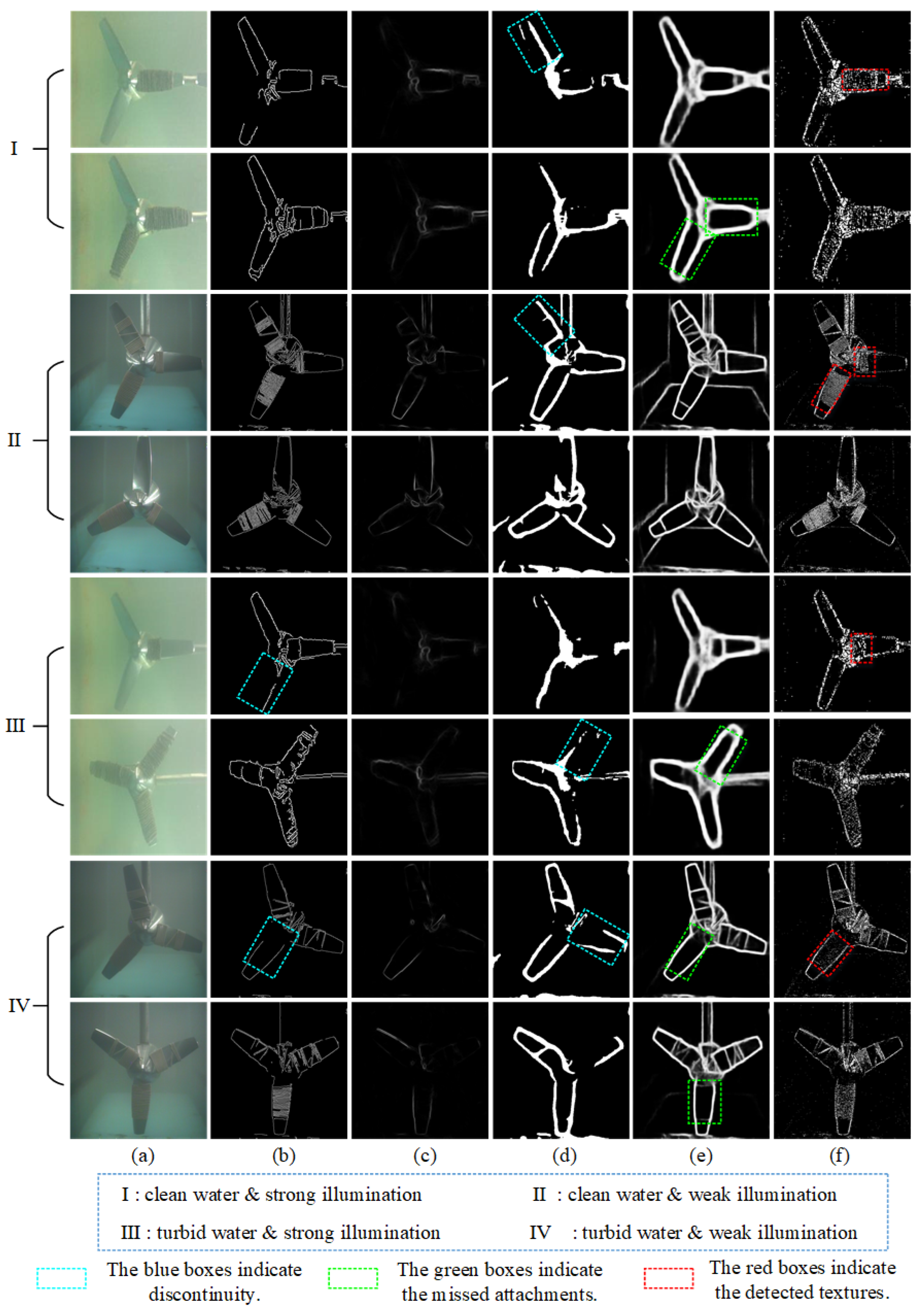
Figure 3 shows some results on the TST dataset, with two samples for each environment. The experimental results indicate that SE hardly detects meaningful edges. The results of HED and parts of Canny are discontinuous, failing to detect closed edges, as shown in the blue boxes in
Figure 3. While PiDiNet achieves the most outstanding performance among the comparative methods, its output cannot distinguish between attachments and blades. This leads to a crucial problem: when the blades are completely covered by attachments, the results from PiDiNet fail to provide meaningful information, as indicated in the green boxes in
Figure 3. Only the proposed IRNLGD can detect complete blade contours and the texture of attachments, which can achieve attachment localization (the red boxes in
Figure 3). What is more, a detailed comparison is conducted to demonstrate the advantages of the proposed method in TST attachment fault detection. The performance evaluation criteria are: (1) the ability to separate the foreground and background; (2) the ability to detect the edge of the TST rotor; and (3) the ability to distinguish between the blades and attachment.
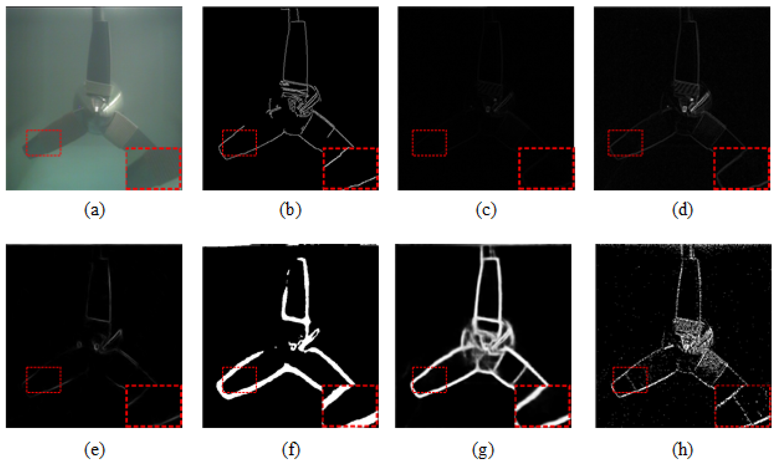
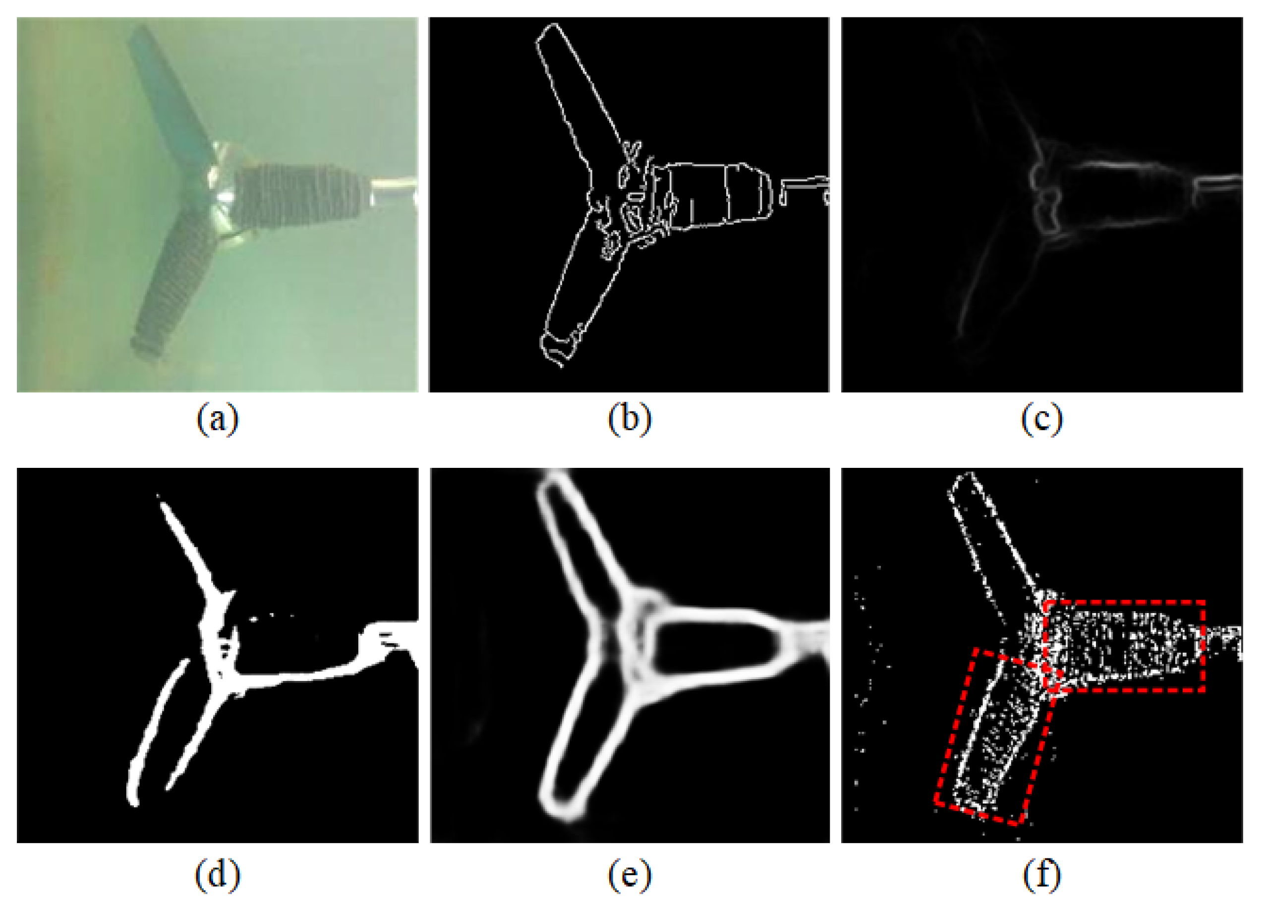
Figure 4 shows the edge detection results of the TST image under clean water and strong illumination. Canny is capable of capturing the complete edge of the TST rotor and can partially differentiate the attachment from the blades. However, the distinction may not be very clear. SE and HED fail to obtain the complete edge of the rotor. PiDiNet captures complete edges but fails to differentiate between the blades and attachment, which may affect the subsequent maintenance process. The proposed algorithm not only captures clear and complete edges of the TST rotor but also highlights the distinction between healthy blades and the attachment.
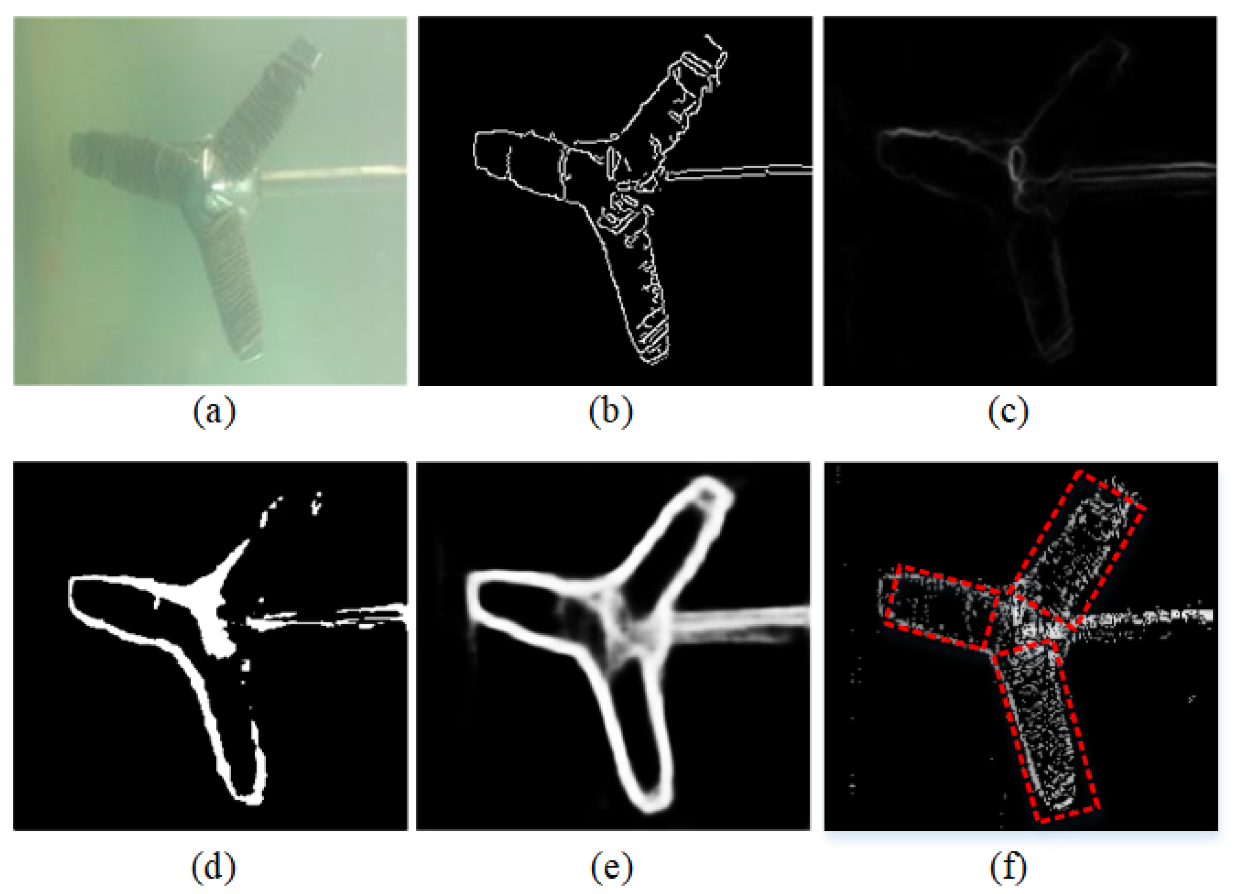
Figure 5 shows the edge detection results of the TST image under turbid water and strong illumination. Similar to
Figure 4, Canny can extract rotor edges but cannot indicate the location of the attachment. SE is almost completely ineffective, and HED detects incomplete edges. PiDiNet can detect complete edges, but they tend to be thick with insufficient refinement. It also ignores the localization of the attachment. IRNLGD is capable of both extracting complete edges and indicating attachment areas.
Figure 6 shows the edge detection results of the TST image under clean water and weak illumination. We use several boxes to highlight the details. Except for SE, most of the algorithms can detect clear edges but some differences exist: Canny and IRNLGD can extract fine edges and differentiate between clean blades and biofouling regions, while the other two can only identify the outline. HED can only detect partial edges and tends to lose edges in details, such as the attachments at the blade tip (left red box in
Figure 6d); the detected edges are incomplete, as shown in the dark side of the blade (right green box in
Figure 6d). PiDiNet can extract precise rotor edges but fails to distinguish between the blades and attachment. What is more, it also displays some edges of background, which are useless for fault diagnosis. In the comparison of Canny and IRNLGD, the attachment area detected by Canny shows partial loss (left red box in
Figure 6b), but IRNLGD can fully display the texture of the attachment (left red box in
Figure 6f). Both of them have achieved better results in edge refinement than other methods. Canny performs well in refinement due to non-maximum suppression. However, it is important to note that Canny’s high performance relies on manually selected thresholds, while the proposed IRNLGD is adaptive.
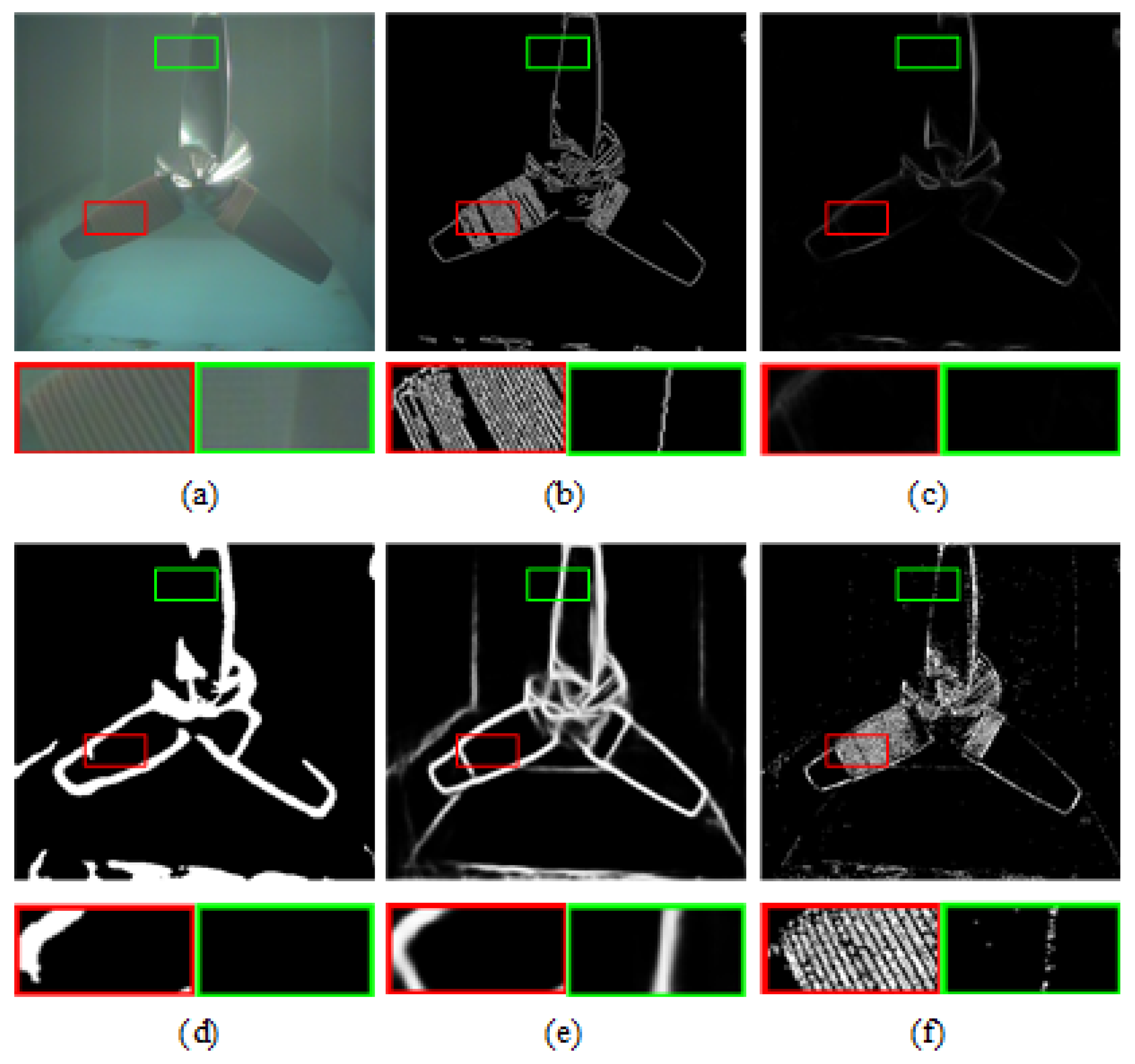
Figure 7 shows the edge detection results of the TST image under turbid water and weak illumination. SE fails to detect a meaningful edge. HED produces incomplete contours (right green box in
Figure 7d) and fails to detect the boundary between the attachment and blade near the tip (left red box in
Figure 7d). PiDiNet offers advantages in edge extraction, but it cannot indicate the attachment areas. Canny and IRNLGD perform well in distinguishing between the blade and the attachment, but Canny tends to lose details in densely textured areas (right green box in
Figure 7b). In contrast, IRNLGD not only detects complete edges but also clearly distinguishes the attachment area from the blades.
4.2. Experiment on BSDS500 Dataset
Due to the lack of a publicly available edge detection dataset designed for underwater images, the BSDS500 dataset is used to evaluate the quality of the proposed edge detection algorithm. The dataset is universally adopted for natural edge detection evaluation, consisting of 500 natural images and real human annotations. Each image is segmented by five different experts independently. The five segmentation results are combined with equal weights for objective ground truth. Color channel attenuation and blurring operations are performed on the dataset to simulate the characteristics of an underwater environment.
We employ three quantitative metrics commonly used in edge detection evaluation: the optimal dataset scale (ODS), optimal image scale (OIS), and average precision (AP).
Table 5 compares the different edge detection algorithms on BSDS500. The proposed algorithm does not obtain satisfactory results in quantitative evaluation, primarily because IRNLGD can detect fine edges, while human ground truth focuses more on contours and ignores details. This difference causes the detected detailed textures to be penalized in the evaluation. The distinctive feature can be highlighted in visual comparisons.
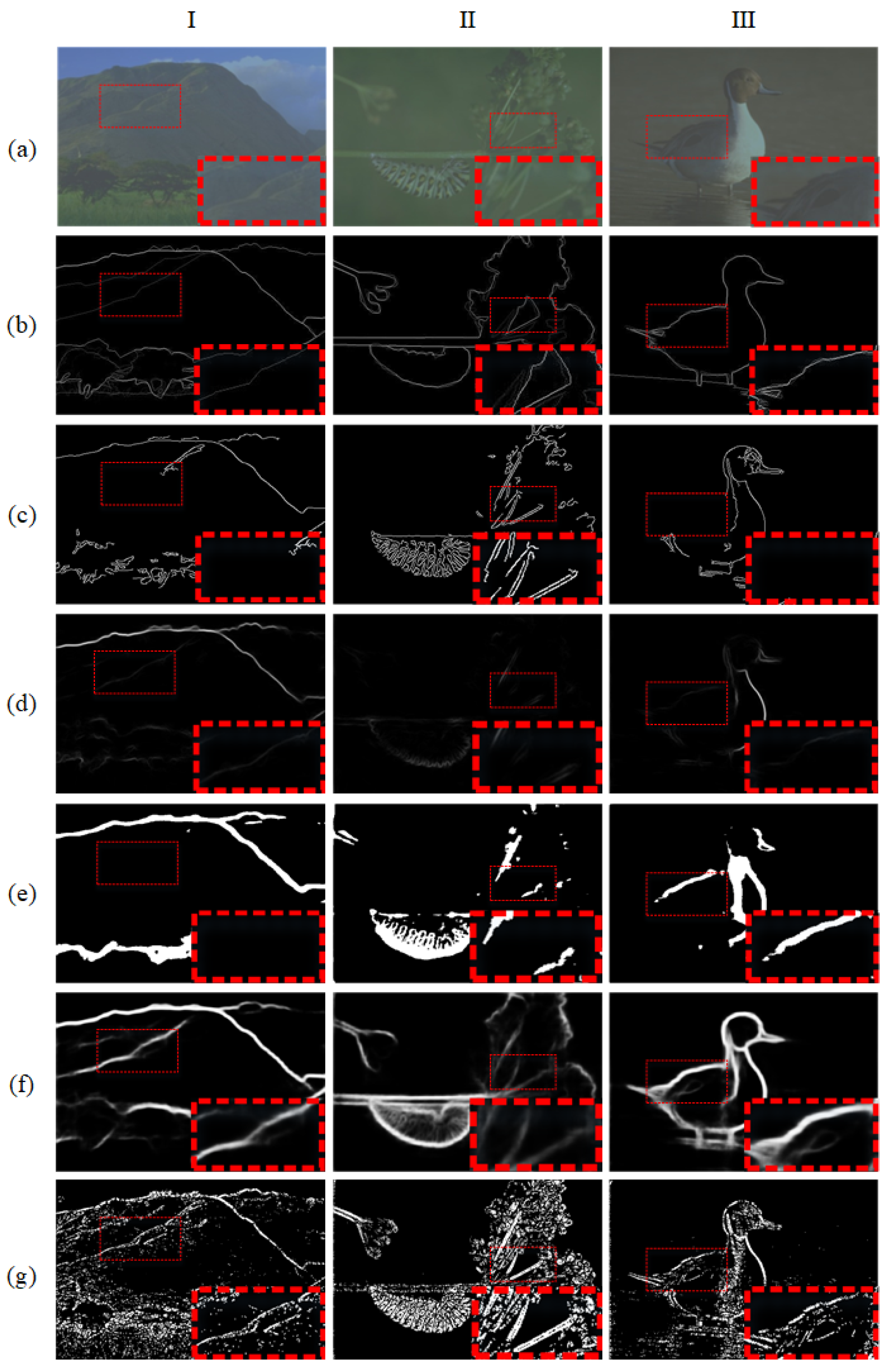
Figure 8 compares the results of IRNLGD with those of other methods. Due to the simulated underwater operation, the images are degraded and feature extraction is compromised, leading to various degrees of failure for the algorithms: SE fails to detect meaningful edges; HED produces a few non-closed contours, losing the most meaningful information, as shown in
Figure 8d,e. Canny and PiDiNet achieve better performance among the compared methods but still exhibit incomplete edges. There are discontinuities in low-contrast regions, which is evident in the results of Canny (
Figure 8c). The dependence of deep learning on data can result in decreased performance when dealing with new types of samples. For example, in
Figure 8f, PiDiNet fails to detect edges or produces weak responses in some dim areas. In contrast, IRNLGD can detect complete edges and capture details not marked in human ground truth, such as the bird wing in sample III in
Figure 8g. The proposed method may have weaker noise suppression capabilities but successfully detects complete edges and fine textures.
4.3. Experiment on UIEB Dataset
Experiments were conducted on the UIEB dataset [
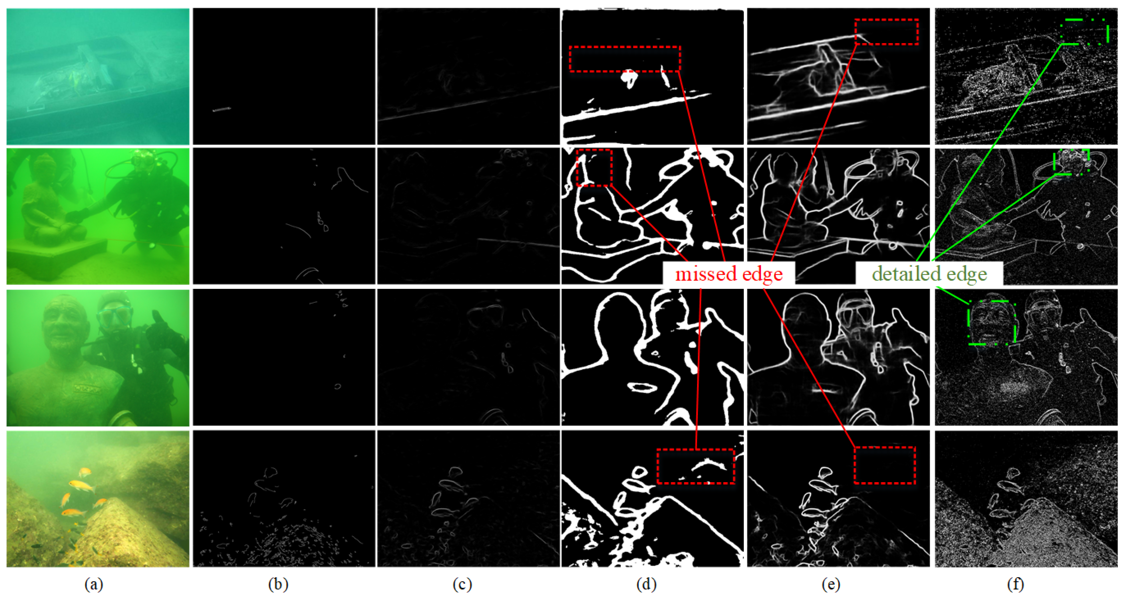
44] to demonstrate the proposed method’s effectiveness on underwater images. The dataset contains 950 original underwater images captured under various illuminations, including natural light, artificial light, or a combination of both. Due to the lack of an objective and publicly available human ground truth, only a qualitative assessment is performed here.
Figure 9 shows some detection results. Due to the degradation of underwater images, Canny and SE fail to detect meaningful edges and only prove effective in some high-contrast regions. HED produces a clear contour but can only detect partial edges in a high-turbidity environment. PiDiNet takes into account the idea of pixel differentiation and is sensitive to gradients, achieving more complete edge detection compared to HED. However, it also misses some edges, especially in low-contrast regions, as shown in red boxes in
Figure 9e. IRNLGD not only achieves complete edges but also detects fine details, even in dim parts (as shown in the green boxes in
Figure 9f). Moreover, its performance does not rely on an extensive amount of data for training.
4.4. Analysis
Based on the above experimental results, it is evident that the proposed method outperforms other techniques in the detection of fine edges in underwater images. IRNLGD obtains better results on the TST and UIEB datasets than other methods. The failure of the compared methods is due to the scattering during the propagation of light underwater, which causes image degradation. Forward scattering weakens the energy of the light, blurring the image and defocussing the contour lines; backward scattering allows light reflected by floating particles to enter the camera, resulting in an image with much noise. These factors make underwater images characterized by low contrast and attenuated intensity, leading to the failure of various edge detection algorithms that perform well in air images. The pixel values of underwater images do not vary significantly, making some gradient-based operators unable to obtain the desired results. The accuracy of supervised algorithms relies on rich training data. They fail on underwater images with low contrast due to a lack of labeled samples. However, our method considers gradients in multiple directions, allowing for the capture of richer information. Additionally, IRNLGD creatively introduces the concept of “gradient direction calibration”, enabling gradient directions to directly participate in edge determination; it contributes to IRNLGD’s ability to better capture changes in pixel intensity with limited information, thus facilitating edge detection in degraded images such as those with low light or turbidity.
In the quantitative assessment, the results of IRNLGD are undesirable. The reason is that BSDS500 is annotated for image segmentation and contour detection, and some detailed edges detected by the proposed method are penalized. However, the new edges and textures can also provide valuable information in some cases. The quantitative evaluation results of supervised algorithms are generally better due to the advantage of deep learning-based methods with good feature extraction. They can extract deep feature representations from a large number of training images. A similar feature extraction process does not exist in unsupervised methods. However, our method can still obtain satisfactory results and has no requirement for paired data for training. Therefore, the proposed IRNLGD is competent for edge detection tasks.
While the proposed method has some limitations compared with other methods, these can also be turned into advantages in certain situations. It is undeniable that, in terms of semantic understanding, IRNLGD falls short compared to deep learning-based approaches. However, the performance of deep learning relies on a large amount of labeled data, which is not aligned with the research purposes. The advantage of IRNLGD lies precisely in its ability to perform comprehensive and detailed edge detection without the need of training. Additionally, the proposed IRNLGD exhibits some noise in certain samples; this is acceptable. IRNLGD is designed for fault diagnosis in underwater equipment such as a TST, and this characteristic helps to distinguish between attachments and equipment bodies in the outcome: submerged devices often use smooth materials and anti-fouling coatings to delay biofouling, while the biofouling has a rough surface [
46,
47]. Experimental results on the TST dataset demonstrate that IRNLGD can fully display the texture of attachments, thereby indicating attachment areas; something that other methods cannot achieve. Therefore, a small amount of noise does not diminish the contribution of the proposed method to the research purposes.
In summary, the proposed method can detect fine edges better, without training or manually selected thresholds, and is more robust than other methods.
5. Conclusions
In this paper, a novel edge detection method IRNLGD based on multi-direction gradient is proposed. IRNLGD enhances the edge determination process by calibrating the gradient directions, allowing a more comprehensive inclusion of gradient from multiple directions. Experiments on a TST dataset, BSDS500, and UIEB demonstrate as follows: (1) IRNLGD can effectively detect edges in low-quality images; and (2) IRNLGD can detect a greater amount of fine texture information. In addition, we explore a two-level TST rotor attachment detection method, MobileNet-IRNLGD. IRNLGD is added as a branch to the classification network MobileNet, which provides fault location while the MobileNet provides attachment degree. The advantages of this method are: (1) It requires less computational resources, reducing hardware demands. (2) It combines supervised algorithms with non-data-driven methods to achieve complementarity, reducing the need for extensive training data. The proposed MobileNet-IRNLGD can provide preliminary fault diagnosis in the first stage, enabling technical staff to take appropriate measures based on the fault severity. During underwater cleaning operations, the precise fault localization in the second stage can provide necessary reference and guidance for operators. Since the proposed edge detection method, IRNLGD, is a non-data-driven algorithm, it can meet the monitoring needs of various types of submerged turbines and other underwater devices. This can be extrapolated from experiments conducted on the UIEB dataset, as our method can also achieve detailed edges and texture detection in degraded underwater images. Overall, the proposed IRNLGD has demonstrated its effectiveness in edge detection, and the MobileNet-IRNLGD has also shown promising results and potential.
IRNLGD can effectively extract edge information from TST images without requiring paired data for training. However, it faces challenges when dealing with images affected by motion blur. In the future, the research will focus on exploring solutions for the motion-blurred images.


