Investigating Load Calculation for Broken Ice and Cylindrical Structures Using the Discrete Element Method

Abstract

Ice loads are critical forces that impact the structural integrity of offshore equipment in high-latitude sea areas and play a pivotal role in the design of structures in ice-prone regions. The primary objective of this study is to investigate both experimental and numerical approaches to analyze ice loads on marine structures, elucidate their characteristics and patterns, and offer technical support for the design of structures in ice-prone areas. To achieve this goal, an ice model was built using polypropylene material, and experiments were conducted in a wave flume at room temperature to measure the ice resistance on cylindrical structures. Structural loads were assessed at various ice velocities while maintaining a fixed ice concentration. Furthermore, a high-performance discrete element technology was employed to develop a numerical simulation method for calculating ice resistance on cylindrical structures. Sensitivity analysis was conducted to evaluate the influence of discrete element density on the resistance outcomes. The predicted structural resistance for ice velocities corresponding to the experimental conditions was compared with the results obtained from the model experiment. The research findings indicate that the primary cause of ice resistance is the interaction between the structure and fragmented ice, which leads to collisions, friction, rotation, and local ice accumulation. To quantify the resistance, ice resistance coefficients were defined using an average resistance formula, representing different statistical values. These coefficients were found to remain relatively constant at varying sailing speeds. The results obtained through the discrete element method for ice resistance demonstrated a remarkable agreement with the experimental findings, both in terms of observed phenomena and numerical values. This agreement serves as evidence substantiating the effectiveness of the numerical approach. These methods offer efficient and accurate load prediction solutions for the design of structures in cold regions.

1. Introduction

Ice loads are crucial control loads that impose safety limitations on offshore equipment structures in high-latitude marine regions. They constitute vital input parameters for designing marine structures with ice-strengthened features, such as lighthouses, conductor support platforms, and wind turbine foundations, which can be approximated as vertical cylindrical structures. The interaction between ice and cylindrical structures results in substantial ice loads and dynamic responses in the structures. Icebreakers are commonly employed to break level ice into broken pieces as a risk mitigation measure. Broken ice exerts notable effects on structures, such as collision, accumulation, rotation, and friction. Consequently, investigating the interaction loads between broken ice and cylindrical structures carries considerable practical importance.

Recently, there has been global attention toward the prediction and analysis techniques of ice loads. Timco [1,2,3] summarized experimental data related to the impact of floating ice on offshore structures. Experimental data regarding the impact of floating ice on offshore structures were summarized. By taking into account the kinetic energy of floating ice, empirical formulas were derived based on ice mass and velocity to determine the load on structures caused by broken ice. The discrete element method (DEM), based on the discontinuous medium approach, has been utilized to capture the nonuniform, discontinuous, and large deformation characteristics of sea ice. Significant progress has been made in this method in recent years, owing to advancements in computer hardware. Ji et al. [4,5,6] developed a FEM–DEM coupled method that allows for the simulation of the dynamic response of the interaction between structures and ice layers. They employed a GPU parallel algorithm to enhance computational efficiency and developed a rapid generation model for fragmented ice. By utilizing a fast search algorithm among polyhedra and a cohesive-fracture model, they improved the accuracy of analyzing structural ice loads and established a convenient computational tool. Jou et al. [7] modeled sea ice using the local cohesive discrete element method. They investigated the collision between level ice and inclined icebreaking cones at various angles and compared the results with other DEM simulations.

The cohesive zone model (CZM) has been used to simulate the interaction between level ice and structures [8,9,10,11,12,13]. Theoretical methods were utilized to determine the initial stiffness, reducing the dependence on grid resolution in the cohesive element approach. In a previous study, a numerical model using the FEM–SPH adaptive method was developed to investigate the interaction between conical objects, icebreakers, and level ice. By comparing the model results with experimental data, the study demonstrated the potential of this method in accurately simulating ice fragmentation resistance [14].

Research on icebreakers has made significant advancements due to the growing demand for Arctic scientific expeditions. Xue [15] provided a comprehensive summary of the latest experimental techniques in studying ice loads, particularly emphasizing their application to ships, and conducted extensive foundational studies in this area. Dynamic methods have been employed by researchers to examine the impact of factors, including ice thickness and navigation speed, on average ice loads [16,17]. Wang developed a time-domain numerical calculation method to assess the icebreaking capabilities of ships by studying continuous icebreaking loads and ship motions [18]. Furthermore, utilizing LS-DYNA simulations of collision-induced icebreaking contact loads, additional investigations were carried out to analyze the bending moments and structural loads on the ship’s cross-section [19].

Several researchers have investigated ice loads in broken ice environments through experimental methods. Zong et al. conducted scaled model towing experiments employing a polypropylene ice model to examine the influence of broken ice concentration, ice block shape, and size on ship resistance. Additionally, they also confirmed the viability of employing the polypropylene ice model for studying ice resistance [20,21]. Islam et al. [22,23] employed model testing methods to investigate ship motion, loads, and maneuvering performance in ice-covered waters. Furthermore, they analyzed the loads on the ice–structure interface, thus affirming the potential of discrete element methods in engineering applications.

Sea ice is composed of discrete floating blocks that exhibit substantial variations in size. Roach et al. [24] introduced a joint distribution model to characterize the thickness and block size of sea ice, and this model effectively captures the fluctuations in ice thickness, leading to enhanced simulations of ice–structure interaction loads. Li et al. employed measured data from Antarctic research vessel expeditions to derive probability distributions that yield the best fit for ice loads through statistical analysis. These probability distributions form a basis for long-term statistical analysis, thereby facilitating the investigation of ice-induced loads [25,26]. Huang [27] conducted dynamic ice load tests at varying ice velocities to examine the vibration process of ice-induced flexible structures and investigated the mechanisms behind vibration suppression. Their findings suggest that the control mechanism for steady-state vibration in ice-induced flexible column structures can be attributed to the periodic impact of ice loads. Moreover, the interaction between the structure and fragmented ice, along with the periodic destruction of the ice layer, exacerbates the influence of structural vibration.

Considering all the abovementioned studies, the analysis of ice loads on floating structures operating in icy environments highlights the superior accuracy of broken ice loads in representing the actual load characteristics, owing to their inherent stochastic nature. However, predicting these loads poses significant challenges. To gain further insights into the mechanisms of broken ice loads and explore the methods for predicting the interaction between broken ice and structures, this study specifically investigates the interaction between a cylindrical structure and broken ice. By employing model similarity criteria, experiments were conducted in a wave flume at room temperature using an ice model made of polypropylene to assess the resistance of the cylindrical structure to broken ice. The experiments measured the structural loads under different ice velocities while maintaining a fixed density of broken ice. Leveraging high-performance discrete element technology, a simulation method was developed to estimate the resistance of the cylindrical structure to broken ice, and a sensitivity analysis was conducted to examine the impact of discrete element density on the resistance results. The structural resistance corresponding to the ice velocity employed in the experiments was predicted, and the findings were compared with the model experiments.

2. Design for Broken Ice Load Testing

2.1. Experimental Configuration

As previously mentioned, broken ice loads predominantly arise from the collision forces occurring between the ice and the structure. Consequently, when conducting experimental tests on an upright cylindrical model to investigate ice loads, the emphasis lies on simulating the impact load resulting from broken ice on the structure and exploring the correlation between structural ice loads and the velocity of the floating ice. Polyethylene, possessing strength comparable to that of authentic sea ice, can be employed as the material for fabricating the ice model, which interacts with the structure. The experimental model was partitioned into multiple sizes in accordance with the structural scale.

To isolate the effects of broken ice loads on the cylindrical structure, it is essential to determine the components of fluid loads that act on the structure. Therefore, separate model experiments were conducted in ice and ice-free environments, followed by data processing to differentiate the broken ice loads.

After successfully preparing the ice model, the experimental process was divided into three main parts:

(1)

The installation of the experimental model, calibration of sensors, and debugging of the testing system;

(2)

The generation of a controlled flow to assess the fluid loads on the cylindrical structure at various flow velocities;

(3)

In the presence of ice, the ice model was propelled by the flowing water, causing it to move with the flow and come into contact with the structure.

Multiple experiments were carried out for each working condition to ensure the stability of data collection. Figure 1 illustrates the experimental system and its associated equipment, and Figure 2 presents the schematic diagram of the actual experimental setup.

2.2. Criteria for Experimental Similarity

In the present study, we focused on investigating the influence of various factors, including gravity, inertia, viscosity, elastic forces, and dynamic friction, arising from the interaction between the structure and ice. Special attention was given to ensuring the similarity of Froude numbers (Fr) and Cauchy numbers (Ca) between the model system and the prototype system. To achieve this, scale ratios were employed. Considering the dimensions of the marine riser structure, which measured 0.55 m, and considering the experimental conditions, including wave and flow flume, a scale ratio of 55 was selected for this study. Furthermore, the experimental data collected correspond to the actual operating conditions, as depicted in

Table 1. Scaled operational data for ice–structure parameters.

Parameters	Model	Real Structure	Ratio
Cylinder diameter (m)	0.01	55	$\lambda =55$
Ice velocity (m/s)	0.20	1.48	${\lambda }^{\frac{1}{2}}$
Ice thickness (m)	0.004	0.22	$\lambda$
Broken ice scale (m)	0.008	0.40	$\lambda$
Ice force (N)	/	/	${\lambda }^3$

and

Table 2. Experimental load case and scaling parameters.

No.	Load Case Name	Experimental Velocity	Actual Velocity	Ca	Fr
1	LC1	0.050 m/s	0.371 m/s	1.547 × 10−7	0.187
2	LC2	0.075 m/s	0.556 m/s	2.319 × 10−7	0.281
3	LC3	0.125 m/s	0.927 m/s	3.866 × 10−7	0.468

. This approach enhances the academic rigor of investigation by considering crucial aspects and establishing connections between the model experiments and real structure.

3. Numerical Method

3.1. DEM Theoretical Approach

a

Ice Discrete Element Model

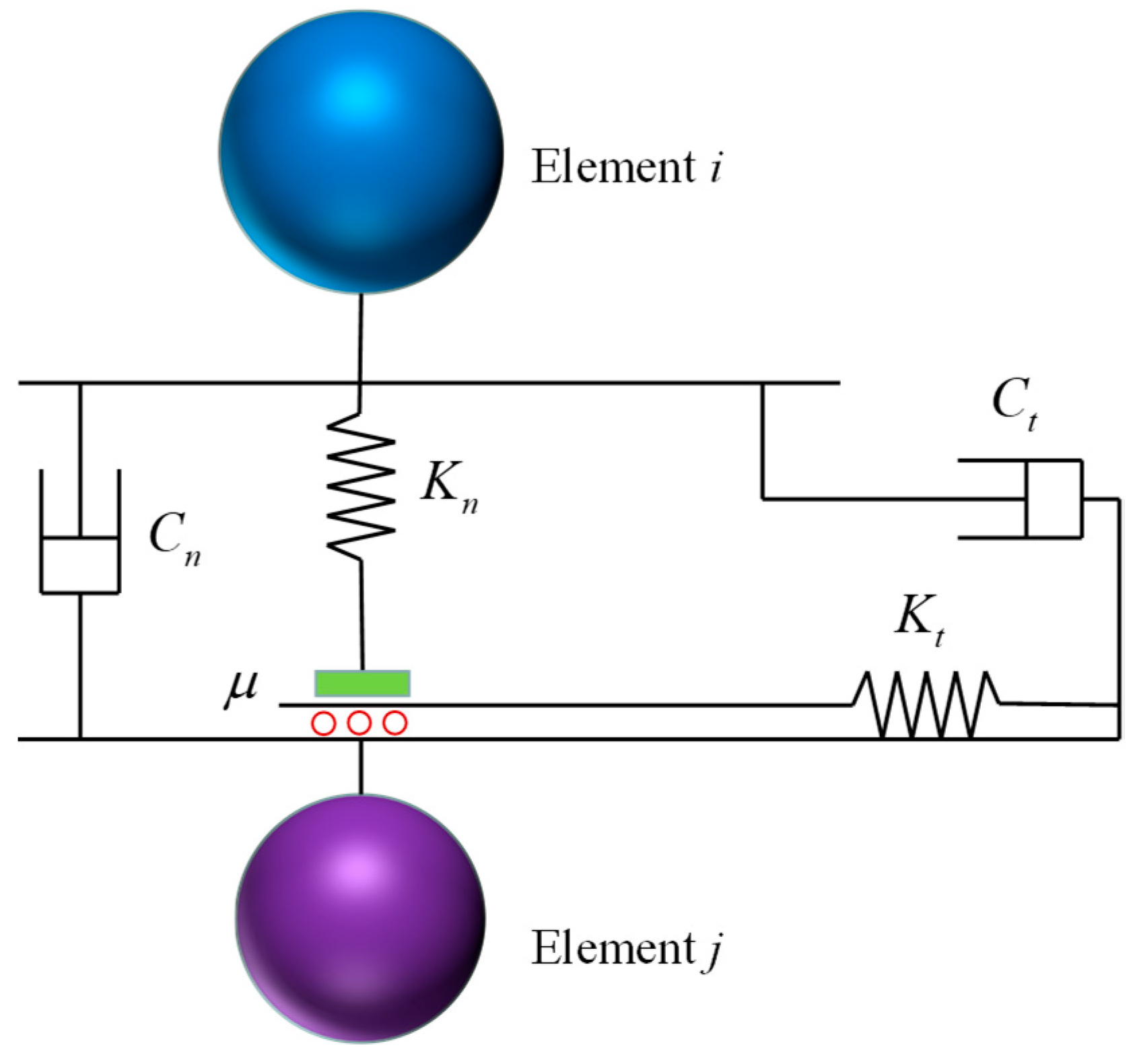
Sea ice is conceptualized as an assembly of discrete particles, wherein individual particles exhibit a relatively independent motion but engage in interactions upon contact. To simulate the collision process between particle units, a spring–damper–slider model [5] was employed, as depicted in Figure 3. This modeling approach allows for a comprehensive representation of the dynamic behavior of sea ice, capturing the effects of particle interactions and their subsequent motion.

The forces $\mathit{F}$ generated by each unit are calculated by summing the normal contact force ${\mathit{F}}_n$ and the tangential contact force ${\mathit{F}}_{\tau }$.

$$\mathit{F}={\mathit{F}}_n+{\mathit{F}}_{\tau }$$

(1)

The normal contact force $F_n$ can be expressed as the sum of the normal elastic force $F_n^e$ and the normal viscous force $F_n^v$, that is,

$$F_n=F_n^e+F_n^v$$

(2)

$$F_n^e=k_n{\delta }_n^{3/2}$$

(3)

$$F_n^v=c_n\sqrt{{\delta }_n}{\dot{\delta }}_n$$

(4)

where $k_n$ is the normal contact stiffness coefficient; ${\delta }_n$ is the normal overlap between particles; $c_n$ is the normal damping coefficient; and ${\dot{\delta }}_n$ represents the relative normal velocity.

$$k_n=\frac{4}{3}{E}^{*}\sqrt{R^{*}}$$

(5)

$$c_n={\zeta }_n\sqrt{m^{*}{k}_n}$$

(6)

$${\zeta }_n=\frac{-\ln e_0}{\sqrt{{\pi }^2+{\ln }^2{e}_0}}$$

(7)

where $E^{*}$ is the effective elastic modulus; $R^{*}$ is the effective radius; ${\zeta }_n$ is the damping coefficient; $m^{*}$ represents the effective mass; and $e_0$ is the restitution coefficient of the unit.

The tangential contact force $F_{\tau }$ can be expressed as the sum of the tangential elastic force $F_{\tau }^e$ and the tangential viscous force $F_{\tau }^v$, that is,

$$F_{\tau }=F_{\tau }^e+F_{\tau }^v$$

(8)

$$F_{\tau }^e=\mu \left|F_n^e\right|\left[1-{\left(1-\frac{{\delta }_t}{{\delta }_{\tau }^{\max }}\right)}^{1.5}\right]$$

(9)

$$F_{\tau }^v=c_{\tau }\sqrt{\frac{6\mu m^{*}\left|F_n^e\right|\sqrt{1-{\delta }_{\tau }/{\delta }_{\tau }^{\max }}}{{\delta }_{\tau }^{\max }}}{\dot{\delta }}_{\tau }$$

(10)

In these equations, $\mu$ represents the friction coefficient; ${\delta }_{\tau }$ is the tangential overlap; $\nu$ is the Poisson’s ratio; ${\dot{\delta }}_{\tau }$ is the relative tangential velocity; $c_{\tau }$ represents the tangential damping coefficient; and ${\delta }_{\tau }^{\max }$ represents the maximum tangential overlap, which can be determined using the following equation:

$${\delta }_{\tau }^{\max }=\mu \left[{\delta }_n\left(2-\nu \right)\right]/\left(2-2\nu \right)$$

(11)

$$c_{\tau }=c_n/\left(2+2\nu \right)$$

(12)

b

Coupled method of DEM and FEM

In this study, the coupled DEM–FEM algorithm proposed by Ji [28] was applied to facilitate parameter transfer between the two computational domains in the coupled DEM–FEM model established for investigating the interaction between ice and a cylindrical structure. The collision detection between fragmented ice and the cylindrical structure was simplified by considering the contact between spherical and triangular elements, with the theoretical algorithm elaborated in [29]. The conversion of particle interaction loads on shell elements to nodal loads was accomplished using the shape function method. 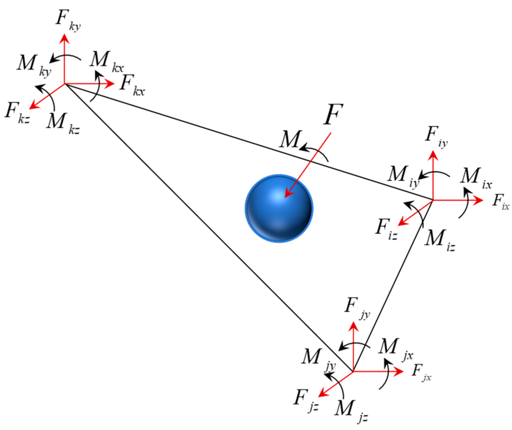Figure 4 illustrates a schematic representation of the collision contact between a single particle and a specific triangular element on the outer surface of the cylindrical structure. The calculation of the equivalent nodal forces for triangular elements is presented as follows:

$${\left\{F\right\}}_{18\times 1}={{\displaystyle {\sum }_{a=1}^p\left[T_{t,3}\right]}}_{18\times 18}^{\mathrm{T}}{\left\{N_a\right\}}_{18\times 6}^{\mathrm{T}}{\left[T_{t,3}\right]}_{6\times 6}^{\mathrm{T}}{\left\{W_a\right\}}_{6\times 1}$$

(13)

In the above equation, $N_a$ denotes the interpolation matrix for the element contacted by particle a, p represents the number of contact points exerted on the triangular element by particles, $W_a$ denotes the forces and moments exerted by particles on the triangular element, and $T$ represents the transformation matrix.

Figure 4. Contact force–moment conversion diagram of triangle element.

Figure 4. Contact force–moment conversion diagram of triangle element.

3.2. Numerical Model

a

Structure and Broken Ice Model

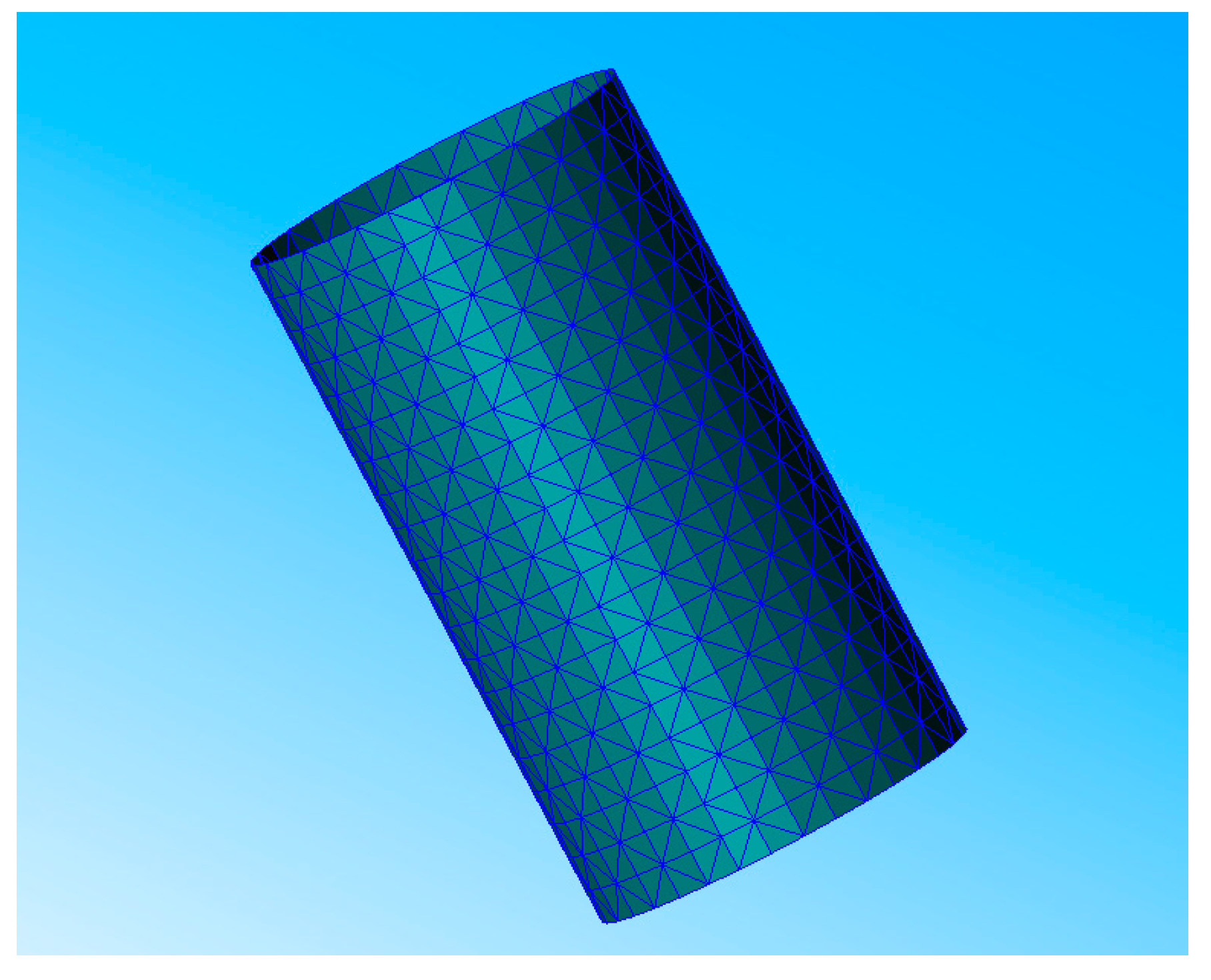
In order to compare the obtained results with experimental data, a vertical cylindrical structure with a diameter of 0.55 m was selected as the subject of analysis in this study. The outer surface of the cylindrical structure was discretized using triangular elements to comply with the internal contact algorithm utilized in this study, as depicted in Figure 5. The total element number of the cylindrical structure was 1400.

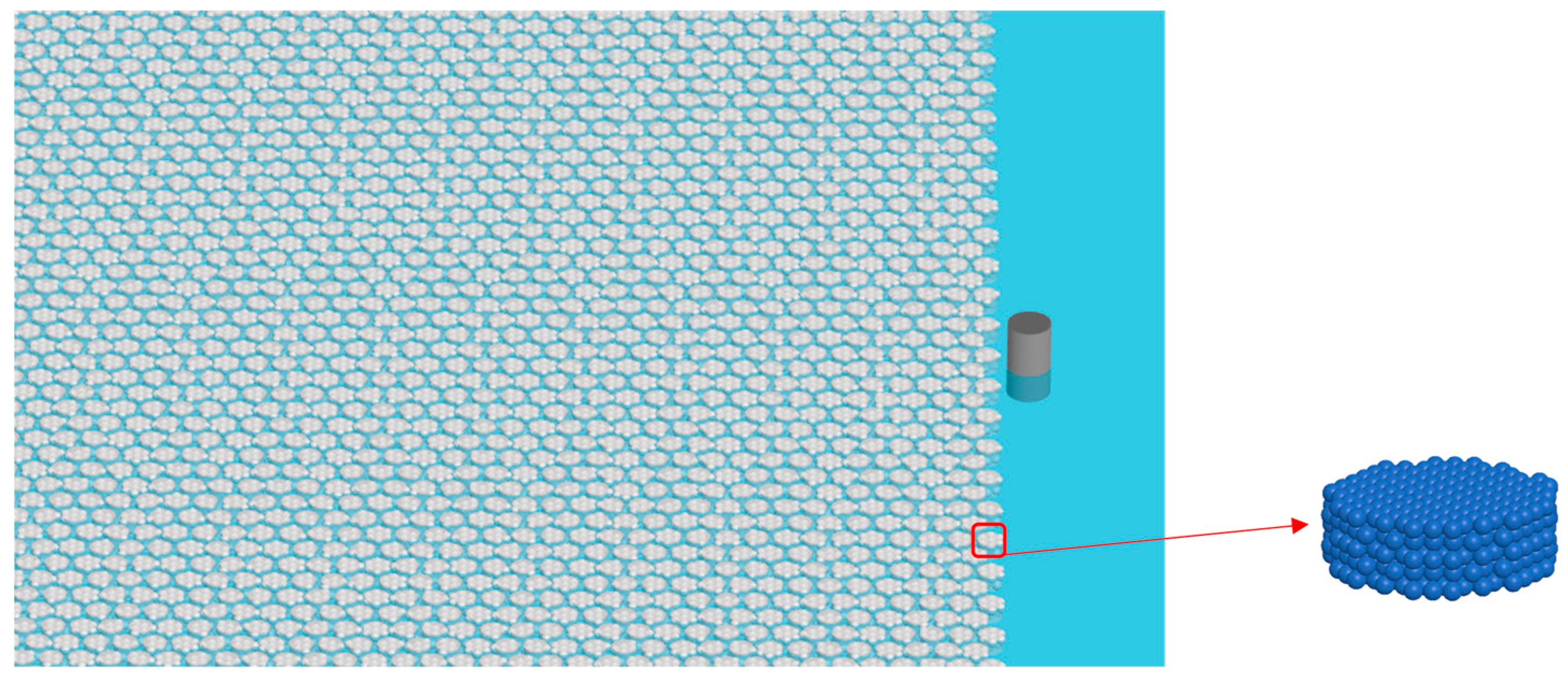
In this research, the SDEM computational program was employed to simulate the load interaction between ice and the structure. We disregarded the influence of waves and exclusively focused on the interaction between broken ice and the structure under steady flow velocity conditions. In order to mitigate the influence of boundary effects on the numerical simulation results, a computational domain measuring 100 m in length and 40 m in width was established. The density of the broken ice loads was set to 70%. Figure 6 depicts the discrete element coupled model that elucidates the interaction between the ice and the cylindrical structure. In order to ensure the reliability of the computational results, a minimum increment step of 10⁻⁶ s was used.

b

Discrete Density Comparison

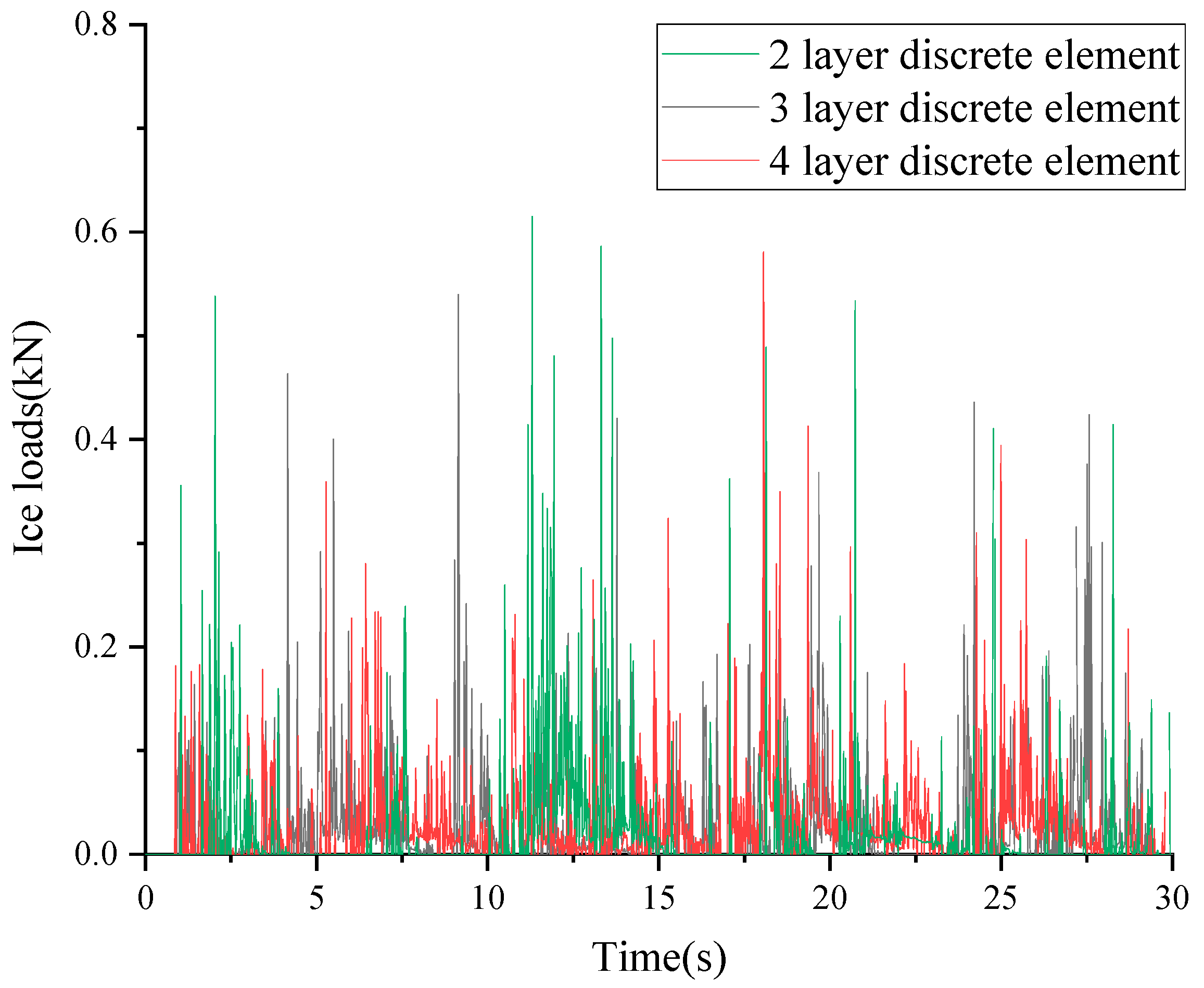
In discrete element algorithms, the term “discrete density” refers to the quantity or distribution density of particles within a specified region. Variations in discrete densities can significantly influence computational results and computation time. In order to assess the impact of discrete element density distribution on computational outcomes, a comparative analysis was conducted involving various particle distribution configurations, namely two layers, three layers, and four layers, with respect to a standardized ice thickness of 0.2 m. The number of discrete elements was 169,282, 533,264, and 1,220,996, respectively. The time-domain curves of the ice load are shown in Figure 7.

To calculate the statistical values of random loads, three distinct statistical parameters were considered: the mean ice load, the significant ice load, and the maximum ice load. The mean ice load signifies the average value derived from all ice force measurements, providing an overall representation of the data. In contrast, the significant ice load specifically pertains to the ice force magnitude throughout the entire observation period. The maximum ice load refers to the highest recorded ice force value observed over the complete duration of the study.

The statistical method employed for significant wave height was utilized and adapted for the significant ice load. The step-by-step procedure was as follows:

(1)

Time-history data pertaining to ice forces, obtained through either measurements or calculations, were acquired;

(2)

The peak ice forces, corresponding to the maximum values within the dataset, were determined;

(3)

The filtered ice forces were arranged in descending order and organized from the highest value to the lowest;

(4)

The significant ice force was calculated by averaging the top one-third of the sorted ice forces.

The resultant ice force values for each computational scenario are succinctly presented in

Table 3. Discrete density comparison parameters.

No.	Discrete Element Layers	Significant Ice Force	Simulation Time	Computation Time
1	2	0.364	30 s	13 h
2	3	0.355	30 s	60 h
3	4	0.369	30 s	144 h

.

Based on the findings presented in Table 3, it is evident that the statistically obtained ice load values exhibit minimal discrepancies across the three density distributions. However, there is a notable contrast in computational time for simulations of the same duration, and the computational times for the three different discretization densities are 13 h, 60 h, and 144 h, respectively.

Nonetheless, this outcome is intricately linked to the scale of the analyzed sea ice. Enhancing the discrete density has the potential to yield more precise simulation outcomes. By augmenting the number or density of particles, the discrete element algorithm can aptly capture the interactions and behavior among particles within the system. Consequently, conducting a sensitivity analysis of the grid scale becomes imperative within the realm of engineering research.

In order to enhance computational accuracy and optimize computational resources, a two-layer discrete element approach was effectively employed in this specific case to simulate the resistance of fragmented ice for an ice thickness of 0.20 m.

4. Results and Discussion

4.1. The Results of the Ice–Structure Test

a

Experimental phenomena

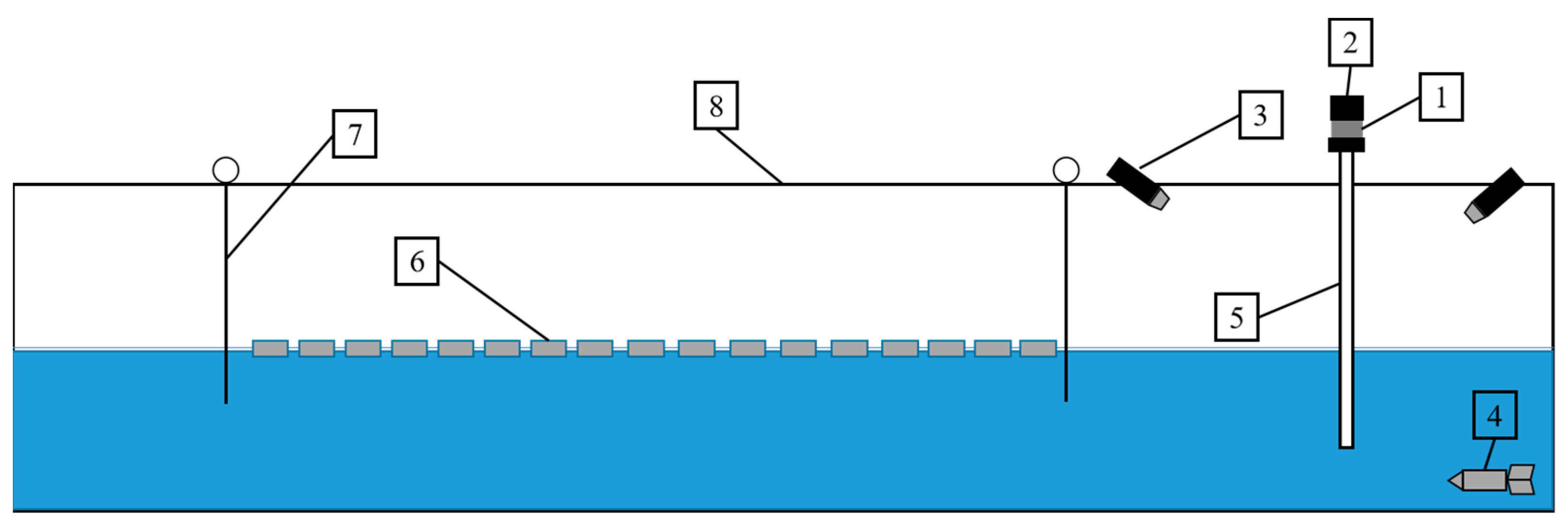
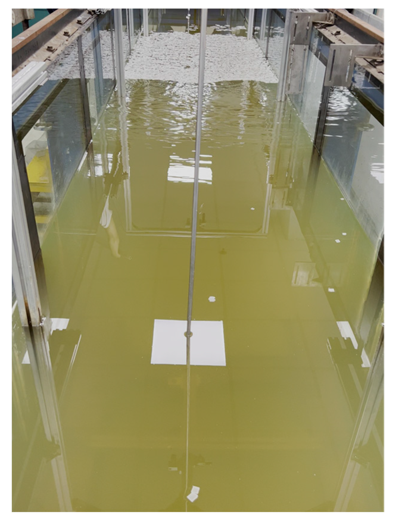
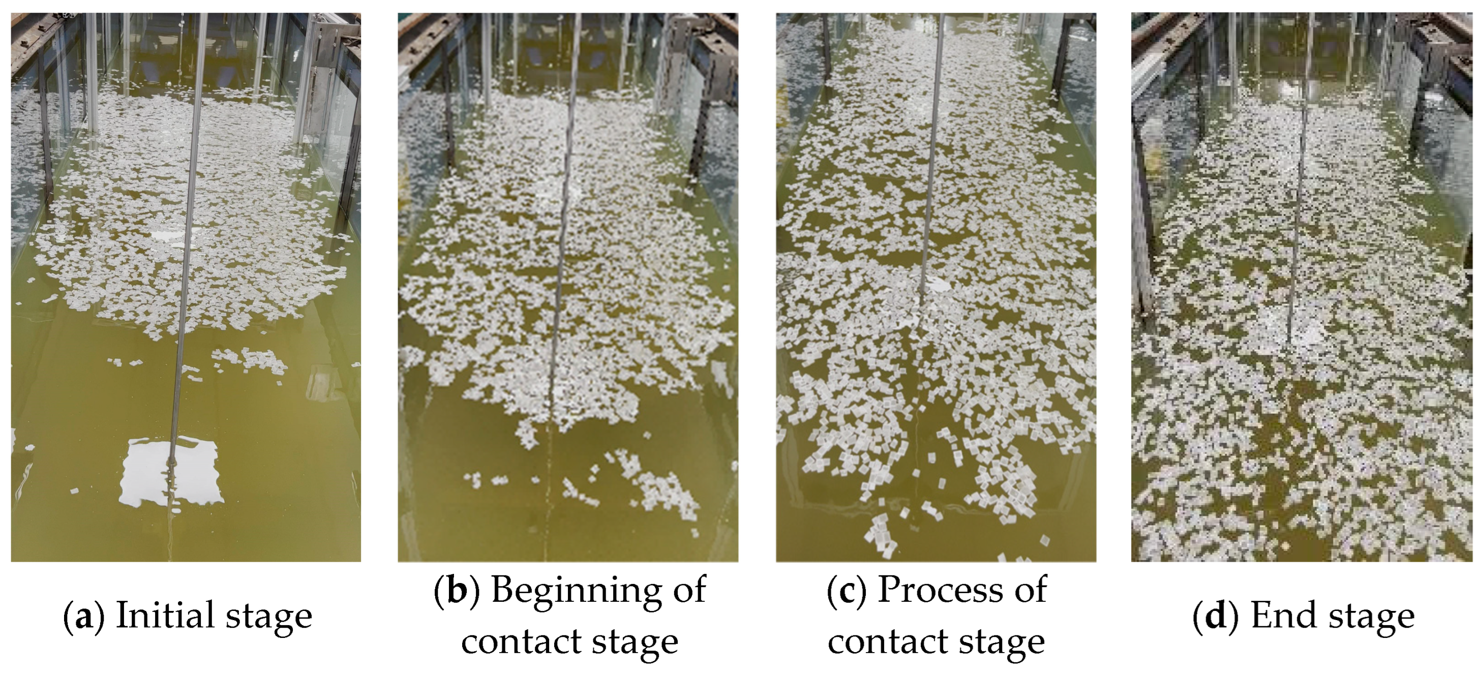
The experimental phase of the ice–cylindrical structure load is illustrated in Figure 8. Initially, in the experiment, broken ice approached the cylindrical structure at a constant velocity influenced by the flow load. Throughout the experiment, the broken ice underwent rotation or experienced friction upon colliding with the structure, leading to a subsequent alteration in its original direction of movement and dispersion toward the sides or rearward. This interaction resulted in the accumulation and clustering of broken ice. The ice–structure interaction had a brief duration, displaying periodic impact characteristics. Downstream, particularly at the rear of the cylindrical structure, a relatively unobstructed water pathway developed, as depicted in Figure 8c, exhibiting a notable contrast to the initial configuration. The interaction between the ice model and the structure exhibited evident random phenomena, consistent with relevant studies in the literature [20].

At higher ice velocities, the frequency of collisions between the broken ice and the cylinder intensified, causing the broken ice to swiftly pass the cylindrical structure. Consequently, some of the broken ice accumulated behind the cylinder, as illustrated in Figure 8d.

b

Ice load characteristic analysis

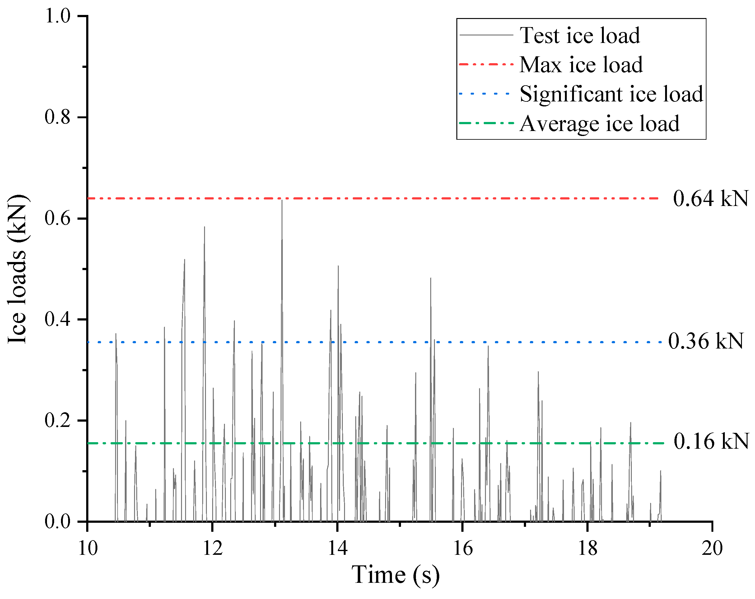
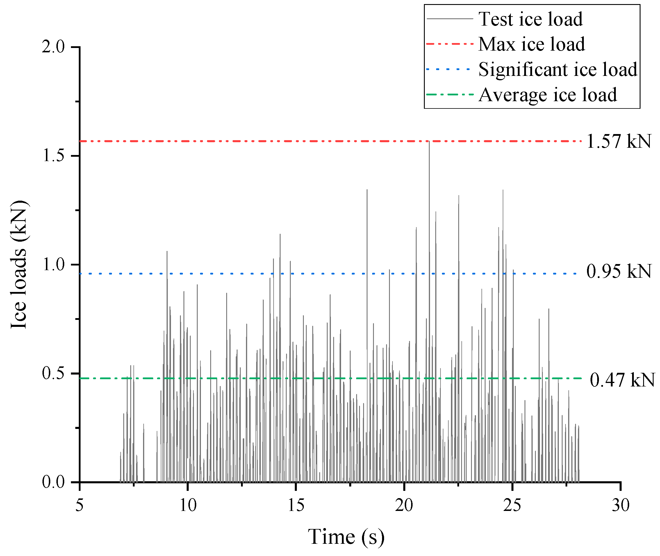
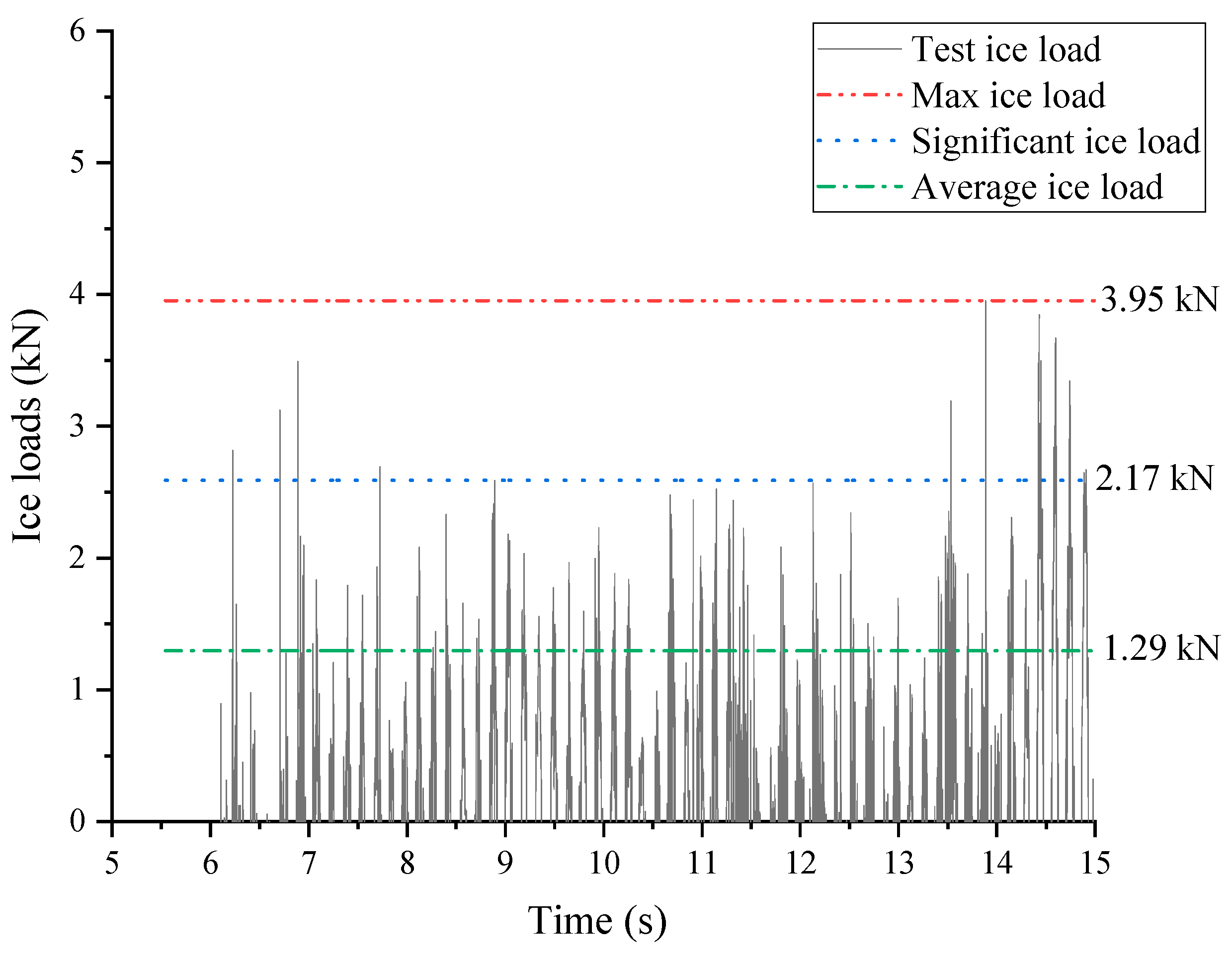
Figure 9, Figure 10 and Figure 11 illustrate the time-domain curves of the ice load determined based on scaled experimental data under three distinct velocities: 0.05 m/s, 0.075 m/s, and 0.125 m/s. Taken together, these experimental findings reveal the prominent characteristics of random loading in the ice load behavior. In the case of cylindrical structures, the experimental results predominantly indicate collisions. Conversely, for upright structures lacking slopes, the occurrence of load accumulation or climbing phenomena was relatively infrequent. This can be attributed to the dispersion of broken ice around cylindrical structures under the influence of flow velocity, inhibiting the manifestation of accumulation. Notably, the ice load exhibited a distinct triangular loading–unloading pattern.

The distribution of load curves at varying ice velocities revealed that higher velocities led to increased load frequencies and a more densely distributed set of time-history curves, aligning with experimental observations. Despite the significant randomness of ice loads and the probabilistic nature of collisions between broken ice and the structure, the overall amplitude distribution of the loads remained consistent. The time history of ice loads demonstrated distinct pulse characteristics and periodicity, consistent with the research findings of numerous scholars.

Table 4. Statistical values of experimental ice load.

Load Case	Test Velocity	Actual Velocity	Average Ice Load		Significant Ice Load		Max Ice Load
			Statistical Result (kN)	Ice force Coefficient	Statistical Result (kN)	Ice Force Coefficient	Statistical Result (kN)	Ice force Coefficient
LC1	0.05 m/s	0.371 m/s	0.16	1.14	0.36	2.56	0.64	4.55
LC2	0.075 m/s	0.556 m/s	0.47	1.49	0.95	3.00	1.57	4.96
LC3	0.125 m/s	0.927 m/s	1.29	1.47	2.17	2.47	3.95	4.49

presents the statistical findings of ice loads under various experimental conditions. The mean, significant, and maximum values of the overall ice loads were positively correlated with the experimental ice velocity. This is a consequence of the increased kinetic energy of broken ice at higher velocities, resulting in a stronger impact on the structure. Specifically, in LC2, where the ice velocity was 1.5 times that of LC1, the corresponding statistical load values were 2.94 times, 2.64 times, and 2.45 times greater than those in LC1. Similarly, in LC3, with an ice velocity 2.5 times higher than LC1, the corresponding statistical load values were 8.06 times, 6.02 times, and 6.17 times greater than those in LC1. This comparison demonstrates the nonlinear growth of loads, tending to follow a square relationship with velocity. This relationship can be attributed to the power-law distribution of characteristic ice sizes, with the power exponent ranging between 1 and 2 [30]. The fractal distribution of broken ice in space is a widely recognized characteristic.

To delve deeper into the characteristics of broken ice load amplitudes, a provisional relationship coefficient of 2 was assumed. The dimensionless coefficients of broken ice loads for different conditions were then calculated using Equation (13) to explore their inherent attributes. A comparison of the ice force coefficients revealed that while there were slight differences in the ice force coefficients for the same statistical sample under different ice velocities, the overall distribution range remained relatively constant. The ice force coefficient for average ice force was approximately 1.37, whereas the coefficient for significant ice force was approximately 2.68, and the coefficient for maximum ice force was around 4.67.

This highlights the feasibility of conveniently defining the coefficient of broken ice loads in simulations, enabling the rapid prediction of broken ice loads on multiscale ocean structures and holding significant engineering implications.

$$C_{ice}=\frac{F_{ice}}{\frac{1}{2}{\rho }_{ice}{v_{ice}}^{2}S}$$

(14)

In this equation, $C_{ice}$ indicates the ice load coefficient, $F_{ice}$ is the total ice load, ${\nu }_{ice}$ is the ice velocity, ${\rho }_{ice}$ is the ice density, and $S$ represents the area of interaction.

To verify the experimental results with actual sea ice, we referred to the literature [31] and relevant research findings to conduct experiments on cylindrical and flat ice. By calculating the ice force coefficient, it was found that, at an ice velocity of 0.125 m/s, the overall statistical ice force coefficient was 2.95. Compared to the LC3 condition in this study, which had a meaningful ice force coefficient of 2.19, the difference was 25%. Considering the fact that we used a 70% density of fragmented ice, it can be seen that the overall ice load is relatively close, which demonstrates the validity of the experimental results in this study.

4.2. The Results of Numerical Simulation

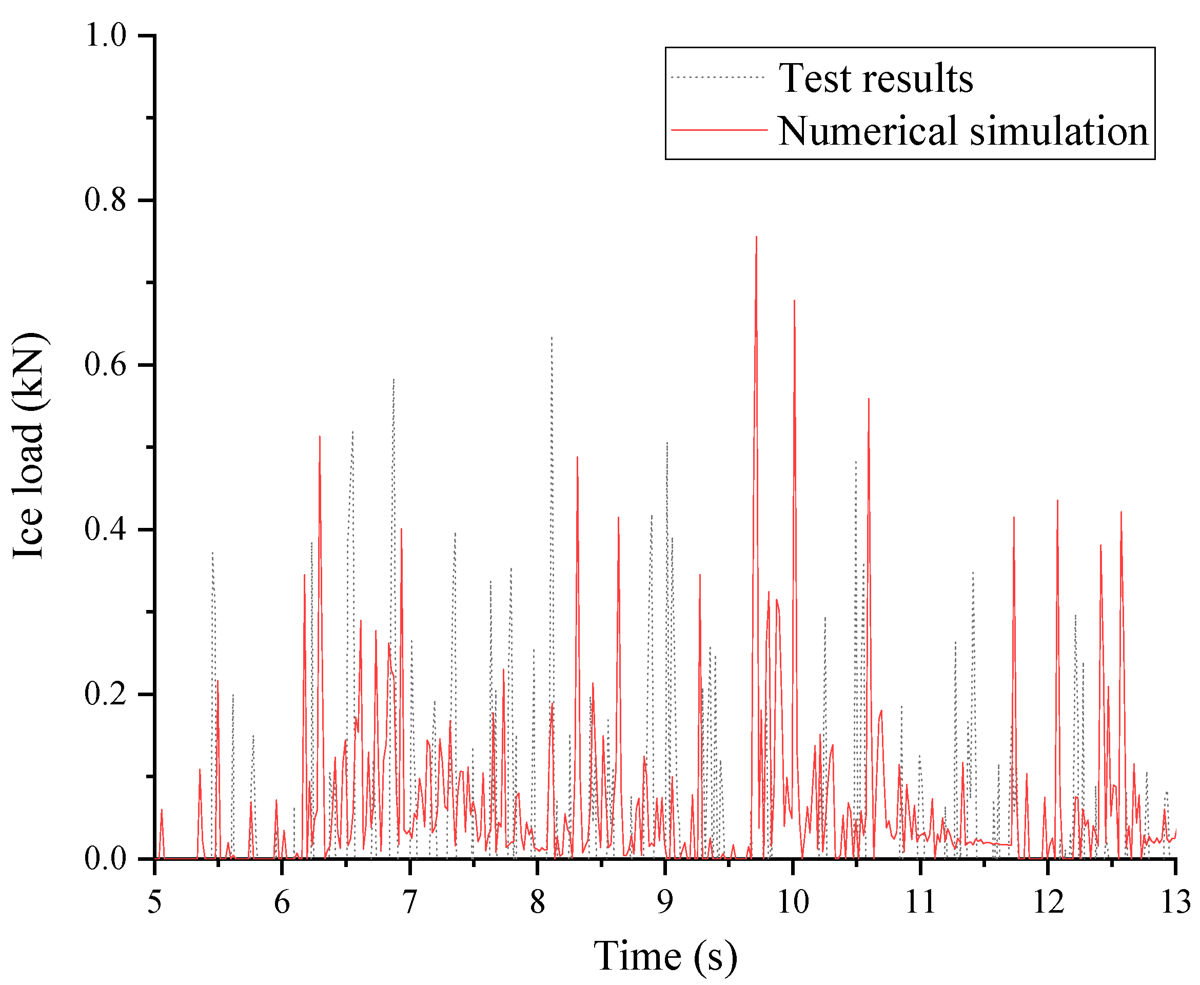
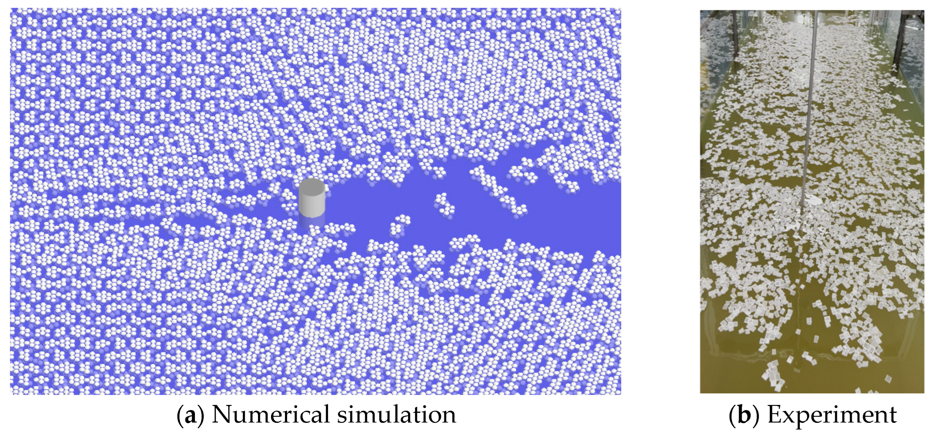
Figure 12 presents a comparative analysis of experimental and numerical simulation results under an ice velocity of 0.05 m/s. The graph reveals that the 5–7 s interval signifies the initial contact between fragmented ice and the structure, indicating a relatively good agreement between the experimental and numerical findings. However, as the contact progressed, a certain degree of deviation emerged between the numerical simulation and experimental results. This discrepancy can be attributed to the inherent randomness in the fragmented ice load, leading to variations in the distribution patterns observed in the experimental and numerical data. Nonetheless, the overall peak loads demonstrated a satisfactory level of correspondence.

Figure 13 depicts the fragmented ice region diagram for both numerical simulation and experimental phenomena. The numerical simulation results consistently aligned with the experimental observations, demonstrating the presence of a relatively open area behind the cylindrical structure with less ice formation. This alignment highlights the accuracy of the numerical simulation method.

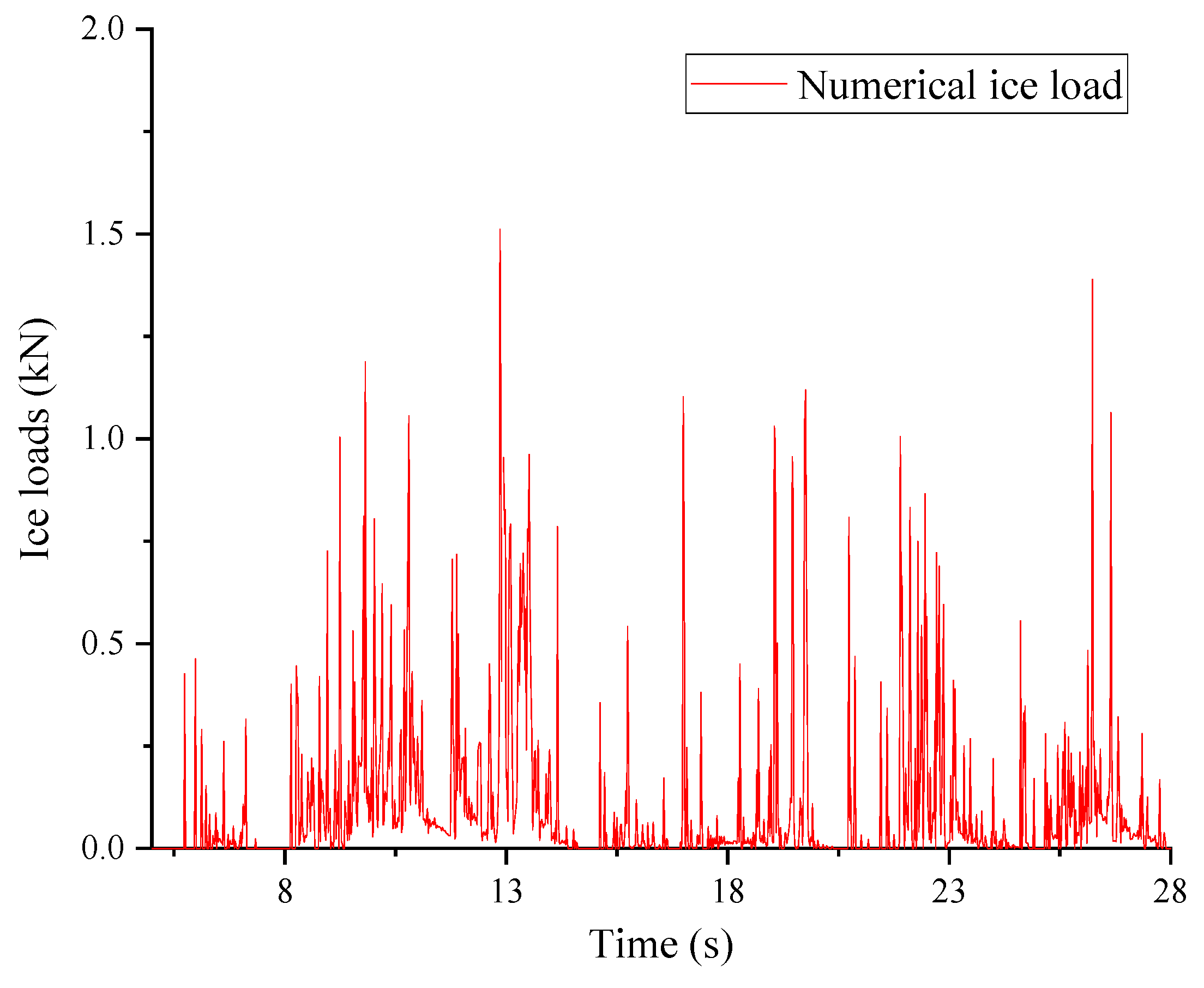
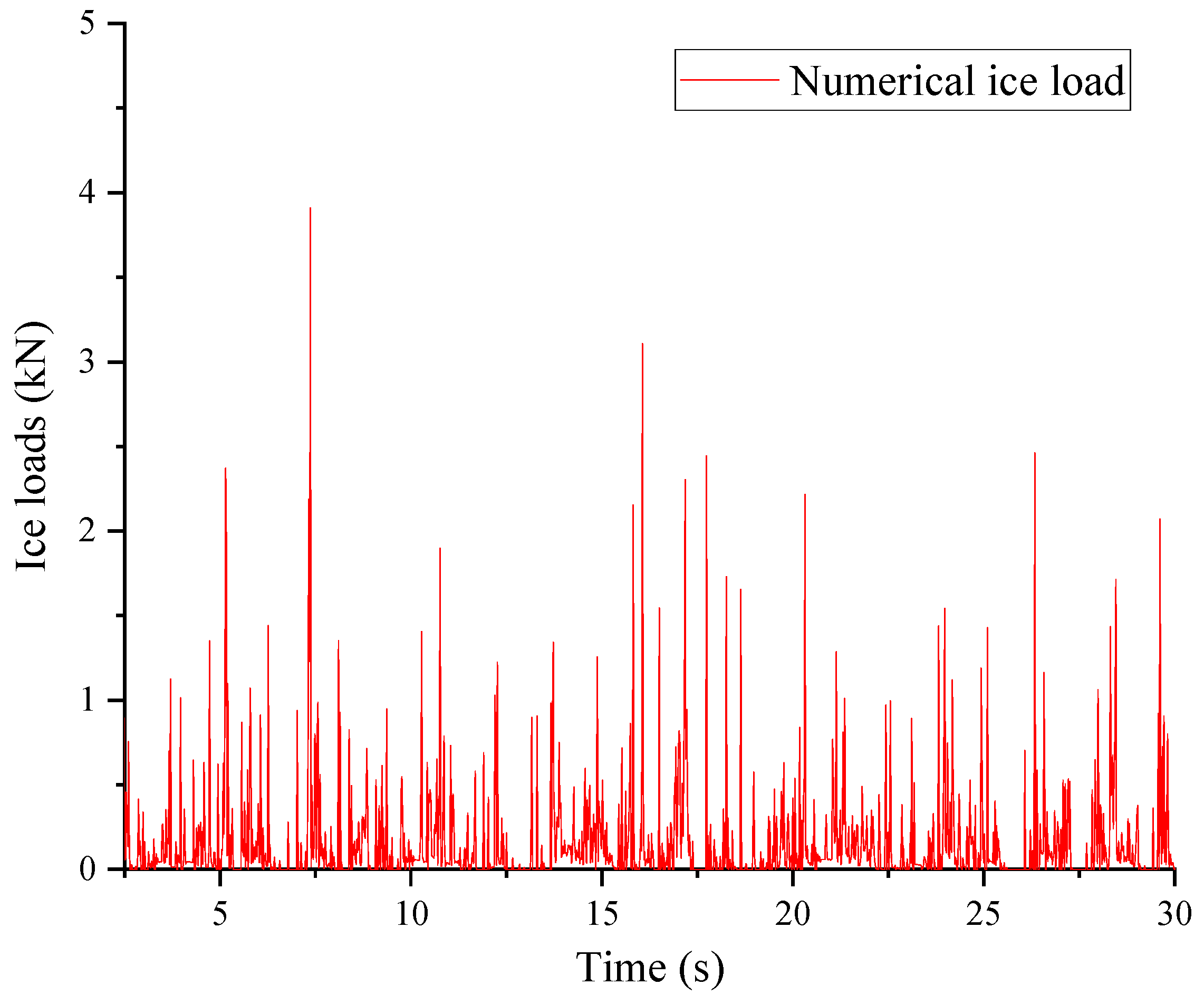
Figure 14 and Figure 15 illustrate the time-domain curves of fragmented ice resistance at ice velocities of 0.075 m/s and 0.125 m/s, respectively. To further validate the accuracy of the numerical simulation method,

Table 5. Statistical values of numerical simulation ice load.

Load Case	Average Ice Load			Significant Ice Load			Max Ice Load
	Test Statistical Result (kN)	Numerical Simulation Statistical Result (kN)	Deviation Ratio	Test Statistical Result (kN)	Numerical Simulation Statistical Result (kN)	Deviation Ratio	Test Statistical Result (kN)	Numerical Simulation Statistical Result (kN)	Deviation Ratio
LC1	0.16	0.17	8.31%	0.36	0.38	6.81%	0.64	0.76	18.13%
LC2	0.47	0.41	12.34%	0.95	0.83	12.63%	1.57	1.51	3.82%
LC3	1.29	1.06	17.83%	2.17	2.39	10.14%	3.95	3.90	1.27%

presents the statistical data on the average ice load, the significant ice load, and the maximum ice load for different ice velocities.

The numerical simulation results demonstrate that the temporal profiles of the overall broken ice loads exhibit significant pulsation characteristics, similar to the experimental results. Under the computational condition of 0.05 m/s, the average, significant, and maximum values of the overall loads were 0.17 kN, 0.38 kN, and 0.76 kN, respectively. These values differed from the corresponding experimental data (0.16 kN, 0.36 kN, and 0.64 kN) by 8.31%, 6.81%, and 18.13%, respectively. Although the maximum load displayed some randomness, the differences between the other stable loads and experimental data were within 10%, indicating a high level of agreement. Under the computational condition of 0.075 m/s, the average, significant, and maximum values of the overall loads were 0.41 kN, 0.83 kN, and 1.51 kN, respectively. These values differed from the corresponding experimental data (0.47 kN, 0.95 kN, and 1.57 kN) by 12.34%, 12.63%, and 3.82%, respectively. All load differences with the experimental data were within 15%, which may be attributed to the vibration on the structure’s surface as the flow velocity increased. Under the computational condition of 0.125 m/s, the average, significant, and maximum values of the overall loads were 1.06 kN, 2.39 kN, and 3.90 kN, respectively. These values differed from the corresponding experimental data (1.29 kN, 2.17 kN, and 3.95 kN) by 17.83%, 10.14%, and 1.27%, respectively. Overall, the load data demonstrated good agreement with the experimental data.

The comparison of the experimental phenomena with the aforementioned computational results reveals that the ice load prediction technique based on the discrete element method can accurately predict ice-breaking patterns and ice loads, and therefore, it has strong potential for practical applications, and the results highlight the effectiveness of the numerical simulation model.

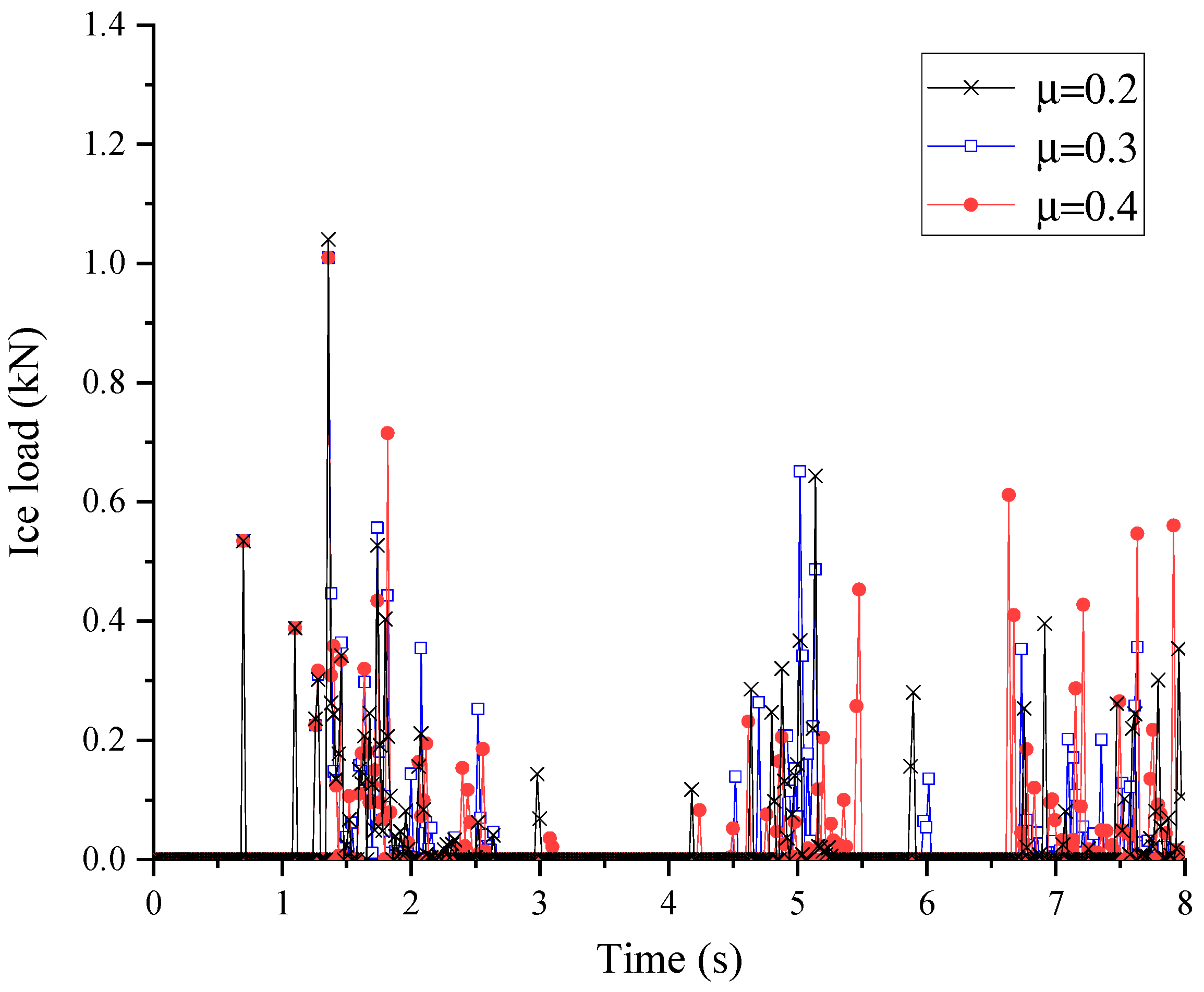
To investigate the influence of the ice friction coefficient on the applied load, we conducted simulations under the conditions of 0.556 m/s ice velocity with friction coefficients of 0.2, 0.3, and 0.4. Figure 16 illustrates the time-history curves of ice fragmentation for each simulation scenario. During the initial stage (0 s~1.5 s), there were minor differences in the ice load among the three cases. However, as time progressed, the movement and contact of fragmented ice varied to different degrees due to random collisions. Consequently, the peak magnitude and occurrence time of the ice load also differed. Overall, when the friction coefficient was 0.4, the applied load was slightly higher, but the difference was not significant. Therefore, further research on ice friction coefficients should consider factors such as ice fragmentation density and ice layer type.

5. Conclusions

This study focused on model experiments and high-performance discrete element methods to investigate the interaction between an upright cylindrical structure and fragmented ice. A comparative analysis was conducted to validate the experimental observations and ice load amplitudes, aiming to explore the mechanisms of interaction between fragmented ice and cylindrical structures. The characteristics of broken ice loads under different ice velocities were analyzed, leading to the following conclusions:

(1)

The fragmentation tests conducted using polypropylene as an ice model material revealed that the broken ice loads exhibited significant temporal randomness, resembling a stable stochastic process. Moreover, the structural broken ice loads demonstrated an increasing trend as the ice velocity increased. These experimental observations closely resemble real-world conditions and provide a more efficient and cost-effective experimental model.

(2)

Through experimental analysis, it was determined that the resistance between broken ice and structures primarily consisted of collision resistance and frictional resistance. By establishing the statistical values for the broken ice resistance coefficient using an average resistance formula, it was observed that this coefficient remained relatively constant across different sailing speeds. This enables the rapid prediction of broken ice loads for specific structures based on the established coefficient.

(3)

The ice resistance obtained from the discrete element method exhibited a strong agreement with the experimental results regarding the distribution pattern of fragmented ice and the statistical values of ice forces. The resistance deviation amounted to approximately 15%. The numerical model demonstrated good applicability in simulating different ice velocities across diverse operational conditions.