Automatic Identification and Suppression of Random Noise and Methods for Profile Splicing in the Sub-Bottom Profile of Deep Water

Abstract

The complex topography of deep sea presents numerous challenges for the accurate exploration of sub-bottom profiles. These include real-time tracking of seafloor reflectors, acquisition and storage of deep-sea long-term reflection data, and splicing of successive profiles. Based on the actual survey data of deep sea, we have developed automatic positioning and noise suppression algorithms, namely the double-difference threshold of proximity points. Furthermore, we have created automatic algorithms, namely content expansion and group data moving, based on extremum in seafloor’s depth. These have been designed to automatically suppress the random noise and effectively splice the sub-bottom profile data in deep water. The aforementioned processing techniques facilitate the enhancement of the quality of deep-water sub-bottom profile data, thereby enabling the provision of a comprehensive and successively long profile for interpretation in the context of deep-water sub-bottom profile data.

1. Introduction

With the increasing access of many countries to the ocean and deep sea, the application of deep-water survey technology is becoming more and more frequent. Acoustic sub-bottom profile is widely used in deep-water sub-seafloor surveying [1,2,3], which can provide an insight into deep-water geomorphological changes and sedimentary spatial distributions, reveal the geological sedimentary processes and geological activities (such as submarine fluid activity, seabed stability, structural activity, etc.), and exhibit a visually successive high-resolution geological cross-section of the seabed for geologists [4,5,6,7,8,9].

Deep-water sub-bottom profiling, compared to the nearshore shallow-water acoustic stratigraphic profiling, encounters many issues, such as insufficient energy, low horizontal coverage, and excessively long propagation records [2]. Insufficient energy can be resolved by combining transducer arrays, and low acoustic horizontal coverage can be mitigated by rapidly and continuously transmitting and receiving signals over short periods. However, the excessively long reflection data pose more challenges in file storage because the standard file storage, such as SEG-Y, has a storage length limit of samples. Currently, the international professional technology in deep-water sub-bottom profile systems typically neglects to record propagation times in the water column and only collects the reflection data within a certain depth range below the seafloor, thereby reducing the amount of data stored. This method resolves the excessively long propagation time, acquires effective data to record in a standard format file, such as SEG-Y, and efficiently saves the storage space. Certainly, this needs a robust algorithm to accurately track the seafloor reflection [2].

The removal of water column propagation should be based on the real-time tracking results of the seabed reflection, which directly affect the quality of the acquired reflection data and the splicing effect of the strata’s reflecting events. As illustrated in Figure 1, the seabed’s reflection curve, which shows its depth, is tracked during acquisition process and serves as the foundation for the subsequent reflection data correction in the deep-water sub-bottom profile. However, there are obvious jumping interference noises in the curve, and it is necessary to find a simple and effective method to suppress these jumping points without destroying the surrounding effective data. In addition, after the reflection data are stored in the SEG-Y format file, the strata’s reflecting events are completely changed, as shown in Figure 2; the seafloor’s reflection becomes completely horizontal, and the sub-seafloor’s strata are also disorganized. As a consequence of these issues, the reflecting events cannot be accurately interpreted, as they are entirely incongruous with the actual seafloor and subseafloor stratigraphy. Therefore, how to effectively splice these strata’s reflecting events of deep-water sub-bottom profile has become an important issue.

Addressing the specific issues encountered in the deep-water sub–bottom surveys, as mentioned above, we developed (1) the automatic positioning and noise suppression algorithms named double−difference threshold of proximity points; (2) the automatic and effective algorithms named the content expansion and group data moving based on extremum in seafloor’s depth; and (3) a method to solve the random noise’s automatic suppression and effective splicing in deep−water sub−bottom profile’s data, as shown in Figure 1 and Figure 2.

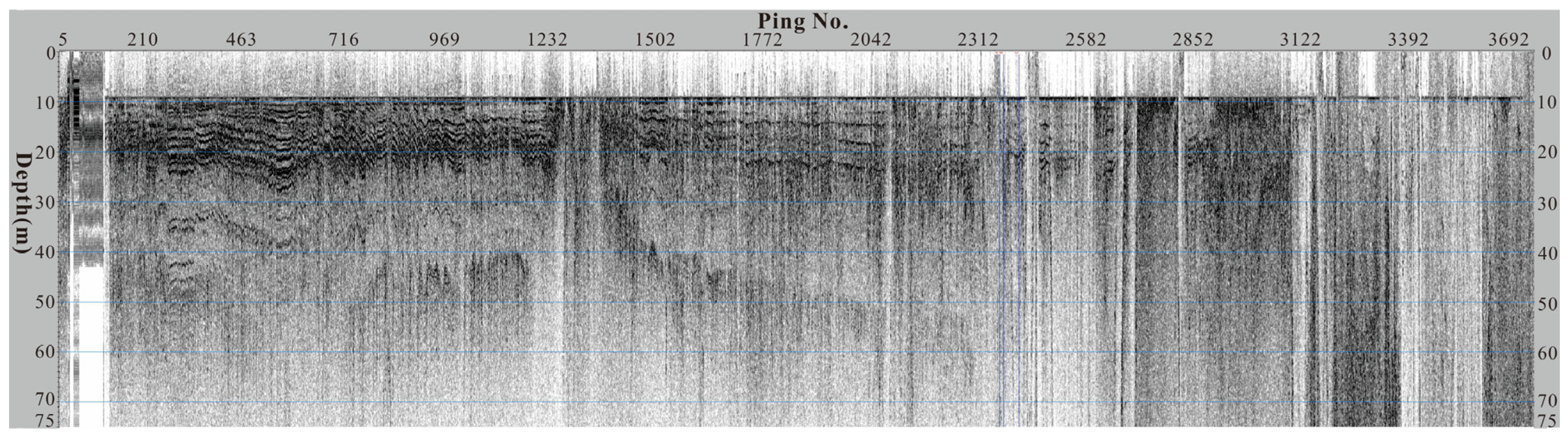
2. Problem Analysis

The principle of deep−water sub−bottom profiling exploration is more advanced than than that of offshore shallow-water acoustic technology. However, there are still some key technical issues that required further development. The first is the conflict between the long-time propagation of acoustic signals in deep water, data recording and storage, and horizontal coverage [2]. Taking the seafloor’s depth of 2000 m as an example, it takes 1.3 s (2000/1500 ≈ 1.3, calculated at the sound’s speed of 1500 m/s) for the acoustic signal transmission to the seafloor by a ship-borne sub-bottom profiler. When the acoustic echo is only reflected from the seafloor, it needs 2.6 s for the two-way propagation (1.3 × 2 = 2.6); considering the two-way propagating time in the sub-seafloor, the recording time of the reflecting signal needs to be more than 3 s. If a high sampling rate is carried out, such as the rate in 32 microseconds, the number of sample points reaches 93,750, which completely exceeds the storage limit of 32,767 points (the limited value of two−byte is 2¹⁵ − 1) in the standard two-byte SEG−Y format. Conversely, the recording length of 3 s necessitates that the interval between the transmission and reception of the acoustic signal exceed 3 s; otherwise, the effective reflected data cannot be received completely. This results in a large horizontal interval between the acoustic signals. If the survey ship sails at the lowest speed of 4 knots, which is equivalent to 2 m/s, the horizontal interval between the acoustic signals will reach 6 m. A large interval will make the horizontal coverage of the signal on the seabed too sparse, resulting in poor horizontal resolution and poor continuity in the reflecting strata’s events of the sub-bottom profiler. The deeper the water depth, the larger the transmission interval, and the lower is the acoustic horizontal coverage; if the ship’s speed is faster, the horizontal coverage is lower. In order to solve these problems, the international mature instruments adopt multi-ping’s short-time continuous transmission and synchronous reception and employ the method of removing the propagation data in the water column to decrease the samples during acquisition so as to attain the continuous transmission and reception of the acoustic signals in a short time and match the storage limit of the SEG-Y format file.

To remove the acoustic wave propagating data in the water column, it is necessary to perform the real-time tracking of the seafloor’s reflection and save the tracking results into the SEG-Y file’s definition during acquisition. Based on the real-time tracking results, the acquisition system automatically removes the acoustic propagation data in the water column above the seabed and only saves the effective reflection data below the seabed, thereby reducing the recording time and the amount of stored data. Additionally, there exist two other problems: first, the accuracy of the tracking results of the seabed’s reflection determines whether the seafloor’s reflection data are correctly acquired; and second, the reflection data stored in the SEG-Y format require re-stitching, as shown in the original profile in Figure 2. During field data acquisition, real-time tracking of the seabed’s reflection can be subject to various interfering factors, such as sea conditions causing the survey vessel to sway, the acoustic wave’s transmitted angle, sensitivity of the deep-water sub-bottom profiler, and field parameter settings during acquisition. These interferences can lead to incorrect seabed’s reflection tracking results, as indicated by the jumping points in Figure 1. These jumping points usually require manual elimination and the profiler’s correction processing. Traditional methods, such as the sliding average method [7,10], median filtering method [11,12], and polynomial fitting method [13,14,15], can only correct jumps at single points or a few consecutive points, but they cannot correct the block-wide multi-jumping points in tracking results. The correction process may also destroy the valid data near the jumping points, introducing errors in the subsequent profile-splicing process. After effectively correcting the real-time tracking results of the seabed’s reflection, it is also necessary to perform the reflection events’ stitching on the reflection profiles stored in SEG-Y format. Otherwise, the original profile, as shown in Figure 2, cannot reveal the real topography and sedimentary structure. Developing a simple and reliable method to effectively stitch these large-volume reflections’ data is also a challenge.

3. Problem Solution

In order to solve the above issues, there are two fundamental problems that need to be addressed in the deep-water sub-bottom profile’s survey: first, the elimination of irregular jumping points in the real-time tracking of the seabed’s reflection during acquisition; and second, the effective stitching of the reflecting events in profiles after removing the acoustic traveling time in water columns. For the first problem, we developed an automatic positioning and noise suppression algorithm named the double-difference threshold of proximity points, which can automatically locate the jumping points and compute an effective substitute value within the proximity points. For the second problem, we provide algorithms named the content expansion and group data moving based on extremum in seabed’s depth to automatically splice the reflecting events.

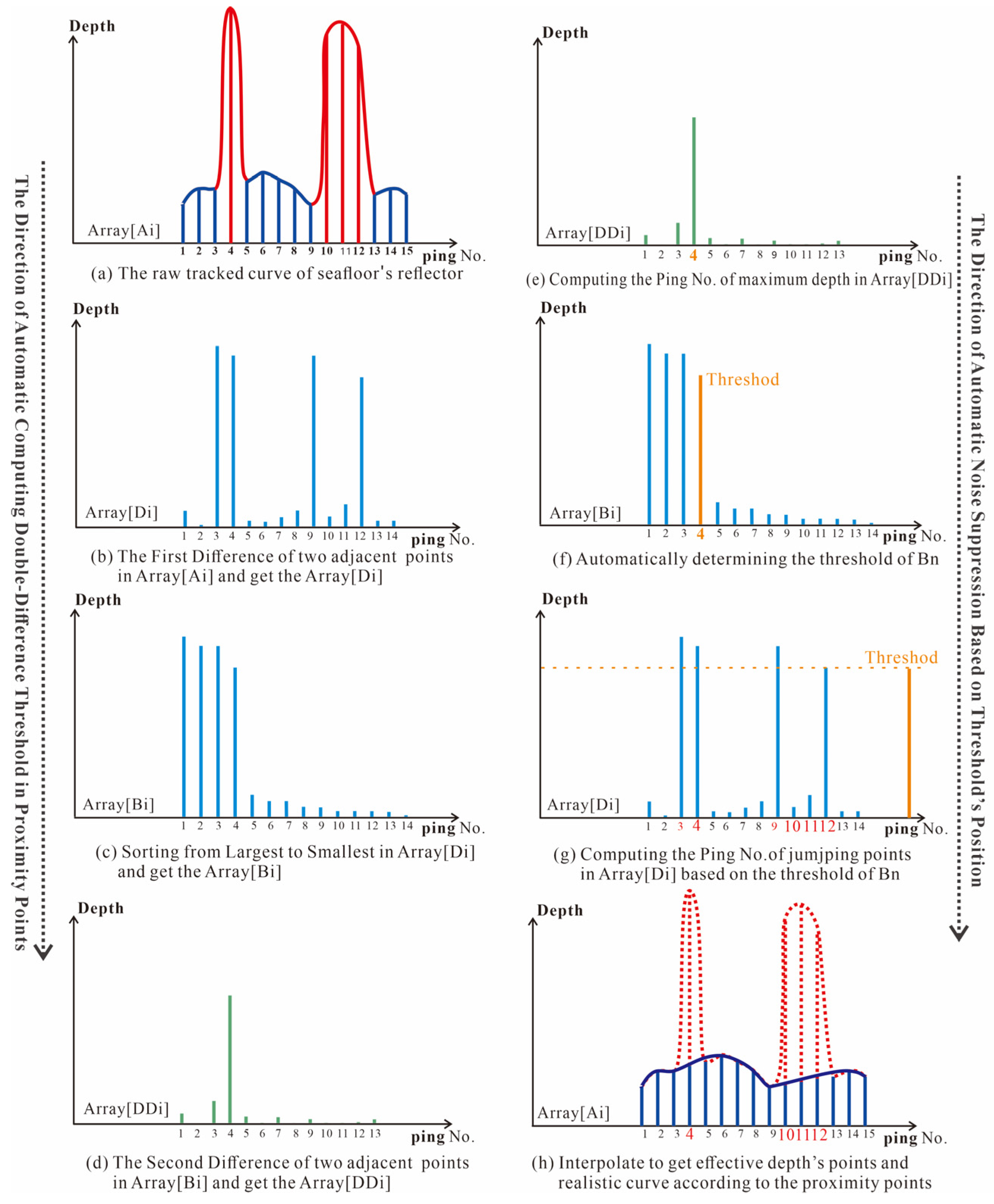
3.1. Algorithm of Proximity Points’ Double-Difference Threshold

By computing two adjacent points’ difference twice, this method obtains the difference distribution of all the points, eliminates the relevant background value with difference computing, and then gets an obvious abnormal characteristic point through sorting. This enables the algorithm to automatically identify the jumping threshold following the two distinct calculations, back−calculate the distribution position and serial number of the jump points, and then perform the corresponding correction process. The principle of this method is shown in Figure 3, and the automatic calculation process is divided into two parts. Firstly, the double difference of proximity points is calculated to automatically find out the abnormal jumping value’s threshold, which is divided into three steps (the left part in Figure 3). Step a represents the original tracked depth curve of the seafloor’s reflector. There are two errors in tracking the jumping points denoted with red lines on the curve: one is a single jumping point and the other is a continuous multi-points jump. The original data are stored in computer memory array A_i. Step b indicates that the first difference operation is performed on the original data A_i to generate a new array D_i. The first difference operation basically eliminates the normal background value and highlights the outlier of the jumping point. In Step c, the primary difference array D_i is sorted from the largest to the smallest, generating the array B_i. The sorting process is meant to prepare for the subsequent secondary difference and provide a new dataset to compute the existence of multiple outliers and further suppress the remaining background values. In Step d, the second difference operation is performed based on the first difference result B_i after sorting, thus obtaining a new array DD_i. The DD_i is once more calculated based on the initial difference of two consecutive points. Given that there is only one jumping point and the background value in the array DD_i is minimal, the interference factor for automatic judgement is essentially eliminated. At this time, the corresponding sequence number of the jumping point can be back-calculated according to a single maximum jumping position.

After obtaining the single prominent abnormal jumping point through the above double-difference calculating process, the following threshold’s judgment and automatic positioning calculation are performed on the right side of Figure 3, which is equivalent to the reversing calculation of the process on the left side of Figure 3. Starting from the position of the single maximum value in the double-difference (step e), the corresponding jumping point position is deduced by reversing the single-difference threshold and sorting Bi, thereby obtaining the jumping threshold after single-difference sorting (step f). Using this threshold, all jumping points and their corresponding positions in the D_i array can be identified (step g). Through locating these jumping points’ positions, the corresponding abnormal points’ positions in the original data A_i can be deduced. It is important to note the matching of element sequence numbers between A_i and D_i arrays, as the subtraction operation in A_i reduces the number of members in D_i by one, correspondingly reducing the count of jumping points. Furthermore, the automatic identification and suppression of jumping points in the original data A_i can be performed, and the jumping point is replaced by linear interpolation in proximity values (step h), obtaining the final reliable correction result.

The formula for calculating the threshold’s value on the left side of Figure 3 is as follows:

$$\begin{array}{l}{\mathrm{D}}_{\mathrm{i}}={\mathrm{A}}_{\mathrm{i}+1}-{\mathrm{A}}_{\mathrm{i}};\\ {\mathrm{B}}_{\mathrm{i}}=\mathrm{SORT}({\mathrm{D}}_{\mathrm{i}});1\le \mathrm{i}<\mathrm{N}\\ \mathrm{D}{\mathrm{D}}_{\mathrm{i}}={\mathrm{B}}_{\mathrm{i}+1}-{\mathrm{B}}_{\mathrm{i}}\end{array}$$

(1)

In Formula (1), D_i is the result of the first difference in the raw adjacent points, B_i is the sorting result of D_i from large to small, and DD_i is the result of the secondary difference in B_i. After the twice-difference calculation, the background value of the original points is further reduced. Multiple jumping points are reduced to a single point, which provides the key for automatically calculating the threshold. With the DD_i result, the inverse calculation can be carried out. The inverse calculation mainly uses the position of the single largest jumping point after the double difference operation corresponding to the arrays B_i and D_i and then automatically obtains the position and number of the jumping points in the original array A_i. Because the internal subtraction operation of array elements will reduce the array elements by one in a new memory array, there are two fewer elements than the original data after the twice-subtraction operation; therefore, during the inverse operation, special attention needs to be paid to the number of array elements, and the corresponding position sequence in the array needs to be accurately computed; that is the key to correctly judging the abnormal jumping points.

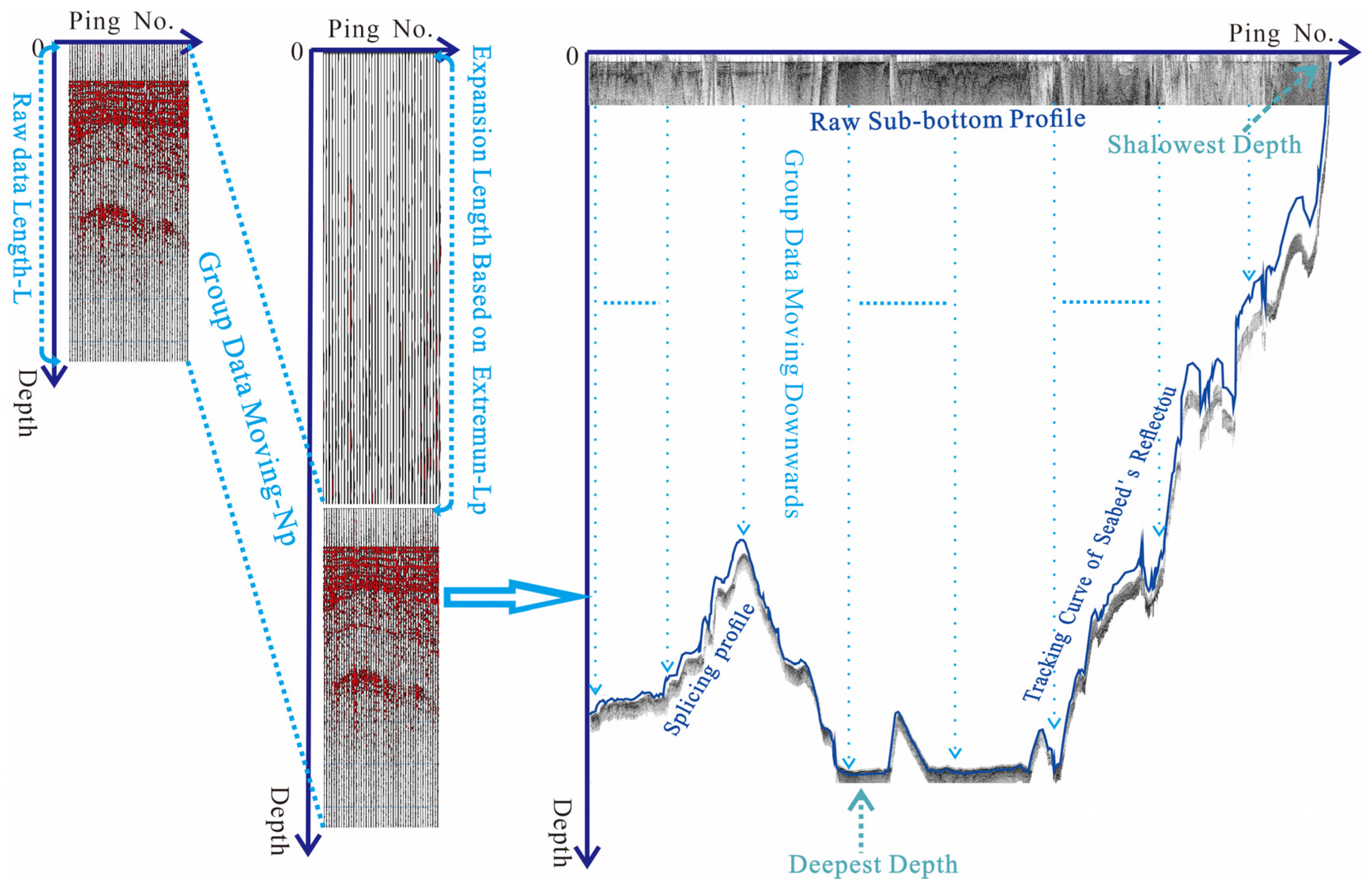
3.2. Algorithm of Content Expansion and Group Data Moving Based on Extremum in Seabed’s Depth

After completing the jumping points’ suppression in the tracked seafloor reflection curve as described above, it is also necessary to splice the strata reflection’s events in the SEG-Y data. The algorithmic basis of the splicing processing is to move the data bodies in groups, similar to the dynamic correction processing in multi-channel seismic. However, the complex topography of the deep-water seafloor, such as many reefs and shoals, crisscross troughs, and steep and long seamounts, which cause changes from hundreds of meters to several kilometers in topography, introduces great challenges to the data bodies’ moving and profile imaging in deep-water sub-bottom profiles.

Due to the sample range limit of the SEG-Y format file, it is inevitable that the moving of data bodies will exceed the range limit. In Figure 1, the shallowest part is less than 700 m, while the deepest part exceeds 3700 m; the sub-bottom profile’s data need a recording length of 8000 samples from 700 m to 3700 m. With such a large span of water depth, the conventional group moving method will definitely cause the memory array to go out of bounds and cause memory leakage errors.

To solve this problem, we need to effectively expand the array capacity to get enough storage space for the group data migration. If the memory expansion is not enough, a memory leak will occur when the group moves, while if the expansion is too much, it will cause a waste of storage space and even a system crash. After continuous research, we used the corrected seafloor reflection curve to set the expansion size with the extremum in seafloor depth, effectively manage the overhead of storage space and the range of moving in groups, ensuring the integrity of the splice profile.

The calculation formula is as follows:

$$\begin{array}{l}{\mathrm{L}}_{\mathrm{p}}={\displaystyle \frac{({\mathrm{D}}_{\max }-{\mathrm{D}}_{\min })}{(\mathrm{v}\times \mathrm{sp})}}-\mathrm{L}\\ {\mathrm{N}}_{\mathrm{p}}={\mathrm{R}}_{\mathrm{track}}-{\mathrm{R}}_{\mathrm{raw}}\end{array}$$

(2)

In Formula (2), D_max and D_min respectively, represent the deepest and shallowest depth after correction of the seabed’s reflection curve, v represents the sound velocity in water, sp represents the sampling rate, L represents the original recording length of the SEG-Y file, and the result of L_p is the optimal array capacity that needs to be expanded for group moving. R_track and R_raw respectively, represent the seabed’s reflection position on the current seabed’s tracking depth and the original depth in the SEG-Y recording file, and N_p is the offset that needs to be moved in the current group data moving. After the current Ping’s data move the offset of N_p backward, the amplitude data point at the vacant position is filled with zero. With the same processing, all the Ping’s group moving is completed, and a reliable deep-water sub-bottom profile is finally obtained.

This formula’s algorithm is illustrated in the schematic diagram in Figure 4.

3.3. Processing Flow

The process proposed in this paper based on the algorithms mentioned above, is shown in Figure 5. First of all, it is necessary to obtain the seafloor’s reflection curve tracked upon acquisition from the SEG-Y recording file, draw the corresponding curve after reading the storage’s data, and then implement the automatic positioning and suppression algorithm of double-difference threshold to proximity points. The key of this algorithm is the accurate calculation of threshold values and the effective judgment of the location in jumping noise. The purpose of the twice-difference calculation of proximity points in the algorithm is to fully eliminate background values in all points and highlight the amplitude of abnormal jumping points, which can provide a basis for accurately computing threshold values. After the effective correction of the seafloor reflection curve, another algorithm of content expansion and group data moving is carried out, which is based on the maximum and minimum in the seafloor’s depth, thus effectively splicing the sub-bottom profile to obtain successive reflective events. The detailed process is shown in Figure 5.

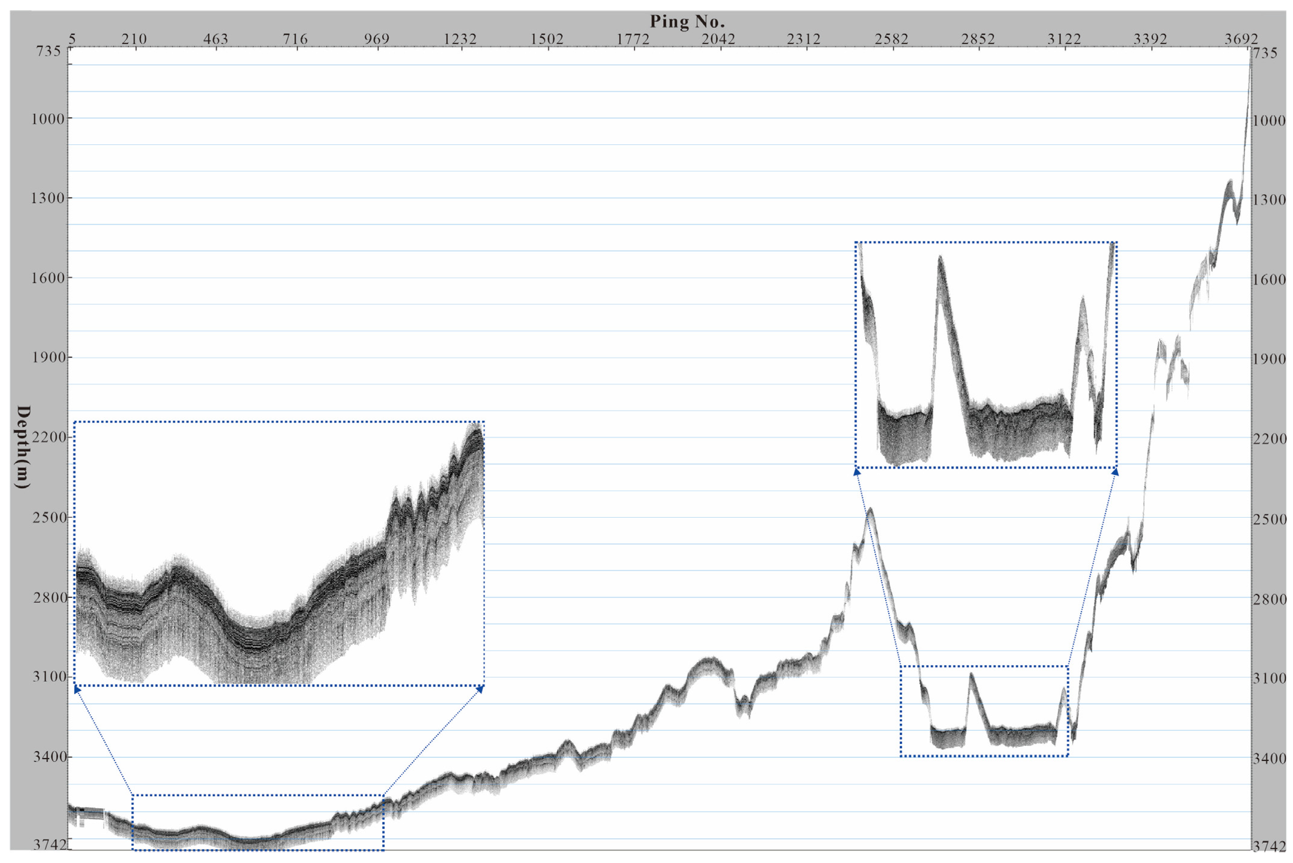
4. Processing Results

Based on the method mentioned above, we have programmed the algorithms to automatically process the sub-bottom profile of deep water, as shown in Figure 1 and Figure 2, and verify the effectiveness of the proposed method. The deep-water sub-bottom profile data were collected using the Bathy-2010 system from the American company SyQwest. In Figure 1, the tracked seafloor’s depth reaches a maximum of 3692 m and a minimum depth of about 740 m. The depth curve exhibits three distinct jumping noises: the first is a continuous and group jumping noise, with a total of over 100 consecutive points, indicating a block-wide depth’s tracking error; the second is a continuous tracking error over 3 jumping points; and the third is a single jumping point’s tracking error. The errors in the second and third cases, involving only a few points, are generally easier to handle, while the first case of extensive group continuous multi-jumping points is typically more challenging to suppress. Using the algorithm of proximity points’ double-difference threshold to automatically position jumping points and compute the reasonable substitution, the results are shown in Figure 6. From the results, it can be seen that all the jumping points were effectively suppressed, and the depth’s curve is successive, which is consistent with the real seabed’s depth compared with multi-beam depth.

Using the corrected reflection curve of the seafloor, the corresponding extremum in the seabed’s depth can be found. The deepest depth in the curve is 3692 m, and the shallowest depth is 735 m. The contents of each Ping’s data array are expanded from the original 8000 to 79,070 points based on the difference between the deepest and shallowest depth. After memory expansion, the group moving operation was completed according to the calculated offset. The final result is shown in Figure 7. The reflective profile in the figure is basically consistent with the actual topography, and the sedimentary strata’s reflections in the trench and the basin are rich; each reflective event as shown in the two enlarged sub-bottom profiles is continuous and consistent.

5. Conclusions

Deep-water sub-bottom profiling is widely used in deep-sea geological and geophysical surveys. Affected by the abrupt changes in the topography of the deep sea, the depth of the seafloor jumps from several hundred meters to several thousand meters, which poses many challenges to sub-bottom profiling. Obvious problems include the real-time tracking of seafloor reflections and data storage. Real-time tracking in the field is susceptible to various disturbances, such as sea conditions, instrument sensitivity, and parameter settings, resulting in poor acoustic tracking of the seafloor reflection and introducing jumps in the tracking curve, which further affect subsequent profile splicing. Therefore, the raw data from the deep-sea sub-bottom profiles need to be further processed, while the relevant technology application is lacking at present.

Based on the actual deep-sea sub-bottom profile data, we discuss how to effectively suppress jumping points in the seafloor reflection curve and how to effectively splice the reflection profile. In this regard, we have made the following contributions:

(1)

We developed the algorithm of proximity points’ double-difference threshold to automatically position and suppress the jumping points; then we used this algorithm to accurately suppress the random noise.

(2)

We introduced the algorithms of the content expansion and group data moving method based on extremum in seafloor depth; then we used these algorithms to effectively splice the sub-bottom profile data.

Both methods are fully automated by the algorithm modules without any manual parameter intervention. With these methods, we have processed more than 50,000 km of sub-bottom profile data distributed in the South China Sea, the Pacific Ocean, and the Polar region. The methodologies presented in this paper provide a technical foundation for the professional processing and subsequent geological interpretation of deep-water sub-bottom profiles.

It is evident that any algorithm must undergo continuous validation and refinement across a diverse range of practical applications. In light of the intricate topography and evolving sub-bottom profile observed in deep-water environments, it is imperative to regularly update the algorithm and develop novel techniques, such as precise recognition in the presence of noise, through the utilization of fully intelligent and high-resolution processing technology in sub-bottom profiling.

References

- Yang, G.; Zhu, J.; Zhao, D.; Xiong, Z.; Wang, C.; Ou, X.; Jia, Y.; Li, S. Development and application of sub-bottom profiler technologies. Mar. Sci. 2021, 45, 147–162. (In Chinese) [Google Scholar]
- Ding, W.; Li, J.; Su, X.; Zhang, J.; Jiang, W.; Han, F. Technology research and development for acoustic sub-bottom survey in deep sea. Acta Oceanol. Sin. 2015, 37, 70–77. (In Chinese) [Google Scholar]
- Zhu, J.; Zhou, T.; Li, T.; Chen, B.; Meng, X.; Mazhar, S. High-resolution sub-bottom profiling technology using parametric array and vector hydrophone. Appl. Acoust. 2024, 223, 110077. [Google Scholar] [CrossRef]
- Gutowski, M.; Bull, J.M.; Dix, J.K.; Henstock, T.; Hogarth, P.; White, P.R.; Leighton, T.G. Chirp sub-bottom profiler source signature design and field testing. Geophys. Res. Abstr. 2002, 23, 481–492. [Google Scholar] [CrossRef]
- Gutowski, M.; Bull, J.M.; Dix, J.K.; Henstock, T.; Hogarth, P.; White, P.R.; Leighton, T.G. Design of a 3D Chirp Sub-bottom Imaging System. Mar. Geophys. Res. 2005, 26, 157–169. [Google Scholar]
- Anderson, N.; Alotaibi, A.M. Site Assessment Using Echo Sounding, Side Scan Sonar and Sub-Bottom Profiling; A National University Transportation Center at Missouri University of Science and Technology, Tech Report; February 2014; Available online: https://ntlrepository.blob.core.windows.net/lib/52000/52700/52710/R338_Final_Report.pdf (accessed on 10 November 2024).
- Kim, Y.-J.; Koo, N.-H.; Riedel, M.; Namgoong, H.; Lee, J.-M.; Cheong, S.; Joo, Y.; Yoo, D.-G.; Chun, J.-H.; Lee, H.-Y. A case study on swell correction of Chirp sub-bottom profiler (SBP) data using multi-beam echo sounder (MBES) data. J. Appl. Geophys. 2017, 145, 100–110. [Google Scholar] [CrossRef]
- Zhang, C. Fractal analysis of muddy submarine channel slope instability from sub-bottom profile images. Mar. Georesources Geotechnol. 2021, 40, 701–711. [Google Scholar] [CrossRef]
- Gutowski, M.; Bull, J.M.; Dix, J.K.; Henstock, T.J.; Hogarth, P.; Hiller, T.; Leighton, T.G.; White, P.R. Three-dimensional high-resolution acoustic imaging of the sub-seabed. Appl. Acoust. 2008, 69, 412–421. [Google Scholar] [CrossRef]
- Luo, J.; Pan, G.; Ding, W. Research on processing technique of eliminating wave-induced distortion effect on sub-bottom profile. Tech. Acoust. 2009, 28, 21–24. (In Chinese) [Google Scholar]
- Wu, J.; Li, C.; Zhou, W. Comparison between the Noise suppressing Abilities of the Median Filters and the Average Filters. J. Nanchang Univ. Eng. Technol. 1998, 20, 32–34. (In Chinese) [Google Scholar]
- Ding, W.; Feng, X.; Fu, X.; Gou, Z.; Wei, Y. Marine wave correction research on single channel seismic data and sub-bottom profile. Acta Oceanol. Sin. 2012, 34, 91–98. (In Chinese) [Google Scholar]
- Amri, U. Recent Sediment Analysis, Study Case: Sub Bottom Profiler Data Line 8 Geomarine Research Vessels. J. Wetl. Environ. Manag. 2019, 7, 123. [Google Scholar] [CrossRef]
- Zhang, J.; Gan, X.; Zhou, Z.; Yang, J. 4D track prediction of aircraft based on improved sliding window polynomial fitting method. Adv. Aeronaut. Sci. Eng. 2019, 10, 601–608. (In Chinese) [Google Scholar]
- Saleh, M.; Rabah, M. Seabed sub-bottom sediment classification using parametric sub-bottom profiler. NRIAG J. Astron. Geophys. 2016, 5, 87–95. [Google Scholar] [CrossRef]
Disclaimer/Publisher’s Note: The statements, opinions and data contained in all publications are solely those of the individual author(s) and contributor(s) and not of MDPI and/or the editor(s). MDPI and/or the editor(s) disclaim responsibility for any injury to people or property resulting from any ideas, methods, instructions or products referred to in the content. |
© 2024 by the authors. Licensee MDPI, Basel, Switzerland. This article is an open access article distributed under the terms and conditions of the Creative Commons Attribution (CC BY) license (https://creativecommons.org/licenses/by/4.0/).
Share and Cite
Feng, X.; Ding, W. Automatic Identification and Suppression of Random Noise and Methods for Profile Splicing in the Sub-Bottom Profile of Deep Water. J. Mar. Sci. Eng. 2024, 12, 2069. https://doi.org/10.3390/jmse12112069
Feng X, Ding W. Automatic Identification and Suppression of Random Noise and Methods for Profile Splicing in the Sub-Bottom Profile of Deep Water. Journal of Marine Science and Engineering. 2024; 12(11):2069. https://doi.org/10.3390/jmse12112069
Chicago/Turabian StyleFeng, Xia, and Weifeng Ding. 2024. "Automatic Identification and Suppression of Random Noise and Methods for Profile Splicing in the Sub-Bottom Profile of Deep Water" Journal of Marine Science and Engineering 12, no. 11: 2069. https://doi.org/10.3390/jmse12112069
APA StyleFeng, X., & Ding, W. (2024). Automatic Identification and Suppression of Random Noise and Methods for Profile Splicing in the Sub-Bottom Profile of Deep Water. Journal of Marine Science and Engineering, 12(11), 2069. https://doi.org/10.3390/jmse12112069