Study on Spatial Scale Selection Problem: Taking Port Spatial Expression as Example

Abstract

Spatial scale is a key factor, which affects the accuracy of spatial expression and further influences the spatial planning of a research area. In order to help improve the efficiency and accuracy of optimal scale selection for all sizes of research areas, a universal two-layer theoretical framework for optimal scale selection was proposed in this paper. Port area was taken as an example to systematically clarify the application of the proposed framework, and the scale selection model for port spatial expression was established. Least-squares-based mean change point analysis was introduced into the model, and the concept of a comprehensive change point was proposed to form the criterion for optimal port scale selection. First, an appropriate scale domain was preliminarily determined by the upper scale selection model. Then, the lower scale selection model determined the final appropriate scale domain and took the corresponding scale of a minimum comprehensive change point as the final optimal scale for port spatial expression. Finally, a port area in Qingdao in eastern China was taken to verify the feasibility of the proposed model, and the optimal scale was suggested to be 14 m. The proposed framework in this paper helps ensure the accuracy of spatial expression and reduce spatial data redundancy, and it can provide the methodological references for planners to better spatialize a research area, which will guarantee the subsequent spatial planning work.

1. Introduction

Spatial scale is a fundamental concept to geography [1]. Changes in the spatial scale will lead to variations in the spatial attribute information [2,3], which will directly affect the accuracy of spatial expression and indirectly influence spatial characteristics analysis and spatial function planning. This further confirms the importance of spatial scale to spatial research. Therefore, how to select an appropriate scale for the spatial expression of a research area is the key problem to be solved before carrying out any spatial research [4].

The scale problem widely exists in many research disciplines. Relevant research works cover subjects including terrain and geomorphology [5,6,7], ecology and climate [8,9], environmental pollution [10], land use [11,12], social population [13], etc. Studies on scale transformation [14,15], scale effect analysis [16,17] and optimal scale selection [18,19] occupy the main part of scale-related research. The realization of scale transformation lays a data foundation for scale effect analysis and optimal scale selection, while the analysis of the scale effect provides a decision basis for the selection of optimal scale. There is no single spatial scale suitable for all research objects [20], and the appropriate scale may even be different for the same geographic object according to various research purposes.

Spatial scale has always been a focus in remote-sensing studies. Scholars have discussed the scale effect of land cover classification from multi-resolution data and proposed the determination method for an appropriate scale [4,21,22,23]. For example, Ming et al. [22] proposed a modified average local variance (ALV) method to select the optimal spatial resolution for image classification. With regard to geographic data, indicators like local variance (LV) and the rate of change in LV (ROC-LV) [5], width functions and area functions [6], the number of rills and the average length of rills [7] were chosen to carry out multi-scale analysis and analyze the scale effect of geomorphological features. Liu et al. [10] explored the multi-scale effects of anthropogenic activity influences on groundwater nitrate contamination, and the corresponding spatial scale of the highest scaling correlation was suggested to be the optimal scale. Guo et al. [24], Scammacca et al. [25] and Wu et al. [26] carried out multi-scale analyses on soil data to reveal the scale effect of soil. Moreover, land use and land cover data also have a certain dependence on spatial scale. Some researchers discussed the modifiable areal unit problem and carried out scale effect analyses on the landscape pattern [11,27,28]. In order to determine the optimal scale for analyzing the landscape pattern of a research area, methods like landscape metrics analysis, the coefficient of variation method, information loss model, etc. were often applied [12,18,19,29]. Moreover, Cao [30] and Wang et al. [31] took indicators like the continuity degree, Gini coefficient, urban expansion rate, etc. to analyze the scale effect of urban spatial features. For research on arable land use changes, methods like the landscape metric and spatial regression analysis [32], spatial autocorrelation and scale variance analysis [33], principal component analysis [34], etc. were employed to carry out the multi-scale analysis. In studies on the relationship between landscape patterns and land surface temperatures, multiple landscape metrics were applied to conduct scale effect analysis [8,9,35,36]; for example, Liu and Weng [8] discussed the scale effect via landscape metrics analysis and determined the optimal resolutions based on the minimum distance in the landscape metric spaces. To find out the optimal spatial scale for analyzing landscape ecological risk changes, Ai et al. [37] and Wang et al. [38] both carried out semi-variogram analyses and analyzed the landscape pattern. When it comes to socio-economic data, Huang et al. [13] proposed an improved average local variance method for evaluating grid size suitability for expressing the discrepancies in population density. Chen et al. [39] proposed a semi-variogram-based method to quantitatively evaluate the scale effect of extensive data.

In summary, carrying out a quantitative analysis on the scale effect by analyzing the relationship curve between scale and analysis indices (scale–index curve) and further determining the optimal scale by observing the turning location of the curve has been a universal method for studies on the scale effect and optimal scale selection. Furthermore, it can also be found that the size of a research area varies a lot, e.g., a city, a province or even a larger region. In some literature works [38], when the size of a research area is relatively large, the interval of the scales used for scale effect analysis is accordingly set to be large. This may miss the variation characteristics of analysis indices at small scales and thus influence the determination of an optimal scale.

In order to help improve the efficiency and accuracy of the scale selection process for all sizes of research areas, this paper proposes a two-layer theoretical framework for optimal scale selection. Here, the spatial scale is defined as a spatial resolution, which represents the size of the grid. The two-layer framework involves two analysis layers, which are separate under the scales of different intervals, and the upper layer can help quickly locate an appropriate preliminary scale domain, while the lower layer can then further determine the final optimal scale.

It is obvious that the multi-scale analysis of scale–index curves and the criterion for optimal scale selection are two significant bases for the proposed framework to determine the final optimal scale. The analysis indices used for scale effect analysis and optimal scale selection in related research works involve landscape metrics [8], spatial autocorrelation index [33], local variance [5], etc. Reasonable analysis indices are of great significance to the subsequent scale effect analysis and scale selection process. Thus, this paper chose a group of corresponding landscape metrics from three perspectives as quantitative analysis indices to conduct a multi-scale analysis on the spatial features of every land use function in order to comprehensively evaluate the expressivities of component information, configuration information and spatial distribution information of all land use functions in the research area. Meanwhile, in the existing literature [40,41,42], the analyses of scale–index curves and observations of turning locations have often been conducted via visual interpretation, which is subjective to some extent and lacks accurate mathematical basis. This may bring errors when the variation tendency of the curve is complex. In order to improve the accuracy of the analysis process, change point analysis was added into the two layers of the framework to analyze the variation tendencies of scale–index curves more comprehensively and objectively compared with the traditional whole-process visual observation method. Change point analysis can quantitatively detect the abrupt changes in a data series and has been widely applied in fields like statistics and signal processing [43], financial analysis [44], climate analysis [45], flood analysis [46], etc. In this paper, a least-squares-based mean change point analysis method was introduced into two layers to detect the change points of a scale–index curve. Furthermore, based on the detected change points, this paper proposes a comprehensive change point analysis method to calculate the overall turning location of the curve and help determine the final appropriate scale domain. Then, the criterion for the final optimal scale selection in the lower layer is proposed according to the requirement of the research area to determine the final optimal scale.

This paper looked at scale selection in a port area as an example to specifically clarify the proposed framework. Ports are located at the junction of land and ocean, and they involve components like vessels [47,48], berths [49], yards [50] and many other facilities. Ports are important nodes of logistic transportation chains [51,52], and they closely relate to the urban economy and residential living environment. Therefore, port spatial planning is of great significance for the development of a city. In order to ensure the smooth progress of port spatial planning, the primary task is to accomplish the spatial expression of the whole port based on port spatial data, which are the basic data for statistical analysis of port spatial features and research of port spatial planning. Therefore, the framework proposed above was applied to select the optimal scale to accomplish the spatial expression of port functions.

The spatial features of a port area are special to some extent. First, the spatial extent of a port area is quite small (as shown in Figure 1). From the perspective of geographical location, compared with the adjacent city area and ocean area, the port area is relatively small. From the perspective of land width, the land width of a container terminal is about 500~1200 m, while the land width of a general cargo terminal is about 100~600 m [53], which is relatively small. Second, the port area has high requirements for spatial expression (as shown in Figure 2). The development of a port follows detailed planning arrangements, and the distribution of every land use function in a port area is relatively orderly. Moreover, there may exist narrow and long spaces extending to the water area in a port, such as piers and trestle wharfs. Thus, the spatial characteristics, especially morphological features, are more sensitive to scale changes. Theoretically speaking, the spatial characteristics of every land use function in a port area can express the real situation of the port more accurately on a smaller scale, which means that the selected scale should be appropriately decreased to ensure the spatial expression accuracy of port land use space. However, since the port is located between the city and the sea, whose scopes are obviously larger than that of the port, if the selected scale for a port is too small, it will be difficult for the expression of a port to connect well with that of the city and the sea, and a data redundancy problem will also be generated. Therefore, it is urgent to determine an appropriate scale, which achieves an equilibrium between the requirements of expression accuracy and expression coherence. The proposed two-layer scale selection framework was applied to solve the problem.

The rest of the paper is organized as follows. Section 2 introduces the proposed two-layer scale selection framework and systematically clarifies the application of the proposed framework in port scale selection and establishes the scale selection model for port spatial expression. A port area in Qingdao in eastern China is taken as an example to carry out scale selection. And the feasibility of the proposed quantitative selection method is further verified in Section 3. Section 4 is the discussion part, and the conclusions of the paper are contained in Section 5.

2. Materials and Methods

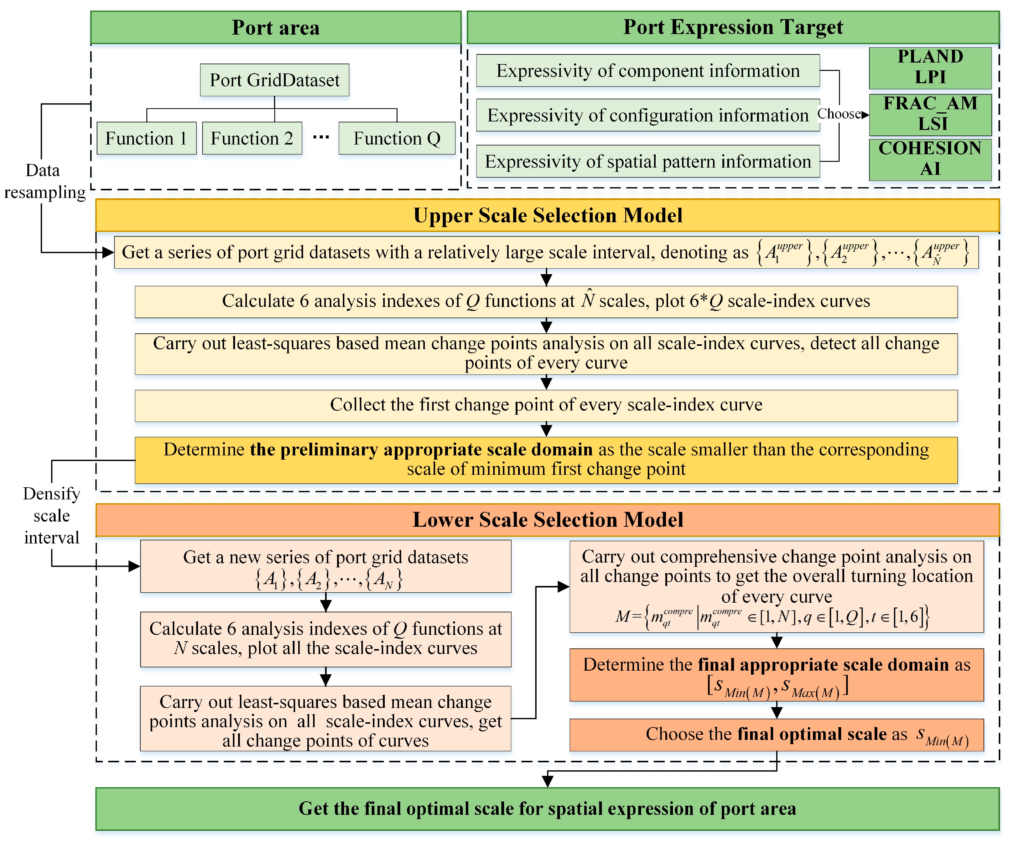
2.1. Two-Layer Scale Selection Framework

The two-layer scale selection framework consists of two parts: a preliminary selection of an appropriate scale domain by the upper layer and a final selection of an optimal scale by the lower layer. The logic of the framework is shown in Figure 3.

In the upper layer, the spatial datasets of the research area at scales with a relatively large interval are collected, and the chosen analysis indices of the research area are calculated separately at these scales. Next, the scale–index curves are plotted, and the change point analysis method is applied to accurately detect all the change points of every curve. Then, an appropriate preliminary scale domain is determined first.

In the lower layer, the appropriate preliminary scale domain is divided by a smaller scale interval. Again, similar spatial dataset collection and index calculation processes are carried out, and the new scale–index curves are plotted. Next, the change point analysis is applied again to obtain all the change points of the curves. Then, a comprehensive change point analysis is carried out on all the change points to obtain the overall turning location of every curve, and the final appropriate scale domain is determined. Finally, the criterion for optimal scale selection is proposed according to the requirement of the research area, and the final optimal scale can then be selected.

In a word, the two layers of the framework separately accomplish a rough search and a precise search of the optimal scale. The upper layer can quickly locate a preliminary appropriate scale domain. The lower layer can further improve the accuracy of scale selection and determine the final appropriate scale domain and the final optimal scale. This paper takes a port area as an example to further clarify the proposed framework.

2.2. Scale Selection Model for Port Spatial Expression

Based on the framework above, a scale selection model for port spatial expression is then established. The whole methodological process of the model is shown in Figure 4. The two-layer scale selection model, which involves the least-squares-based mean change point analysis and the criterion for optimal scale selection, is described in detail as follows.

2.2.1. Data Preprocessing

Referring to the requirements of port spatial expression, the port is classified into Q land use function types, denoted as $\left\{c_q,q=1,2,\dots ,Q\right\}$. Based on the remote-sensing image data, a port grid dataset $\left\{A_1\right\}$ at basic scale $s_1$ is obtained. In the upper scale selection model, the determination of the upper limit scale and the scale interval should consider the extent of the research port area. When the land width of the port area is small, too large a value of the upper limit scale may cause the quantity of the grids for port expression to be too small, and it will not be possible to distinguish the land use functions in a port area well. On the contrary, if the value of the upper limit scale is too small, spatial features at relatively large scales may be neglected, and the subsequent scale selection may be conservative to some extent. Moreover, since some port facilities, such as the roads inside a port area, are located just at the junction of different port functions, the width of roads will then affect the determination of scale interval. Too small a value of the scale interval may result in data redundancy. Conversely, too large a value of the scale interval may influence the identification of land use functions and will thus lead to some port spatial features being missed. Therefore, the upper limit scale and scale interval should be determined according to the real measures of the port. After determining these two parameters, the nearest neighbor algorithm is used to perform data resampling and realize the scaling up of port grid data. A series of port grid datasets $\left\{A_1^{upper}\right\},\left\{A_2^{upper}\right\},\cdots ,\left\{A_{\hat{N}}^{upper}\right\}$, which, respectively, correspond to the incremental scales $\left\{s_n^{upper},n=1,2,\dots ,\hat{N}\right\}$, are obtained. For the lower scale selection model, the scale interval is densified based on the appropriate scale domain preliminarily determined by the upper scale selection model, and port grid datasets $\left\{A_1\right\},\left\{A_2\right\},\cdots ,\left\{A_N\right\}$ are obtained, which, respectively, correspond to the incremental scales $\left\{s_n,n=1,2,\dots ,N\right\}$.

2.2.2. Scale Selection Analysis Index

The variation tendencies of the spatial features of all land use function types are key bases for the selection of optimal scale. Under the guideline of research targets, referring to the landscape metrics chosen in related research works [8,54] and considering the practical spatial features of port land use, a total of 6 landscape metrics on the class level are chosen as representative indices to comprehensively analyze the variations in spatial features in a port area, denoted as $\left\{I_c,c=1,2,\dots ,6\right\}$ (as shown in

Table 1. Description of scale selection analysis indices.

Landscape Metric	Abbreviation	Description	Equation
Percentage of landscape (%)	PLAND	Quantifies the proportional abundance of a given patch type, used here to reflect the expressivity of component information.	$PLAND={\displaystyle \frac{{\displaystyle \sum _{j=1}^{n_p^i}{a}_{ij}}}{A}}\left(100\right)$ $a_{ij}$—area (m2) of patch ij $n_p^i$—number of patches in the landscape of patch type i A—total landscape area (m2)
Largest patch index (%)	LPI	Quantifies the proportion of the largest patch of a given patch type in the total area of the landscape, used here to reflect the expressivity of component information.	$LPI={\displaystyle \frac{\underset{j=1}{\overset{n_p^i}{\max }}\left(a_{ij}\right)}{A}}(100)$
Area-weighted mean fractal dimension index	FRAC_AM	Measures the shape complexity of patches, used here to reflect the expressivity of configuration information.	$FRAC\_AM={\displaystyle \frac{{\displaystyle \sum _{j=1}^{n_p^i}\frac{2\ln \left(0.25p_{ij}\right)}{\ln a_{ij}}\cdot a_{ij}}}{A}}$ $p_{ij}$—perimeter (m) of patch ij
Landscape shape index	LSI	A modified perimeter–area ratio, a measure of overall shape complexity of patches of a given type, used here to reflect the expressivity of configuration information.	$LSI={\displaystyle \frac{0.25{\displaystyle \sum _{i^{\prime }=1}^{n_c}{e}_{i{i}^{\prime }}^{*}}}{\sqrt{A}}}$ $e_{i{i}^{\prime }}^{*}$—total length (m) of the edge in the landscape between patch types i and $i^{\prime }$ $n_c$—number of patch types present in the landscape
Patch cohesion index (%)	COHESION	Measures the physical connectedness of a given patch type, which is better when the index value is smaller. Used here to reflect the expressivity of spatial distribution information.	$COHESION=\left[1-{\displaystyle \frac{{\displaystyle \sum _{j=1}^{n_p^i}{p}_{ij}^{*}}}{{\displaystyle \sum _{j=1}^{n_p^i}{p}_{ij}^{*}\sqrt{a_{ij}^{*}}}}}\right]\cdot {\left[1-{\displaystyle \frac{1}{\sqrt{Z}}}\right]}^{-1}\cdot \left(100\right)$ $p_{ij}^{*}$—perimeter of patch ij in terms of the number of cell surfaces $a_{ij}^{*}$—area of patch ij in terms of the number of cells Z—total number of cells in the landscape
Aggregation index (%)	AI	Measures the level of clumpiness of a given patch type, which is lower when the index value is smaller. Used here to reflect the expressivity of spatial distribution information.	$AI=\left[{\displaystyle \frac{g_{ii}}{\max \to g_{ii}}}\right]\left(100\right)$ $g_{ii}$—number of like adjacencies between pixels of patch type i based on the single-count method

). PLAND and LPI are the indices introduced to evaluate the expressivity of component information, which represents the degree of retention of original component information. FRAC_AM and LSI are the indices introduced to evaluate the expressivity of configuration information, which represents the degree of retention of original configuration information. COHESION and AI are the indices introduced to evaluate the expressivity of spatial distribution information, which represents the degree of retention of original spatial distribution information. A scale performs better when the dataset at this scale can better express these three kinds of information.

2.2.3. Upper Scale Selection Model

Based on the port grid datasets $\left\{A_1^{upper}\right\},\left\{A_2^{upper}\right\},\cdots ,\left\{A_{\hat{N}}^{upper}\right\}$, a total of 6 analysis indices of Q land use function types at $\hat{N}$ scales are calculated. Then, the scale–index curves of all land use function types, which reflect the variation tendencies of indices with the increase in scales, are plotted. In order to analyze the variation characteristics of the curves more accurately, the least-squares-based mean change point analysis is applied to quantitatively detect the change points of scale–index curves. For land use pattern in a port area, the spatial characteristics displayed under a relatively small scale can be more consistent with the actual situation of the port. Therefore, the upper scale selection model collects the first change point of every scale–index curve and sets the scale smaller than the corresponding scale of a minimum first change point as the preliminarily determined appropriate scale domain, which is the basis for optimal scale selection in the lower scale selection model.

2.2.4. Lower Scale Selection Model

Based on the appropriate scale domain determined above, a new series of port grid datasets $\left\{A_1\right\},\left\{A_2\right\},\cdots ,\left\{A_N\right\}$ are obtained by densifying the scale interval. The 6 analysis indices of Q land use types at N scales are calculated, and the corresponding scale–index curves are all plotted. Then, the least-squares-based mean change point analysis is used again to quantitively find out all the change points of scale–index curves. Then, considering the characteristics of every change point of a scale–index curve, a new concept of comprehensive change point is proposed to represent the overall turning point of a curve. The domain between the corresponding scale of the minimum comprehensive change point and maximum comprehensive change point is determined as the final appropriate domain, and the corresponding scale of the minimum comprehensive change point is finally chosen as the optimal scale for port spatial expression.

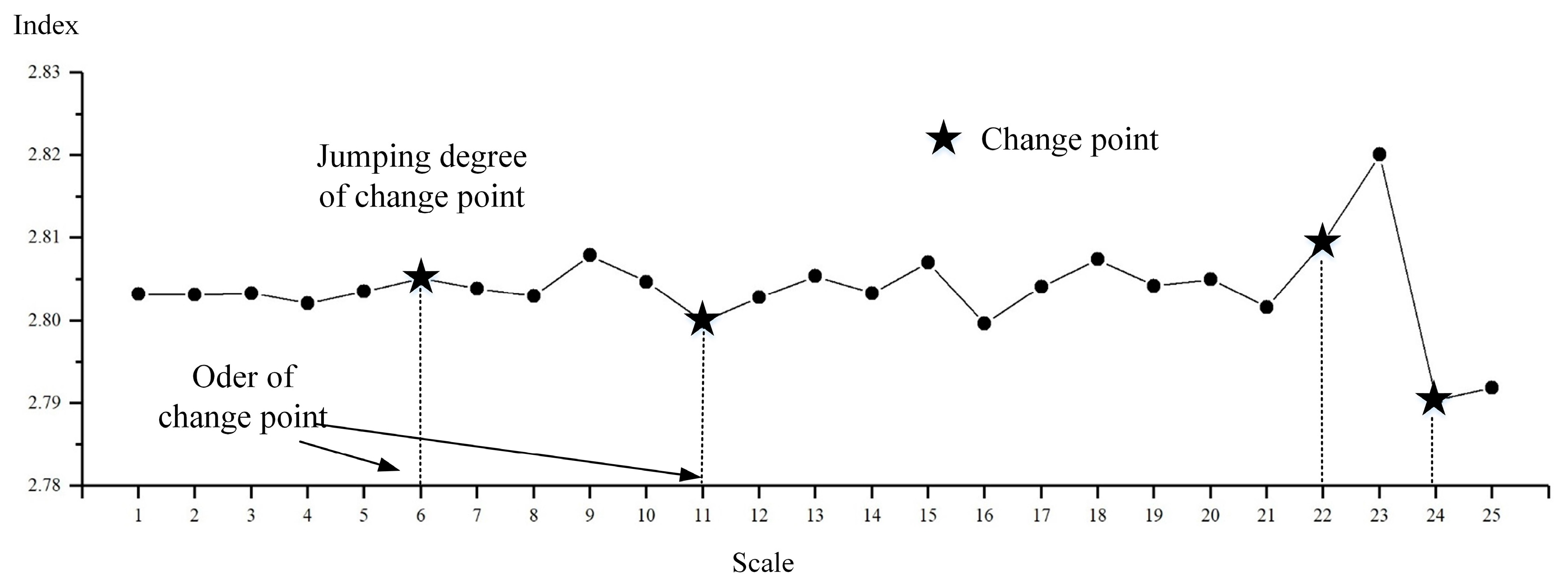
2.2.5. Least-Squares-Based Mean Change Point Analysis

The least-squares-based mean change point analysis method is used in both layers to analyze the variation tendencies of scale–index curves more comprehensively and objectively. Here, the data series $\left\{x_{qt}^n,n=1,2,\dots ,N\right\}\left(q\in \left[1,Q\right],t\in \left[1,6\right]\right)$, which includes the tth index values of the qth land use function type under N scales, is taken as an example to illustrate the process of change point analysis.

The abrupt change in the index values, which occurs at a certain scale location in the data series $\left\{x_{qt}^n,n=1,2,\dots ,N\right\}$, is called a change point. Let

$$\begin{array}{c}{x}_{qt}^n=a_{qt}^n+e_{qt}^n,n=1,2,\dots ,N\\ a_{qt}^1=\dots =a_{qt}^{m_{qt}^1-1}=b_{qt}^1,a_{qt}^{m_{qt}^1}=\dots =a_{qt}^{m_{qt}^2-1}=b_{qt}^2,\dots ,a_{qt}^{m_{qt}^K}=\dots =a_{qt}^N=b_{qt}^{K+1}\end{array}\}$$

(1)

where $1<m_{qt}^1<m_{qt}^2<\dots <m_{qt}^k<\dots <m_{qt}^K\le N$, $e_{qt}^n$ is the random error term, whose variance is ${\sigma }^2$, and the expected value is 0; K is the number of change points; $m_{qt}^k$ is the kth change point location.

Null hypothesis H: There is no change point, which means $b_{qt}^1=\dots =b_{qt}^{K+1}$.

When $S-S^{*}>C_{\alpha }$, null hypothesis H is negated; namely, there exist change points.

$$\begin{array}{c}S={{\displaystyle \sum _{n=1}^N\left(x_{qt}^n-\overline{X}\right)}}^2\\ \overline{X}={\displaystyle \frac{{\displaystyle \sum _{n=1}^N{x}_{qt}^n}}{N}}\end{array}\}$$

(2)

$$\begin{array}{c}{S}^{*}=\min \left(S_2,S_3,\dots ,S_{n_1}\right)\\ S_{n_1}={{\displaystyle \sum _{n_2=1}^{n_1-1}\left(x_{qt}^{n_2}-{\overline{X}}_{n_1^1}\right)}}^2+{{\displaystyle \sum _{n_2=n_1}^N\left(x_{qt}^{n_2}-{\overline{X}}_{n_1^2}\right)}}^2\left(2\le n_1\le N\right)\end{array}\}$$

(3)

where ${\overline{X}}_{n_1^1}$ and ${\overline{X}}_{n_1^2}$ are separately the arithmetic mean values of two subseries $x_{qt}^1,x_{qt}^2,\mathrm{\dots },x_{qt}^{n_1-1}$ and $x_{qt}^{n_1},x_{qt}^{n_1+1},\dots ,x_{qt}^N$, which are segmented by $n_1$.

Calculate the value of $C_{\alpha }$ under significant level $\alpha$.

$$C_{\alpha }={\sigma }^2\left\{2\log \log N+\log \log \log N-\log \pi -2\log \left[-0.5\log \left(1-\alpha \right)\right]\right\}$$

(4)

where ${\sigma }^2$ is usually unknown and can be estimated by Equation (5).

$${\sigma }^2={\displaystyle \frac{S^{*}}{N-2\log \log N-\log \log \log N-2.4}}$$

(5)

Then, the least-squares method is used to find out the change points of the data series. The locations of all the change points are estimated by minimizing the target function T in Equation (6), where $m_{qt}^0=1,\begin{array}{l}\hfill \end{array}{m}_{qt}^{K+1}=N+1$.

$$\mathrm{T}=\mathrm{T}\left(m_{qt}^1,\dots ,m_{qt}^K,b_{qt}^1,\dots ,b_{qt}^{K+1}\right)={{\displaystyle \sum _{k=1}^{K+1}{\displaystyle \sum _{n=m_{qt}^{k-1}}^{m_{qt}^k-1}\left(x_{qt}^n-b_{qt}^k\right)}}}^2$$

(6)

The above optimization problem can be further simplified by minimizing Equation (7).

$$\begin{array}{c}\mathrm{T}=\mathrm{T}\left(m_{qt}^1,\dots ,m_{qt}^K\right)={{\displaystyle \sum _{k=1}^{K+1}{\displaystyle \sum _{n=m_{qt}^{k-1}}^{m_{qt}^k-1}\left(x_{qt}^n-y_{qt}^k\right)}}}^2\\ y_{qt}^k={\displaystyle \frac{\left(x_{qt}^{m_{qt}^{k-1}}+\dots +x_{qt}^{m_{qt}^k-1}\right)}{m_{qt}^k-m_{qt}^{k-1}}}\end{array}\}$$

(7)

where $y_{qt}^k$ is the arithmetic mean value of subseries $\left\{x_{qt}^n,n\in \left[m_{qt}^{k-1},m_{qt}^k-1\right]\right\}$. Based on the change point estimation results when K = 1, step-by-step adjustment is carried out within the range $1<m_{qt}^1<m_{qt}^2<\dots <m_{qt}^k<\dots <m_{qt}^K\le N$ to realize the minimization of function T when K > 1. The change point locations for the tth index of the qth land use function type can then be obtained, denoted as $\left\{m_{qt}^k|m_{qt}^k\in [1,N],k\in [1,K]\right\}$.

2.2.6. Comprehensive Change Point Analysis and Criterion for Optimal Scale Selection in a Port Area

Based on the change point locations already determined via mathematical statistical analysis in the lower scale selection model, how to select the final optimal scale becomes a key problem. As shown in Figure 4, comprehensive change point analysis is then carried out based on the obtained change points to obtain the overall turning location of every curve, and the final optimal scale can then be determined by the criterion based on the comprehensive change point analysis results. The criterion for optimal scale selection is set according to the requirement of the research. The detailed description of the proposed comprehensive change point analysis method is as follows.

As shown in Figure 5, for the change point locations determined in the lower scale selection model, there exists a phenomenon whereby the variation extent of a change point in a front location may not be the most distinct, while a change point with more prominent variation may be located in the rear. That is to say, the variation extent of the first change point location, which is detected by the mean change point analysis, may not be the most obvious, and if all the first change points are chosen to determine the final appropriate scale, the value of the final selected scale may be a little conservative. Although the accuracy of expression is ensured, the connection between the port area and the surrounding city and sea area may face inconvenience. Therefore, the change points which will be chosen to determine the final appropriate scale need to be adjusted to balance the requirements of spatial expression accuracy and connection convenience.

Therefore, a compromise is made between the order of change point locations and the variation extent of change points, and a new concept of a comprehensive change point is proposed. It is defined as the comprehensive change point location of a scale–index curve, which represents the overall turning location of the curve from a mathematical perspective. The comprehensive change point is calculated as the weighted sum of all change point locations of the curve. The determination of the weight considers both the order of change point locations and the variation extent of change points, which is measured by the jumping degrees of change points in this paper. The specific calculation process is as follows.

Step 1: First, for the change point set $\left\{m_{qt}^k|m_{qt}^k\in [1,N],k\in [1,K]\right\}$, record the order of every change point location, namely k, and calculate its corresponding jumping degree, denoted as ${\theta }_k\left(k=1,2,\dots ,K\right)$.

Step 2: Next, construct the order weight ${\omega }_{1k}=F(k)$ to represent the influence of the order of change point locations, and obtain the order weight set $\left\{{\omega }_{1k}\right\}$ by calculating the order weight of every change point.

Step 3: Then, based on the order weight above, further considering the influence of the variation extent of change points, construct the comprehensive weight ${\omega }_{2k}=G({\omega }_{1k},{\theta }_k)$, which is composed of the jumping degree and the order weight, and obtain the comprehensive weight set $\left\{{\omega }_{2k}\right\}$ by calculating the comprehensive weight of every change point. Functions F and G need to be built according to the practical characteristics of the scale–index curves of a port. In the case study in this paper, considering the variation characteristics of the scale–index curves in the research port area, functions F and G are established as follows.

$${\omega }_{1k}=F(k)={\displaystyle \frac{K-k+1}{\left(K+1\right)K/2}},\begin{array}{l}\hfill \end{array}\begin{array}{l}k\in [1,K]\hfill \end{array}$$

(8)

$$\begin{array}{c}{\omega }_{2k}=G({\omega }_{1k},{\theta }_k)={\displaystyle \frac{{\omega }_{1k}{\theta }_k}{{\displaystyle \sum _{k=1}^K{\omega }_{1k}{\theta }_k}}},\begin{array}{l}\hfill \end{array}\begin{array}{l}k\in [1,K]\hfill \end{array}\\ {\theta }_k={\displaystyle \sum _{n=m_{qt}^k}^{m_{qt}^{k+1}-1}{x}_{qt}^n/\left(m_{qt}^{k+1}-m_{qt}^k\right)}-{\displaystyle \sum _{n=m_{qt}^{k-1}}^{m_{qt}^k-1}{x}_{qt}^n/\left(m_{qt}^k-m_{qt}^{k-1}\right)},\begin{array}{l}\hfill \end{array}\begin{array}{l}k\in [1,K]\hfill \end{array}\end{array}\}$$

(9)

Step 4: Then, the comprehensive weighted calculation of all change points is carried out according to Equation (10), and the comprehensive change point of the tth index of the qth land use function type is obtained, namely $m_{qt}^{compre}$. With this method, the comprehensive change points of all scale–index curves are calculated, and the comprehensive change point set is obtained, denoted as $M=\left\{m_{qt}^{compre}|m_{qt}^{compre}\in [1,N],q\in \left[1,Q\right],t\in \left[1,6\right]\right\}$.

$$m_{qt}^{compre}={\displaystyle \sum _{k=1}^K{\omega }_{2k}{m}_{qt}^k}$$

(10)

The final appropriate scale domain in the lower model can be denoted as $[s_{Min\left(M\right)},s_{Max\left(M\right)}]$. In order to guarantee the expressivities of the component information, configuration information and spatial pattern information of all land use function types, the criterion for optimal scale selection in a port area is set as the corresponding scale of the minimum comprehensive change point. The final optimal scale for port spatial expression is denoted as $s_{Min\left(M\right)}$.

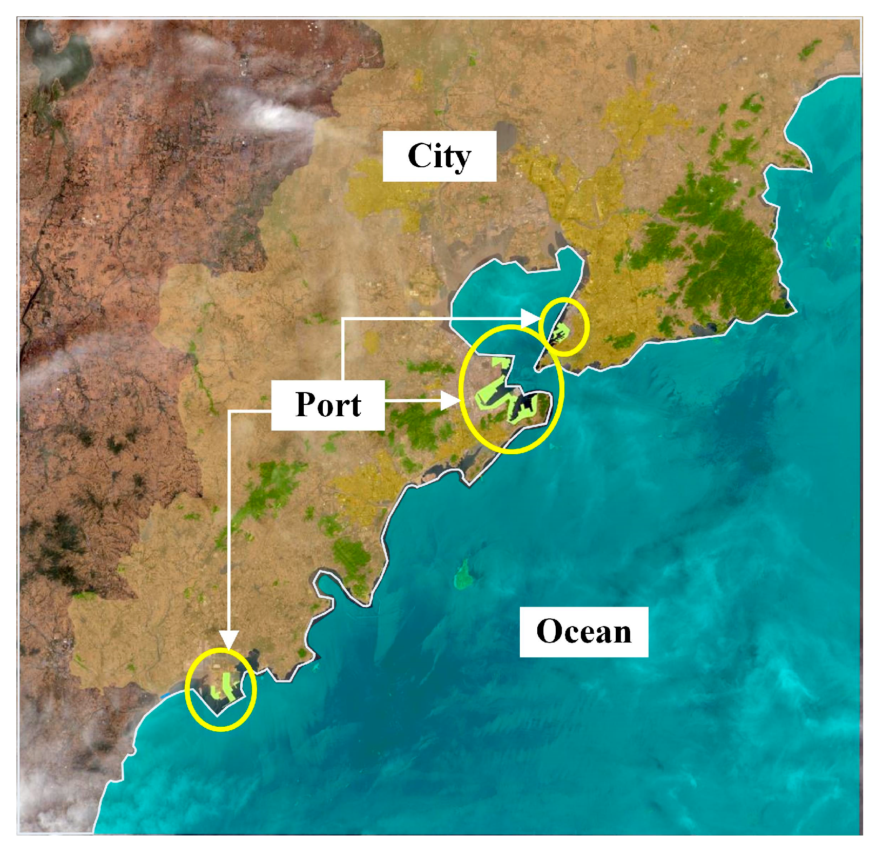
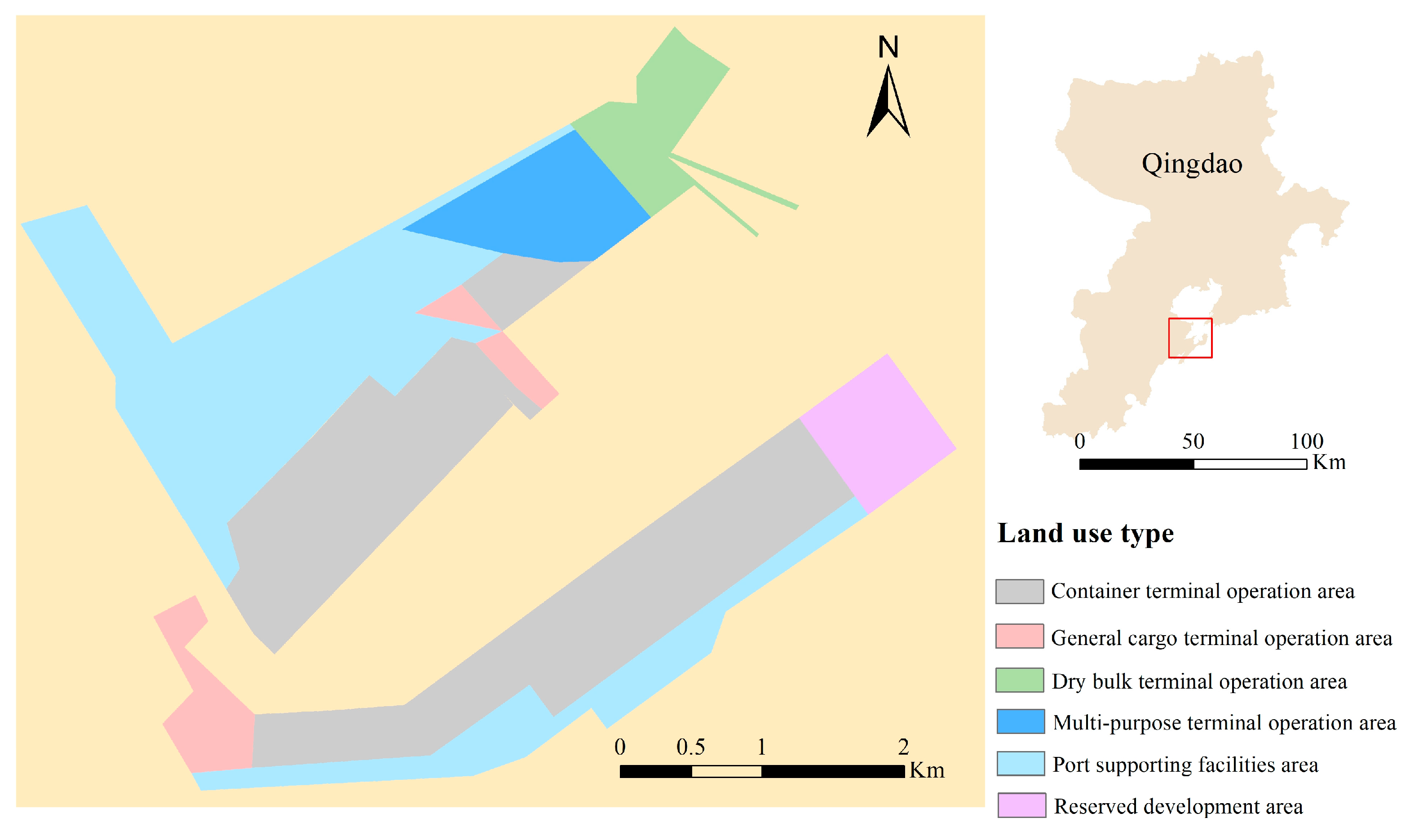
2.3. Research Area and Data

Qingdao is an important port city located in eastern China, and the port throughput in Qingdao is in the front rank of the world. This paper takes a port area in Qingdao as an example to verify the feasibility of the proposed scale selection model for port spatial expression and determine a suggested optimal scale.

Since the extent of the research port area is small, and the distribution of land use functions in the port area is relatively orderly, high-resolution Google Earth images from 2020, which possess a spatial resolution of over 2 m, were utilized in this paper. The land use functions were identified based on the high-resolution Google Earth images, and previous port planning information on the research port area was also applied here to improve the accuracy of classification.

Referring to the port functions in a port area [53], a total of 6 kinds of land use types were visually mapped (as shown in

Table 2. Description of land use function types in a port area.

Land Use Function Types in a Port Area	Description
Container terminal operation area	Land use for production and operation of container terminals
General cargo terminal operation area	Land use for production and operation of general cargo terminals
Dry bulk terminal operation area	Land use for production and operation of dry bulk terminals
Multi-purpose terminal operation area	Land use for production and operation of multi-purpose terminals
Port supporting facilities area	Land use for other port facilities, which support the daily operation of the port
Reserved development area	Land use reserved for future port development

), and a port grid dataset under spatial scale 2 m was produced as the basic grid dataset (as shown in Figure 6).

Since the smallest land width in this port area is measured to be about 400 m, and the roads inside this port area are measured to be about 7~15 m, repeated attempts were carried out to determine the value of the upper limit scale and scale interval. And it was finally found that the quantity of grids is relatively reasonable, and the expression of land use functions is basically complete when the upper limit scale is set at 200 m, and the scale interval is set at 10 m. Then, data resampling via the nearest neighbor algorithm was carried out using ArcGIS 10.6, and 20 port grid datasets, corresponding to scales from 10 m to 200 m, were then obtained as the data foundation of the upper scale selection model. The analysis indices used for scale selection were calculated using the software Fragstats 4.2 [55], and the mathematical analysis of the scale–index curves was conducted based on Python 3.7.

3. Results

3.1. Analysis of Scale–Index Curves in the Upper Scale Selection Model

Based on the 20 port grid datasets, a total of 6 analysis indices of 6 land use function types under 20 scales were calculated, and 36 scale–index curves were plotted (as shown in Figure 7). Least-squares-based mean change point analysis was carried out for these 36 curves, and the detected change points are listed in

Table 3. Results of change point analysis for PLAND, LPI, FRAC_AM, LSI, COHESION and AI.

Analysis Index	Land Use Function In the Port Area	Change Point	Corresponding Scale of Change Point (m)
PLAND	Container terminal operation area	5, 8, 9, 12, 15	50, 80, 90, 120, 150
	General cargo terminal operation area	6, 11, 14	60, 110, 140
	Dry bulk terminal operation area	5, 12, 14, 15	50, 120, 140, 150
	Multi-purpose terminal operation area	6, 9, 11, 13, 15	60, 90, 110, 130, 150
	Port supporting facilities area	6, 12, 14	60, 120, 140
	Reserved development area	6, 7, 11, 13, 16	60, 70, 110, 130, 160
LPI	Container terminal operation area	6, 8, 9, 14, 18	60, 80, 90, 140, 180
	General cargo terminal operation area	5, 6, 11, 13, 16	50, 60, 110, 130, 160
	Dry bulk terminal operation area	5, 8, 12, 13, 18	50, 80, 120, 130, 180
	Multi-purpose terminal operation area	6, 9, 11, 13, 15	60, 90, 110, 130, 150
	Port supporting facilities area	9, 12	90, 120
	Reserved development area	11, 16	110, 160
FRAC_AM	Container terminal operation area	5, 6, 12, 14, 16	50, 60, 120, 140, 160
	General cargo terminal operation area	5, 10, 12, 17	50, 100, 120, 170
	Dry bulk terminal operation area	5, 7, 10, 13, 18	50, 70, 100, 130, 180
	Multi-purpose terminal operation area	6, 11, 14, 17	60, 110, 140, 170
	Port supporting facilities area	6, 9, 12, 18	60, 90, 120, 180
	Reserved development area	6, 8, 10, 13, 18	60, 80, 100, 130, 180
LSI	Container terminal operation area	5, 10, 12, 18	50, 100, 120, 180
	General cargo terminal operation area	7, 10, 15, 19	70, 100, 150, 190
	Dry bulk terminal operation area	6, 7, 14, 17	60, 70, 140, 170
	Multi-purpose terminal operation area	6, 9, 14, 16	60, 90, 140, 160
	Port supporting facilities area	5, 8, 12, 15, 18	50, 80, 120, 150, 180
	Reserved development area	6, 8, 14, 18	60, 80, 140, 180
COHESION	Container terminal operation area	5, 9, 13, 17	50, 90, 130, 170
	General cargo terminal operation area	5, 9, 13, 17	50, 90, 130, 170
	Dry bulk terminal operation area	5, 10, 13, 20	50, 100, 130, 200
	Multi-purpose terminal operation area	5, 9, 13, 17	50, 90, 130, 170
	Port supporting facilities area	5, 9, 13, 18	50, 90, 130, 180
	Reserved development area	5, 9, 13, 17	50, 90, 130, 170
AI	Container terminal operation area	5, 9, 13, 16	50, 90, 130, 160
	General cargo terminal operation area	5, 9, 13, 16	50, 90, 130, 160
	Dry bulk terminal operation area	5, 8, 9, 11, 18	50, 80, 90, 110, 180
	Multi-purpose terminal operation area	5, 9, 12, 16	50, 90, 120, 160
	Port supporting facilities area	5, 9, 13, 17	50, 90, 130, 170
	Reserved development area	5, 11, 15, 18	50, 110, 150, 180

. The change point locations 1~20, respectively, correspond to scales 10~200 m.

In Figure 7 and Table 3, it can be found that the scale–index curves of PLAND and LPI show a stable tendency in the early stage and represent unstable fluctuations in the later stage, while the curves of the other four indices all show an overall downward tendency. Among the other four indices, the fluctuations of FRAC_AM and LSI with the increase in scale are more intense compared with those of COHESION and AI. The curves of COHESION and AI both decline at a relatively stable speed as the scale increases.

Since there exists a trestle wharf, which is a narrow and long space extending to the water area in the dry bulk terminal operation area, the variations in indices in the dry bulk terminal operation area are all more sensitive to the increase in scales, especially FRAC_AM and LSI, which represent the expressivity of configuration information. The variations in FRAC_AM and LSI in the dry bulk terminal operation area both suffer obvious decline, respectively, around the scale of 50 m and 60 m, which means that the configuration of the dry bulk terminal operation area is complex and gradually becomes regular when the scale increases. The curves of PLAND and LPI of the dry bulk terminal operation area fluctuate sharply beyond the scale of 50 m, which means that the component information of the dry bulk terminal operation area is relatively accurate within the scale of 50 m. The variations in COHESION and AI first decline smoothly but begin to change the tendency, respectively, from the scale of 50 m, which reflects that the physical connectedness and aggregation degree of the dry bulk terminal operation area both decrease when the scale increases, and the decrease process is not stable.

As shown in Table 3, for all land use function types, the corresponding scales of the calculated first change points include 50 m, 60 m, 70 m, 90 m and 110 m, where 50 m is the minimum and occupies the majority. Moreover, in Figure 7, it can also be found that the variations in all indices are mainly stable within the scale of 50 m, which means that the expressivities of component information, configuration information and spatial distribution information are closer to the real features of the port when the scale is within 50 m. Therefore, the scale domain [2 m, 50 m] is chosen as the preliminarily determined appropriate scale domain to help carry out further a more precise scale selection process.

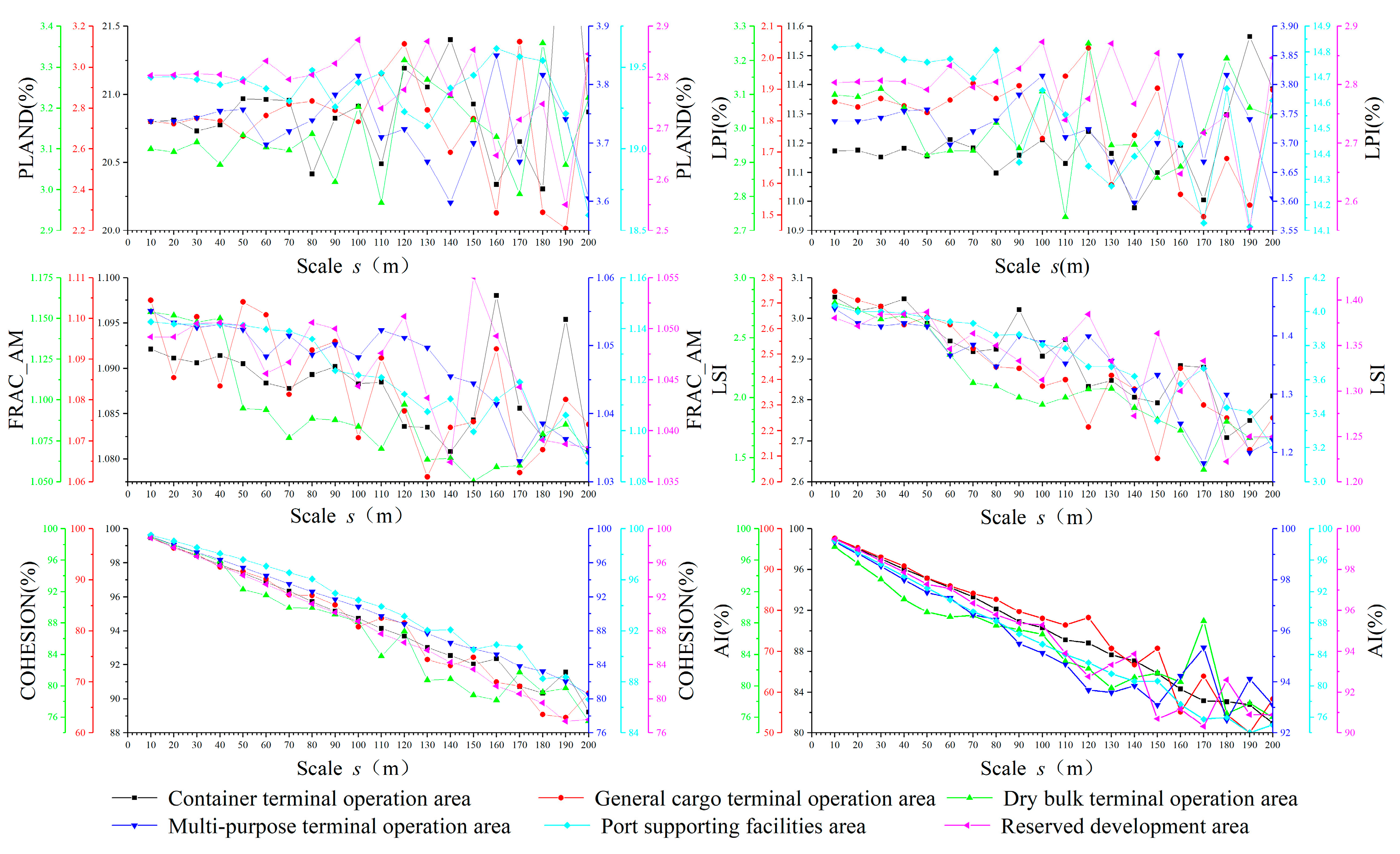
3.2. Analysis of Scale–Index Curves in the Lower Scale Selection Model

As can be seen in Figure 6, there exists a localized narrow space in the container terminal operation area, and the scope of the general cargo terminal operation area is relatively small and scattered. Moreover, there is a narrow and long trestle wharf in the dry bulk terminal operation area. Therefore, the requirement for the accuracy of port spatial expression becomes higher. Therefore, the preliminarily determined appropriate scale domain [2 m, 50 m] was densified by a scale interval of 2 m, and a series of new port grid datasets under 25 scales were obtained.

Since the curves of COHESION and AI in this case both basically show a uniform linear decrease within the scale of 50 m, the variations in the other four indices are focused on as the basis for the lower scale selection process. These 4 analysis indices of 6 land use function types under 25 scales were calculated, and 24 new scale–index curves were plotted (as shown in Figure 8). It can be found that the four indices show different degrees of fluctuations with the increase in scale. The fluctuations of PLAND and LPI are both small in the early stage while large in the later stage, which indicates that the expressivity of component information of all land use function types is more accurate when the scale is relatively small. The fluctuations of FRAC_AM and LSI show a gradual decline tendency as the scale increases, indicating that the complexity of the configuration information of all land use function types decreases overall as the scale increases. For the dry bulk terminal operation area in particular, its FRAC_AM index shows a prominent decrease beyond the scale of 40 m, which is consistent with the calculation result of this curve’s comprehensive change point.

3.3. Comprehensive Change Point Analysis and Optimal Scale Selection

The least-squares-based mean change point analysis was performed on all the scale–index curves in the lower scale selection model, and the calculated change point locations are listed in

Table 4. Results of change point analysis and calculation of comprehensive change points for PLAND, LPI, FRAC_AM and LSI.

Analysis Index	Land Use Function in the Port Area	Change Point	Corresponding Scale of Change Point (m)	Comprehensive Change Point	Corresponding Scale of Comprehensive Change Point (m)
PLAND	Container terminal operation area	5, 15, 18	10, 30, 36	16	32
	General cargo terminal operation area	11, 14, 15, 22	22, 28, 30, 44	14	28
	Dry bulk terminal operation area	9, 14, 16	18, 28, 32	16	32
	Multi-purpose terminal operation area	8, 16, 18	16, 32, 36	16	32
	Port supporting facilities area	5, 11, 18	10, 22, 36	14	28
	Reserved development area	6, 11, 22, 24	12, 22, 44, 48	20	40
LPI	Container terminal operation area	11, 18, 19	22, 36, 38	18	36
	General cargo terminal operation area	10, 15	20, 30	12	24
	Dry bulk terminal operation area	9, 14, 16, 23	18, 28, 32, 46	20	40
	Multi-purpose terminal operation area	8, 16, 18	16, 32, 36	16	32
	Port supporting facilities area	7, 10, 17, 18, 22	14, 20, 34, 36, 44	16	32
	Reserved development area	5, 9, 10, 13, 23, 24	10, 18, 20, 26, 46, 48	17	34
FRAC_AM	Container terminal operation area	3, 5, 7, 13, 15, 18	6, 10, 14, 26, 30, 36	7	14
	General cargo terminal operation area	3, 7, 8, 10, 13, 19	6, 14, 16, 20, 26, 38	9	18
	Dry bulk terminal operation area	7, 10, 14, 22, 23	14, 20, 28, 44, 46	20	40
	Multi-purpose terminal operation area	3, 6, 9, 13, 14, 22	6, 12, 18, 26, 28, 44	11	22
	Port supporting facilities area	4, 8, 10, 13, 19, 22	8, 16, 20, 26, 38, 44	11	22
	Reserved development area	10, 12, 13, 20, 21	10, 24, 26, 40, 42	14	28
LSI	Container terminal operation area	4, 10, 12, 16, 21	8, 20, 24, 32, 42	9	18
	General cargo terminal operation area	4, 7, 9, 12, 15, 19	8, 14, 18, 24, 30, 38	10	20
	Dry bulk terminal operation area	4, 10, 14, 20, 23	8, 20, 28, 40, 46	12	24
	Multi-purpose terminal operation area	5, 9, 15, 16, 22	10, 18, 30, 32, 44	11	22
	Port supporting facilities area	5, 8, 10, 13, 14, 21, 22	10, 16, 20, 26, 28, 42, 44	12	24
	Reserved development area	5, 10, 13, 21	10, 20, 26, 42	10	20
COHESION	Container terminal operation area	5, 15, 18	10, 30, 36	16	32
	General cargo terminal operation area	11, 14, 15, 22	22, 28, 30, 44	14	28
	Dry bulk terminal operation area	9, 14, 16	18, 28, 32	16	32
	Multi-purpose terminal operation area	8, 16, 18	16, 32, 36	16	32
	Port supporting facilities area	5, 11, 18	10, 22, 36	14	28
	Reserved development area	6, 11, 22, 24	12, 22, 44, 48	20	40
AI	Container terminal operation area	11, 18, 19	22, 36, 38	18	36
	General cargo terminal operation area	10, 15	20, 30	12	24
	Dry bulk terminal operation area	9, 14, 16, 23	18, 28, 32, 46	20	40
	Multi-purpose terminal operation area	8, 16, 18	16, 32, 36	16	32
	Port supporting facilities area	7, 10, 17, 18, 22	14, 20, 34, 36, 44	16	32
	Reserved development area	5, 9, 10, 13, 23, 24	10, 18, 20, 26, 46, 48	17	34

. The change point locations 1~25, respectively, correspond to scales 2~50 m.

According to the variation characteristics of indices, which represent the spatial features of the port area, functions F and G were built via Equations (8) and (9), and the comprehensive change points for 24 scale–index curves were calculated and are listed in Table 4. As can be seen, the locations of comprehensive change points are distributed between 7 and 20, corresponding to the scale domain ranging from 14 m to 40 m. The comprehensive change point of every scale–index curve represents the overall turning point of the curve from a mathematical perspective.

Taking the dry bulk terminal operation area as an example, it can be found that the fluctuation of the scale–PLAND curve increases rapidly beyond the scale of 32 m, while the downward trend of the scale–LSI curve begins to suffer an obvious fluctuation beyond the scale of 24 m. Moreover, it is obvious that the scale–LPI curve and the scale–FRAC_AM curve both appear to experience a prominent decline beyond the scale of 40 m. That is to say, the proposed comprehensive change point analysis can well reflect the overall turning locations of the four curves of the dry bulk terminal operation area.

Therefore, the finally determined appropriate scale domain is [14 m, 40 m]. Within this scale domain, the variations in the four indices are all relatively steady, which means that the expressivities of component information, configuration information and spatial distribution information of all land use function types are more accurate and can better reflect the reality of the port area. And the corresponding scale of the minimum comprehensive change point of 14 m is suggested to be the final optimal scale for the spatial expression of the research port area.

4. Discussion

This paper proposes a universal quantitative two-layer framework, which is applicable to different sizes of research areas, in order to help improve the efficiency and precision of spatial scale selection. Spatial scale selection in a port area is one application of the proposed framework in a relatively small research area.

Different from previous studies, which analyzed the scale effect of a large number of landscape indices [2,12], the analysis indices chosen in this paper are goal-oriented. The expressivities of component information, configuration information and spatial distribution information of all land use functions are the three main targets that the framework focuses on, and six representative indices at the class level are selected accordingly. By analyzing the landscape metrics at different scales, it is noted that, in agreement with previous research studies [42,56], different landscape metrics of different land use functions possess different degrees of scale dependence. This further reflects that the expressivities of component information, configuration information and spatial distribution information are influenced by spatial scale to a different degree. And the expressivity of configuration information is relatively more sensitive to a change in scale.

In the case study of port scale selection, the optimal spatial scale for port expression is suggested to be 14 m. Compared with the optimal scale determined in scale-related studies (e.g., 30–60 m [56], 50 m [12], 150 m [18]), the scale selected in this paper seems to be relatively small. This is because the extent of the research port area is relatively small, and the requirement for accuracy of spatial expression in a port area is relatively high. In Figure 8, it can be found that the determined optimal scale of 14 m can well satisfy the requirements of the expressivities.

The proposed two-layer framework realizes the scale selection process by a rough search in the upper layer and a precise search in the lower layer. This design can quickly locate an appropriate scale domain and further precisely find out the optimal scale. Moreover, a least-squares-based mean change point analysis method is introduced into the framework to quantitatively detect all the change points of the scale–index curve, since the variation in the scale–index curve may sometimes be difficult and inaccurate, to find out the turning locations just by visual observation. And in Table 3 and Figure 7, it can be proved that the calculated change points can indeed reflect the variation tendencies of scale–index curves. Moreover, a new concept of a comprehensive change point, which represents the overall turning location of the curve, is also proposed and introduced into the framework, so as to balance the requirements of improving data accuracy and reducing data redundancy. As can be found in Table 4 and Figure 8, the comprehensive change point analysis results can well reflect the overall turning tendency of a curve. Compared with previous studies, where the optimal spatial scales used for expression and analysis were determined with a certain degree of subjectivity [41,42], the above mathematical analysis methods, which are introduced into the framework, can improve the efficiency and precision of spatial scale selection.

Via the framework proposed in this paper, the selection process of an optimal scale for the spatial expression of a research area can be more scientific and systematic. Future work will further improve the analysis indices corresponding to the targets of the framework to reveal the scale effect in different sizes of research areas.

5. Conclusions

The accuracy of spatial expression is closely related to spatial scale, which is defined as the size of the grid in this paper. In order to reasonably determine the optimal scale for spatial expression, this paper proposes a two-layer framework for the scale selection process of all sizes of research areas. A port area is taken as an example to systematically clarify the application of this framework, and a scale selection model for port spatial expression is established. A least-squares-based mean change point analysis method and a new concept of a comprehensive change point are introduced to help determine the final optimal scale. A port area in Qingdao in eastern China is taken as an example to verify the feasibility of the proposed model. The results prove that the proposed scale selection model can well recognize the overall turning location of every scale–index curve, and the optimal scale selected via the proposed framework can satisfy the requirements of the expressivities of component information, configuration information and spatial distribution information. The optimal scale for the research port area is finally suggested to be 14 m.

This paper systematically deals with the spatial scale selection problem. The proposed two-layer framework can improve the efficiency of optimal scale selection, provide the methodological references for planners to better spatialize the research area and lay a solid foundation for subsequent spatial planning work.

References

1. Atkinson, P.M.; Tate, N.J. Spatial scale problems and geostatistical solutions: A review. Prof. Geogr. 2000, 52, 607–623. [Google Scholar] [CrossRef]
2. Wu, J.G.; Shen, W.J.; Sun, W.Z.; Tueller, P.T. Empirical patterns of the effects of changing scale on landscape metrics. Landsc. Ecol. 2002, 17, 761–782. [Google Scholar] [CrossRef]
3. Wu, J.G. Effects of changing scale on landscape pattern analysis: Scaling relations. Landsc. Ecol. 2004, 19, 125–138. [Google Scholar] [CrossRef]
4. Woodcock, C.E.; Strahler, A.H. The factor of scale in remote sensing. Remote Sens. Environ. 1987, 21, 311–332. [Google Scholar] [CrossRef]
5. Dragut, L.; Eisank, C.; Strasser, T. Local variance for multi-scale analysis in geomorphometry. Geomorphology 2011, 130, 162–172. [Google Scholar] [CrossRef]
6. Yang, D.W.; Herath, S.; Musiake, K. Spatial resolution sensitivity of catchment geomorphologic properties and the effect on hydrological simulation. Hydrol. Process. 2001, 15, 2085–2099. [Google Scholar] [CrossRef]
7. Lu, X.Y.; Li, Y.K.; Washington-Allen, R.A.; Li, Y.N.; Li, H.D.; Hu, Q.W. The effect of grid size on the quantification of erosion, deposition, and rill network. Int. Soil Water Conserv. Res. 2017, 5, 241–251. [Google Scholar] [CrossRef]
8. Liu, H.; Weng, Q.H. Scaling effect on the relationship between landscape pattern and land surface temperature: A case study of Indianapolis, United States. Photogramm. Eng. Remote Sens. 2009, 75, 291–304. [Google Scholar] [CrossRef]
9. Wu, Q.; Li, Z.Y.; Yang, C.B.; Li, H.Q.; Gong, L.W.; Guo, F.X. On the scale effect of relationship identification between land surface temperature and 3D landscape pattern: The application of random forest. Remote Sens. 2022, 14, 279. [Google Scholar] [CrossRef]
10. Liu, X.L.; Wang, Y.; Li, Y.; Liu, F.; Shen, J.L.; Wang, J.; Xiao, R.L.; Wu, J.S. Multi-scaled response of groundwater nitrate contamination to integrated anthropogenic activities in a rapidly urbanizing agricultural catchment. Environ. Sci. Pollut. Res. 2019, 26, 34931–34942. [Google Scholar] [CrossRef]
11. Lü, Y.H.; Feng, X.M.; Chen, L.D.; Fu, B.J. Scaling effects of landscape metrics: A comparison of two methods. Phys. Geogr. 2013, 34, 40–49. [Google Scholar] [CrossRef]
12. Tian, P.; Cao, L.D.; Li, J.L.; Pu, R.L.; Shi, X.L.; Wang, L.J.; Liu, R.Q.; Xu, H.; Tong, C.; Zhou, Z.J.; et al. Landscape grain effect in Yancheng Coastal Wetland and its response to landscape changes. Int. J. Environ. Res. Public Health 2019, 16, 2225. [Google Scholar] [CrossRef] [PubMed]
13. Huang, D.; Yang, X.H.; Dong, N.; Cai, H. Evaluating Grid Size Suitability of Population Distribution Data via Improved ALV Method: A Case Study in Anhui Province, China. Sustainability 2017, 10, 41. [Google Scholar] [CrossRef]
14. Chen, S.H.; Zhang, R.H.; Su, H.B.; Tian, J.; Xia, J. Scaling-up transformation of multisensor images with multiple resolutions. Sensors 2009, 9, 1370–1381. [Google Scholar] [CrossRef]
15. Wang, Q.M.; Shi, W.Z.; Atkinson, P.M.; Zhao, Y.L. Downscaling MODIS images with Area-to-Point Regression Kriging. Remote Sens. Environ. 2015, 166, 191–204. [Google Scholar] [CrossRef]
16. Jantz, C.A.; Geotz, S.J. Analysis of scale dependencies in a urban land-use change model. Int. J. Geogr. Inf. Sci. 2005, 19, 217–241. [Google Scholar] [CrossRef]
17. Wolock, D.M.; Price, C.V. Effects of digital elevation model map scale and data resolution on a topography-based watershed model. Water Resour. Res. 1994, 30, 3041–3052. [Google Scholar] [CrossRef]
18. Yaermaimaiti, A.; Li, X.G.; Ge, X.Y.; Liu, C.J. Analysis of landscape pattern and ecological risk change characteristics in Bosten Lake basin based on optimal scale. Ecol. Indic. 2024, 163, 112120. [Google Scholar] [CrossRef]
19. Zhao, Y.; Feng, Q. Identifying spatial and temporal dynamics and driving factors of cultivated land fragmentation in Shaanxi province. Agric. Syst. 2024, 217, 103948. [Google Scholar] [CrossRef]
20. Marceau, D.J.; Gratton, D.J. Remote sensing and the measurement of geographical the entities in a forested environment: 2. The optimal spatial resolution. Remote Sens. Environ. 1994, 49, 105–117. [Google Scholar] [CrossRef]
21. Atkinson, P.M.; Curran, P.J. Choosing an appropriate spatial resolution for remote sensing investigations. Photogramm. Eng. Remote Sens. 1997, 63, 1345–1351. [Google Scholar]
22. Ming, D.P.; Yang, J.Y.; Li, L.X.; Song, Z.Q. Modified ALV for selecting the optimal spatial resolution and its scale effect on image classification accuracy. Math. Comput. Model. 2011, 54, 1061–1068. [Google Scholar] [CrossRef]
23. Li, R.X.; Gao, X.H.; Shi, F.F.; Zhang, H. Scale effect of land cover classification from multi-resolution satellite remote sensing data. Sensors 2023, 23, 6136. [Google Scholar] [CrossRef] [PubMed]
24. Guo, L.; Liu, R.; Men, C.; Wang, Q.; Miao, Y.; Shoaib, M.; Wang, Y.; Jiao, L.; Zhang, Y. Multiscale spatiotemporal characteristics of landscape patterns, hotspots, and influencing factors for soil erosion. Sci. Total Environ. 2021, 779, 146474. [Google Scholar] [CrossRef]
25. Scammacca, O.; Sauzet, O.; Michelin, J.; Choquet, P.; Garnier, P.; Gabrielle, B.; Baveye, P.C.; Montagne, D. Effect of spatial scale of soil data on estimates of soil ecosystem services: Case study in 100 km2 area in France. Eur. J. Soil Sci. 2023, 74, e13359. [Google Scholar] [CrossRef]
26. Wu, T.; Chen, J.Y.; Li, Y.F.; Yao, Y.; Li, Z.Q.; Xing, S.H.; Zhang, L.M. Resolution effect of soil organic carbon prediction in a large-scale and morphologically complex area. Eurasian Soil Sci. 2023, 56, S260–S275. [Google Scholar] [CrossRef]
27. Nouri, H.; Anderson, S.; Sutton, P.; Beecham, S.; Nagler, P.; Jarchow, C.J.; Roberts, D.A. NDVI, scale invariance and the modifiable areal unit problem: An assessment of vegetation in the Adelaide Parklands. Sci. Total Environ. 2017, 584, 11–18. [Google Scholar] [CrossRef]
28. Comber, A.; Harris, P. The importance of scale and the MAUP for robust ecosystem service evaluations and landscape decisions. Land 2022, 11, 399. [Google Scholar] [CrossRef]
29. Wang, H.C.; Wang, L.; Liu, X.; Wei, B.L. Analysis of landscape pattern vulnerability in Dasi river basin at the optimal scale. Sci. Rep. 2024, 14, 10727. [Google Scholar] [CrossRef]
30. Cao, L. Scale effect analysis of urban compactness measurement index based on grid. IOP Conf. Ser. Earth Environ. Sci. 2017, 63, 012049. [Google Scholar] [CrossRef]
31. Wang, R.; Feng, Y.J.; Tong, X.H.; Zhao, J.J.; Zhai, S.T. Impacts of spatial scale on the delineation of spatiotemporal urban expansion. Ecol. Indic. 2021, 129, 107896. [Google Scholar] [CrossRef]
32. Liu, X.L.; Wang, Y.; Li, Y.; Liu, F.; Shen, J.L.; Wang, J.; Xiao, R.L.; Wu, J.S. Changes in arable land in response to township urbanization in a Chinese low hilly region: Scale effects and spatial interactions. Appl. Geogr. 2017, 88, 24–37. [Google Scholar] [CrossRef]
33. Song, L.; Cao, Y.G.; Zhou, W.; Su, R.Q.; Qiu, M. Scale effects and countermeasures of cultivated land changes based on hierarchical linear model. Environ. Monit. Assess. 2020, 192, 346. [Google Scholar] [CrossRef] [PubMed]
34. Zhong, L.N.; Zhao, W.W.; Zhang, Z.F.; Fang, X.N. Analysis of Multi-Scale Changes in Arable Land and Scale Effects of the Driving Factors in the Loess Areas in Northern Shaanxi, China. Sustainability 2014, 6, 1747. [Google Scholar] [CrossRef]
35. Chen, J.Z.; Wang, L.; Ma, L.; Fan, X.Y. Quantifying the scale effect of the relationship between land surface temperature and landscape pattern. Remote Sens. 2023, 15, 2131. [Google Scholar] [CrossRef]
36. Meng, Q.Y.; Liu, W.X.; Zhang, L.N.; Allam, M.; Bi, Y.X.; Hu, X.L.; Gao, J.F.; Hu, D.; Jancsó, T. Relationships between land surface temperatures and neighboring environment in highly urbanized areas: Seasonal and scale effects analyses of Beijing, China. Remote Sens. 2022, 14, 4340. [Google Scholar] [CrossRef]
37. Ai, J.W.; Yu, K.Y.; Zeng, Z.; Yang, L.Q.; Liu, Y.F.; Liu, J. Assessing the dynamic landscape ecological risk and its driving forces in an island city based on optimal spatial scales: Haitan Island, China. Ecol. Indic. 2022, 137, 108771. [Google Scholar] [CrossRef]
38. Wang, Q.X.; Zhang, P.Y.; Chang, Y.H.; Li, G.H.; Chen, Z.; Zhang, X.Y.; Xing, G.R.; Lu, R.; Li, M.F.; Zhou, Z.M. Landscape pattern evolution and ecological risk assessment of the Yellow River Basin based on optimal scale. Ecol. Indic. 2024, 158, 111381. [Google Scholar] [CrossRef]
39. Chen, L.; Gao, Y.; Zhu, D.; Yuan, Y.; Liu, Y. Quantifying the scale effect in geospatial big data using semi-variograms. PLoS ONE 2019, 14, e0225139. [Google Scholar] [CrossRef]
40. Wang, J.; Li, L.; Zhang, T.; Chen, L.Q.; Wen, M.X.; Liu, W.Q.; Hu, S. Optimal Grain Size Based Landscape Pattern Analysis for Shanghai Using Landsat Images from 1998 to 2017. Pol. J. Environ. Stud. 2021, 30, 2799–2813. [Google Scholar] [CrossRef]
41. Li, Q.X.; Ma, B.; Zhao, L.W.; Mao, Z.X.; Luo, L.; Liu, X.L. Landscape Ecological Risk Evaluation Study under Multi-Scale Grids—A Case Study of Bailong River Basin in Gansu Province, China. Water 2023, 15, 3777. [Google Scholar] [CrossRef]
42. Wang, Y.S.; Yan, X.D.; Fang, Q.P.; Wang, L.; Chen, D.B.; Yu, Z.X. Spatiotemporal variation of alpine gorge watershed landscape patterns via multi-scale metrics and optimal granularity analysis: A case study of Lushui City in Yunnan Province, China. Front. Ecol. Evol. 2024, 12, 1448426. [Google Scholar] [CrossRef]
43. Jandhyala, V.; Fotopoulos, S.; Macneil, I.; Liu, P. Inference for single and multiple change-points in time series. J. Time Ser. Anal. 2013, 34, 423–446. [Google Scholar] [CrossRef]
44. Lavielle, M.; Teyssière, G. Adaptive detection of multiple change-points in asset price volatility. In Long Memory in Economics; Teyssière, G., Kirman, A.P., Eds.; Springer: Berlin/Heidelberg, Germany, 2007; pp. 129–156. [Google Scholar] [CrossRef]
45. Reeves, J.; Chen, J.; Wang, X.L.; Lund, R.; Qi, Q.L. A review and comparison of changepoint detection techniques for climate data. J. Appl. Meteorol. Climatol. 2007, 46, 900–915. [Google Scholar] [CrossRef]
46. Liu, S.Y.; Huang, S.Z.; Xie, Y.Y.; Wang, H.; Leng, G.Y.; Huang, Q.; Wei, X.T.; Wang, L. Identification of the non-stationarity of floods: Changing patterns, causes, and implications. Water Resour. Manag. 2019, 33, 939–953. [Google Scholar] [CrossRef]
47. Chen, X.Q.; Wu, H.; Han, B.; Liu, W.; Montewka, J.; Liu, R.W. Orientation-aware ship detection via a rotation feature decoupling supported deep learning approach. Eng. Appl. Artif. Intell. 2023, 125, 106686. [Google Scholar] [CrossRef]
48. Chen, X.Q.; Zheng, J.B.; Li, C.F.; Wu, B.; Wu, H.F.; Montewka, J. Maritime traffic situation awareness analysis via high-fidelity ship imaging trajectory. Multimed. Tools Appl. 2024, 83, 48907–48923. [Google Scholar] [CrossRef]
49. Ma, H.L.; Chung, S.H.; Chan, H.K.; Cui, L. An integrated model for berth and yard planning in container terminals with multi-continuous berth layout. Ann. Oper. Res. 2019, 273, 409–431. [Google Scholar] [CrossRef]
50. Zhou, Y.; Wang, W.Y.; Song, X.Q.; Guo, Z.J. Simulation-based optimization for yard design at mega container terminal under uncertainty. Math. Probl. Eng. 2016, 2016, 7467498. [Google Scholar] [CrossRef]
51. Xiao, G.N.; Xu, L. Challenges and opportunities of maritime transport in the post-epidemic era. J. Mar. Sci. Eng. 2024, 12, 1685. [Google Scholar] [CrossRef]
52. Xiao, G.N.; Wang, Y.Q.; Wu, R.J.; Li, J.P.; Cai, Z.Y. Sustainable maritime transport: A review of intelligent shipping technology and green port construction applications. J. Mar. Sci. Eng. 2024, 12, 1728. [Google Scholar] [CrossRef]
53. Ministry of Transport of the People’s Republic of China. Design Code of General Layout for Sea Ports: JTS 165-2013; China Communications Press: Beijing, China, 2013. [Google Scholar]
54. Masoudi, M.; Tan, P.Y. Multi-year comparison of the effects of spatial pattern of urban green spaces on urban land surface temperature. Landsc. Urban Plan. 2019, 184, 44–58. [Google Scholar] [CrossRef]
55. McGarigal, K.; Cushman, S.A.; Ene, E. FRAGSTATS v4: Spatial Pattern Analysis Program for Categorical Maps. Computer Software Program Produced by the Authors. 2023. Available online: https://www.fragstats.org (accessed on 16 July 2023).
56. Zhang, Q.; Chen, C.L.; Wang, J.Z.; Yang, D.Y.; Zhang, Y.; Wang, Z.F.; Gao, M. The spatial granularity effect, changing landscape patterns, and suitable landscape metrics in the three gorges reservoir area 1995–2015. Ecol. Indic. 2020, 114, 106259. [Google Scholar] [CrossRef]
Figure 1. Extent of the port area compared with the city area and ocean area.
Jmse 12 02057 g001
Figure 2. Variations in spatial characteristics of land use functions in the port area at different scales.
Jmse 12 02057 g002
Figure 3. Two-layer scale selection framework.
Jmse 12 02057 g003
Figure 4. Methodological process of the two-layer scale selection model for port spatial expression.
Jmse 12 02057 g004
Figure 5. Definition of a comprehensive change point.
Jmse 12 02057 g005
Figure 6. Distribution of land use functions in the port area.
Jmse 12 02057 g006
Figure 7. Scale–index curves in the upper scale selection model.
Jmse 12 02057 g007
Figure 8. Scale–index curves in the lower scale selection model.
Jmse 12 02057 g008