Attitude Practical Stabilization of Underactuated Autonomous Underwater Vehicles in Vertical Plane

Abstract

Due to the singularity of Euler angles and the ambiguity of quaternions, to further expand the attitude reachable range of underactuated AUVs in the vertical plane, $SO\left(3\right)$ is used to represent the attitude change of underactuated AUVs. The transverse function of the attitude on $SO\left(3\right)$ is designed, and the exponential mapping method is used to construct the attitude kinematic controller of underactuated AUVs. Considering the changes in the model and ocean current during motion, interval type II fuzzy systems (IT2-FLSs) are used to estimate these changes. The backstepping method and the small gain theorem are adopted to design dynamic controllers to ensure the stability and robustness of the system. A novel saturation auxiliary system is designed to compensate for the influence of actuator saturation characteristics. Finally, the simulation results verify the effectiveness of the proposed controller and ensure the practical stabilization of the underactuated AUV attitude.

1. Introduction

Due to their excellent maneuverability and autonomous navigation capabilities compared with other types of underwater vehicles, AUVs have become one of the main technical means for ocean observation [1]. To shorten the time consumed by AUVs during the floating/diving process and enable them to observe vertical profiles, the vertical attitude motion capability of AUVs can be achieved through structural design and control algorithms [2].

The AUV attitude representation methods include the Euler angles [3], the quaternions [4,5,6], and the rotation matrices [7,8]. An improved integral sliding mode control is proposed using the Euler angle representation method to control the attitudes of AUVs in [3]. However, when the pitch angle approaches 90 degrees, the use of Z-Y-X sequential Euler angles to represent the AUV attitude results in singularity issues [9]. Ref. [10] replaced the common Z-Y-X sequential Euler angle representation method and used the Z-Y-Z rotation sequential Euler angle to represent the attitude of the AUV, avoiding the singularity problem at the pitch angle and conducting water tank experiments to verify the vertical attitude control of the AUV. Ref. [11] directly used the Z-Y-X order and Z-Y-Z order as positive and negative Euler equations to represent the attitude of the AUV and switched the Euler angles within appropriate attitude intervals. However, the switching algorithm between positive and negative Euler angles still faces the problem of the precise transformation of positive and negative Euler angles and the selection of the optimal switching value. To avoid singularity problems, ref. [4] used quaternions to describe the translational and rotational motion of AUVs and designed an AUV attitude tracking controller via a finite-time convergent extended state observer combined with the sliding mode control method. A quaternion-based adaptive non-singular terminal sliding mode control scheme is proposed for AUVs affected by ocean currents and modeling uncertainties in [5]. However, quaternions exhibit the phenomenon of unwinding, which prevents globally asymptotically convergent continuous control to stabilize the attitude motion of AUVs [12]. To address this issue, ref. [13] integrated the initial values of quaternions into the sliding mode surface to avoid unwinding and used a finite-time sliding mode control method to solve the AUV trajectory tracking control problem. An auxiliary variable was designed to limit the initial error value of quaternions to avoid the phenomenon of unwinding [14]. Although the phenomenon of unwinding has been well solved, the quaternion-based control method also has the problem that underactuated systems are unable to achieve global stabilization. Ref. [15] proposed that underactuated systems cannot achieve asymptotic stabilization through continuous state feedback. To achieve the three-dimensional stable control of underactuated AUVs based on quaternion attitude representation, the characteristics of the nonholonomic control system of AUVs with three-dimensional control inputs were studied using nonholonomic system theory. However, using this method to control underactuated AUVs results in long-term system oscillations [16]. Compared with Euler angles and quaternions, the rotation matrix has global and unique properties, making it one of the best solutions for attitude representation [17]. A sliding mode control method based on a rotation matrix is proposed for AUVs to achieve tracking control in [18]. Refs. [19,20] also used the rotation matrix to solve the trajectory tracking control problem of AUVs. Similar to the quaternion control method, the control method using the rotation matrix cannot achieve asymptotic stability for underactuated systems. To solve this problem, ref. [20] used the transverse function control method to solve and enable the rigid body to achieve practical stability of any attitude trajectory. Because the rotation matrix is also a special Lie group, this method is suitable for solving the underactuated AUV attitude control problem under the representation of the rotation matrix. The attitude tracking control problem of underactuated spacecraft was solved using the cross-sectional function method, and practical stabilization was achieved in [21]. However, this method cannot be directly applied to the attitude control of underactuated AUVs, and it is also singular.

There are several methods for solving the impact of AUV model uncertainty and ocean disturbances on control problems. Common methods include observer [22,23], neural network approximation [24,25], and fuzzy logic approximation [26,27]. Among them, fuzzy logic systems have become one of the best solutions because of their ability to continuously self-learn parameters using linguistic fuzzy information provided by technicians. Refs. [28,29] used type I fuzzy logic systems to estimate the AUV model and disturbances and achieved good control results. However, the membership function of type I fuzzy logic must be precise, and it directly affects the approximation efficiency. To further improve the approximation effect on unknown functions, a type II fuzzy logic system was proposed in [30]. To reduce computational complexity, ref. [31] proposed interval type II fuzzy logic systems (IT2-FLSs). At present, the method has been applied, such as in [32], which combines an IT2-FLS with PID control to design a UAV tracking controller and completes the corresponding method deployment and experimental verification, achieving good control effects. Research on the saturation characteristics of controllers has focused on two main methods: model estimation [33,34] and auxiliary system compensation [35,36]. A saturation auxiliary system has been designed to compensate for the effects of input saturation in [23], but the state of the system converges regardless of whether the input is saturated or not, and the compensation effect needs to be improved.

On the basis of the above analysis, to achieve the vertical attitude control of underactuated AUVs and improve their maneuverability, the attitude reachable range can be expanded. This study adopts a rotation matrix combined with a transverse function to design an attitude kinematics equation for underactuated AUVs. Considering the singularity problem of the controller, the $SO\left(3\right)$ exponential mapping method is introduced to design the expected angular velocity as the outer loop control of the closed-loop system. In dynamic inner loop control, the IT2-FLS is used to approximate the AUV model and external disturbances, and further improvements are made on the basis of the auxiliary system in [23] to solve the problem of AUV input saturation. Moreover, to improve the robustness of the system, a vertical attitude controller for underactuated AUVs is designed by combining the backstepping method and the small gain theorem to achieve practical input state stability of the system. The main contributions of this study are as follows.

1

To avoid the singularity of Euler angles and the ambiguity of quaternions, the methods of rotation matrix and transverse function are introduced to design the attitude controller of underactuated AUVs. Moreover, unlike in research [21], a kinematic controller based on $SO\left(3\right)$ exponential mapping is designed to address the singularity issue of the traditional error function.

2

A new AUV saturation auxiliary system is modified based on [23] to achieve better control input compensation effects. Moreover, considering the approximation error of the IT2-FLS, the small gain theorem is introduced to design an inner loop controller to improve the robustness of the control system.

The remaining structure of the work is as follows. The relevant theoretical basis of this study and the AUV model are introduced in Section 2. The design and stability proof of the controller are presented in Section 3. Section 4 presents the simulation verification. The conclusions are presented in Section 5.

2. Preliminaries and Problem Formulation

2.1. Notations and Definitions

In this study, we use $\mathbb{R}$ to represent real numbers. ${\mathbb{R}}^n$ denotes an n-dimensional vector, and its elements are real numbers. ${\mathbb{R}}^{n\times n}$ denotes an $n\times n$ dimensional real matrix. For real vectors $x\in {\mathbb{R}}^n$, $\left|\right|x\left|\right|=\sqrt{x^{\top }x}$ denotes the Euclidean norm of the vector. For a real matrix $A\in {\mathbb{R}}^{n\times n}$, ${\lambda }_s\left(A\right)$ represents the smallest eigenvalue of the matrix A. ${\lambda }_b\left(A\right)$ denotes the largest eigenvalue. $trac\left(A\right)$ denotes the trace of the matrix A. $SO\left(3\right)$ is a special Lie group called the special orthogonal group, and it satisfies $SO\left(3\right):=\left\{R\in {\mathbb{R}}^{3\times 3}|R^{\top }R=R{R}^{\top }=I_{3\times 3},det\left(R\right)=1\right\}$. The Lie algebra $\mathfrak{so}\left(3\right)$ of $SO\left(3\right)$ is represented as $\mathfrak{so}\left(3\right):=\left\{S\in {\mathbb{R}}^{3\times 3}|S=-S^{\top }\right\}$. For the vector $x\in {\mathbb{R}}^3$, we use the $\mathit{hat}$ map $\wedge :{\mathbb{R}}^3\to \mathfrak{so}\left(3\right)$, which can be denoted as $\widehat{x}$ or $S\left(x\right)=\left[\begin{array}{ccc}0& -x_3& x_2\\ x_3& 0& -x_1\\ -x_2& x_1& 0\end{array}\right]$, where $x_i$ denotes the element of the vector x. Its inverse operator is represented as ${(.)}^{\vee }:\mathfrak{so}\left(3\right)\to {\mathbb{R}}^3$. The exponential map of SO(3) is

$$exp\left(\widehat{\xi }\right)=I+sin\left(\right|\left|\xi \right|\left|\right){\displaystyle \frac{\widehat{\xi }}{\left|\right|\xi \left|\right|}}+(1-cos(\left|\right|\xi \left|\right|\left)\right){\displaystyle \frac{{\widehat{\xi }}^{\top }\widehat{\xi }}{{\left|\right|\xi \left|\right|}^2}}$$

where $\xi$ is the exponential coordinate and $\widehat{\xi }$ is the Lie algebra $\mathfrak{so}\left(3\right)$ of $SO\left(3\right)$. The time derivative of the exponential map is as follows ([18]):

$$\begin{array}{cc}\hfill {\displaystyle \frac{d}{dt}}exp\left(\widehat{\xi }\left(t\right)\right)& =exp\left(\widehat{\xi }\left(t\right)\right){\left(dexp(-\xi \left(t\right))\dot{\xi }\left(t\right)\right)}^{\wedge }\hfill \\ \hfill & =I+{\displaystyle \frac{S^2}{2}}\widehat{\xi }+{\displaystyle \frac{1-Scos\left(\right|\left|\xi \right||/2)}{{\left|\right|\xi \left|\right|}^2}}{\widehat{\xi }}^{\top }\widehat{\xi }\hfill \end{array}$$

where $S=sin\left(\right|\left|\xi \right||/2)/\left(\right|\left|\xi \right||/2)$. When $\xi ={[0,0,0]}^{\top }$, $dexp\left(\xi \right)=I_{3\times 3}$.

If a continuous function $\alpha (.)$ is strictly increasing in $[0,a)$ and $\alpha \left(0\right)=0$, it can be called the class-$\mathcal{K}$ function. When $a\to \infty$, $\alpha \left(a\right)\to \infty$, it is a class-${\mathcal{K}}_{\infty }$ function. For a continuous function $\beta (r,s):[0,a)\times [0,\infty )\to [0,\infty )$, if s is fixed, the function $\beta$ is a class-$\mathcal{K}$ for r, and it is strictly decreasing for s with every fixed r. When $s\to \infty ,\beta \to 0$, the function $\beta$ can be called the class-$\mathcal{KL}$ function. For a continuous function $f:x\to {\mathbb{R}}^m$ and is bounded, ${sup}_{x\in B_r}\left(f\left(x\right)\right)$ denotes the supremum norm of f in domain $B_r$.

Definition 1.

For a nonlinear system $\dot{x}=f(x,u,d,t)$, d is a nonnegative constant. If there exists a class $\mathcal{KL}$ function β and a class-$\mathcal{K}$ function γ and for any initial state $x\left(t_0\right)$ and bounded input $u\left(t\right)$, $x\left(t\right)(t\ge t_0)$ is solvable, and the following inequality holds (see [37])

$$\left|\right|x\left(t\right)\left|\right|\le \beta \left(\right||x\left(t_0\right),t-t_0)+\gamma (\underset{\tau \in [t_0,t]}{sup}\left|\right|u\left(\tau \right)\left|\right|)+d$$

(1)

then, the system is input-to-state practically stable (ISPS).

Definition 2.

Small gain theorem—Consider two nonlinear interconnected systems:

$$\begin{array}{cc}\hfill & {\mathcal{H}}_1:\left\{\begin{array}{cc}\hfill & {\dot{x}}_1=f_1(x_1,y_2,u_1)\hfill \\ \hfill & y_1=h_1(x_1,y_2,u_1)\hfill \end{array}\right.{\mathcal{H}}_2:\left\{\begin{array}{cc}\hfill & {\dot{x}}_2=f_2(x_2,y_1,u_2)\hfill \\ \hfill & y_2=h_2(x_2,y_1,u_2)\hfill \end{array}\right.\hfill \end{array}$$

where $x_i(i=1,2),y_i(i=1,2),and u_i(i=1,2)$ are the state, output, and external inputs of the system ${\mathcal{H}}_i(i=1,2)$, respectively. If there exist two class-$\mathcal{KL}$ functions ${\beta }_i(i=1,2)$ and four class-$\mathcal{K}$ functions ${\gamma }_i^j(i=1,2;j=u,y)$, and two nonnegative constants $d_i(i=1,2)$ such that

$$\begin{array}{cc}\hfill & \left|\right|y_1\left(t\right)\left|\right|\le {\beta }_1\left(\right||x_1\left(0\right)\left|\right|,t-t_0)+{\gamma }_1^y\left(\right||y_2\left(t\right)\left|\right|)\hfill \\ \hfill & +{\gamma }_1^u\left(\right||u_1\left(t\right)\left|\right|)+d_1\hfill \\ \hfill & \left|\right|y_2\left(t\right)\left|\right|\le {\beta }_2\left(\right||x_2\left(0\right)\left|\right|,t-t_0)+{\gamma }_2^y\left(\right||y_1\left(t\right)\left|\right|)\hfill \\ \hfill & +{\gamma }_2^u\left(\right||u_2\left(t\right)\left|\right|)+d_2\hfill \end{array}$$

(2)

then, the feedback connected system ${\mathcal{H}}_1$ and ${\mathcal{H}}_2$ is ISPS when the following inequality holds (see [38]):

$${\gamma }_1^y\circ {\gamma }_2^y\le c,\forall c>0.$$

(3)

where ∘ denotes the composite calculation of functions.

Lemma 1

(See [39]). The continuous smooth function $f\left(x\right)$ approximated by the IT2-FLS can be represented as $f\left(x\right)={\xi }^{\top }{\mathsf{\Theta }}^{*}+\epsilon$. ${\mathsf{\Theta }}^{*}$ is the optimal weight vector of the IT2-FLS, and ε is the approximation error. IT2-FLS can infinitely approximate any smooth continuous function $f\left(x\right)$ within a compact set with a small bounded error. For any $\epsilon >0$, we have:

$$\underset{x\in {\mathbb{R}}^n}{sup}\left|f\left(x\right)-{\xi }^{\top }\widehat{\mathsf{\Theta }}\right|<\epsilon$$

(4)

where $\widehat{\mathsf{\Theta }}$ is the estimation weight vector of the IT2-FLS. The definition of the estimation weight error vectors is $\tilde{\mathsf{\Theta }}=\widehat{\mathsf{\Theta }}-\mathsf{\Theta }$, and the optimal weight vectors can be expressed as:

$${\mathsf{\Theta }}^{*}=arg\underset{\mathsf{\Theta }\in {\mathbb{R}}^M}{min}\left(\underset{x\in {\mathbb{R}}^n}{sup}\parallel \widehat{f}\left(x\right)-f\left(x\right)\parallel \right)$$

(5)

where $\widehat{f}\left(x\right)={\xi }^{\top }\widehat{\mathsf{\Theta }}$ represents the estimated value of the IT2-FLS. For a detailed introduction to IT2-FLS, please refer to the work of [39].

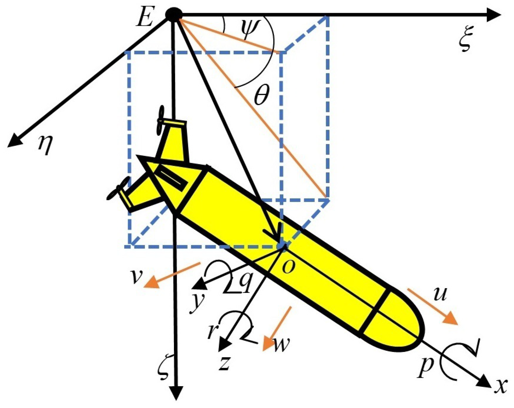
2.2. AUV Model on SO(3)

As shown in Figure 1, the attitude representation of an underactuated AUV is established in the Cartesian coordinate frame. The North-East-Down (NED) coordinate frame is denoted by $E-\eta \xi \zeta$. The body coordinate frame (B) is denoted by $o-xyz$. The attitude angle in NED is represented as ${\eta }_A={[\varphi ,\theta ,\psi ]}^{\top }$. $\varphi$ is the roll angle, $\theta$ is the pitch angle, and $\psi$ is the yaw angle. The angular velocity in the B frame is represented as $\omega ={[{\omega }_x,{\omega }_y,{\omega }_z]}^{\top }$. The kinematic equation of an underactuated AUV on SO(3) is represented as follows (see [8]).

$$\dot{R}=RS\left(\omega \right)$$

(6)

where the rotation matrix R is detailed as follows.

$$R=\left[\begin{array}{ccc}{c}_3{c}_2& c_3{s}_2{s}_1-s_3{c}_1& c_3{s}_2{c}_1+s_3{s}_1\\ s_3{c}_2& s_3{s}_2{s}_1+c_3{c}_1& s_3{s}_2{c}_1-c_3{s}_1\\ -s_2& c_2{s}_1& c_2{c}_1\end{array}\right]$$

(7)

$s(·)$ and $c(·)$ denote $sin\left(\right)$ and $cos\left(\right)$, respectively, and the subscripts $1,2$, and 3 represent the roll angle $\varphi$, the pitch angle $\theta$, and the yaw angle $\psi$, respectively.

In frame B, the attitude dynamic model of underactuated AUVs is described as follows (see [6]).

$$J\dot{\omega }+C(\nu ,\omega )\omega +D(\nu ,\omega )\omega +g\left({\eta }_A\right)=\tau +{\tau }_d$$

(8)

where $J=diag\left\{I_{xx}-K_{\dot{p}},I_{yy}-M_{\dot{q}},I_{zz}-N_{\dot{r}}\right\}$. $\nu ={[u,v,w]}^{\top }$ denotes the velocity in three directions along the B-frame. $C(\nu ,\omega )$ is described as follows:

$$C(\nu ,\omega )=\left[\begin{array}{ccc}0& -m{x}_{g}q+m_{11}w& -m{x}_{g}r-m_{22}v\\ m{x}_{g}q-m_{11}w& 0& -m_{33}p\\ m{x}_{g}r+m_{22}v& m_{33}p& 0\end{array}\right]$$

(9)

where m is the mass of the AUV; $m_{11},m_{22}$ and $m_{33}$ are the added mass parameters; and $x_g$ is the x-position of the center of gravity. $D\left(\nu \right)=diag\left\{K_p+K_{p\left|p\right|}\left|p\right|,M_q+\right.$$\left.M_{q\left|q\right|}\left|q\right|,N_r+N_{r\left|r\right|}\left|r\right|\right\}$. $g\left({\eta }_A\right)={[\left(z_{g}W\right)c\left(\theta \right)s\left(\varphi \right),\left(z_{g}W\right)s\left(\theta \right),0]}^{\top }$, where $z_g$ is the z-position of the center of gravity. $\tau \in {\mathbb{R}}^{3\times 1}$ represents the torque vector of underactuated AUVs. ${\tau }_d\in {\mathbb{R}}^{3\times 1}$ represents the external disturbance vector of underactuated AUVs.

2.3. Problem Formulation

This study focuses on the attitude stabilization control of underactuated AUVs in the vertical plane. The roll angle $\varphi$ of underactuated AUVs is uncontrollable; therefore, the torque corresponding to its roll angular velocity ${\omega }_x$ is zero. However, due to the presence of external disturbances and the coupling between angles, maintaining the roll angular velocity of underactuated AUVs at zero is difficult. Moreover, accurately obtaining the dynamic parameters of underactuated AUVs is difficult, so we can consider the matrices $C(\nu ,\omega )$, $D(\nu ,\omega )$, and $g\left({\eta }_A\right)$ as unknown terms of the AUV controllable models and the parameter matrix $J=J_0+J_u$, where $J_u$ is also unknown. Thus, the attitude controllable dynamic model can be rewritten as follows.

$$J_0\dot{\omega }=\tau +d$$

(10)

where $J_0\in {\mathbb{R}}^{2\times 2}$, $\omega ={[{\omega }_y,{\omega }_z]}^{\top }$, and $d\in {\mathbb{R}}^{2\times 1}$ represents the overall unknown terms of the model and is defined as $d=-C(\nu ,\omega )\omega -D(\nu ,\omega )\omega -g\left({\eta }_A\right)+{\tau }_d$. Without loss of generality, the assumption of this work is given.

Assumption 1.

The overall unknown terms d are bounded and unknown. Its derivatives are also bounded and unknown, that is, $\left|\right|d\left|\right|\le L_d$ and $\left|\right|\dot{d}\left|\right|\le L_{\dot{d}}$. $L_d$ and $L_{\dot{d}}$ are unknown positive constants.

Control goal: On the basis of Assumption 1, considering the saturation characteristics of the control input, we design the control input $\tau$ for the model (10) to practically stabilize its attitude angle, except for the roll angle $\varphi$. That is,

$$\underset{t\to \infty }{lim}\left|\right|\theta \left(t\right)-{\theta }_d\left|\right|\le {\epsilon }_{\theta },\underset{t\to \infty }{lim}\left|\right|\psi \left(t\right)-{\psi }_d\left|\right|\le {\epsilon }_{\psi }$$

(11)

where ${\theta }_d$ denotes the desired pitch angle and where ${\psi }_d$ denotes the desired yaw angle. ${\epsilon }_{\theta }$ and ${\epsilon }_{\psi }$ are two small positive constants. Notably, when the roll angle $\varphi$ changes, we cannot guarantee the asymptotic stabilization of the pitch angle $\theta$ and the yaw angle $\psi$, and there may be steady-state errors.

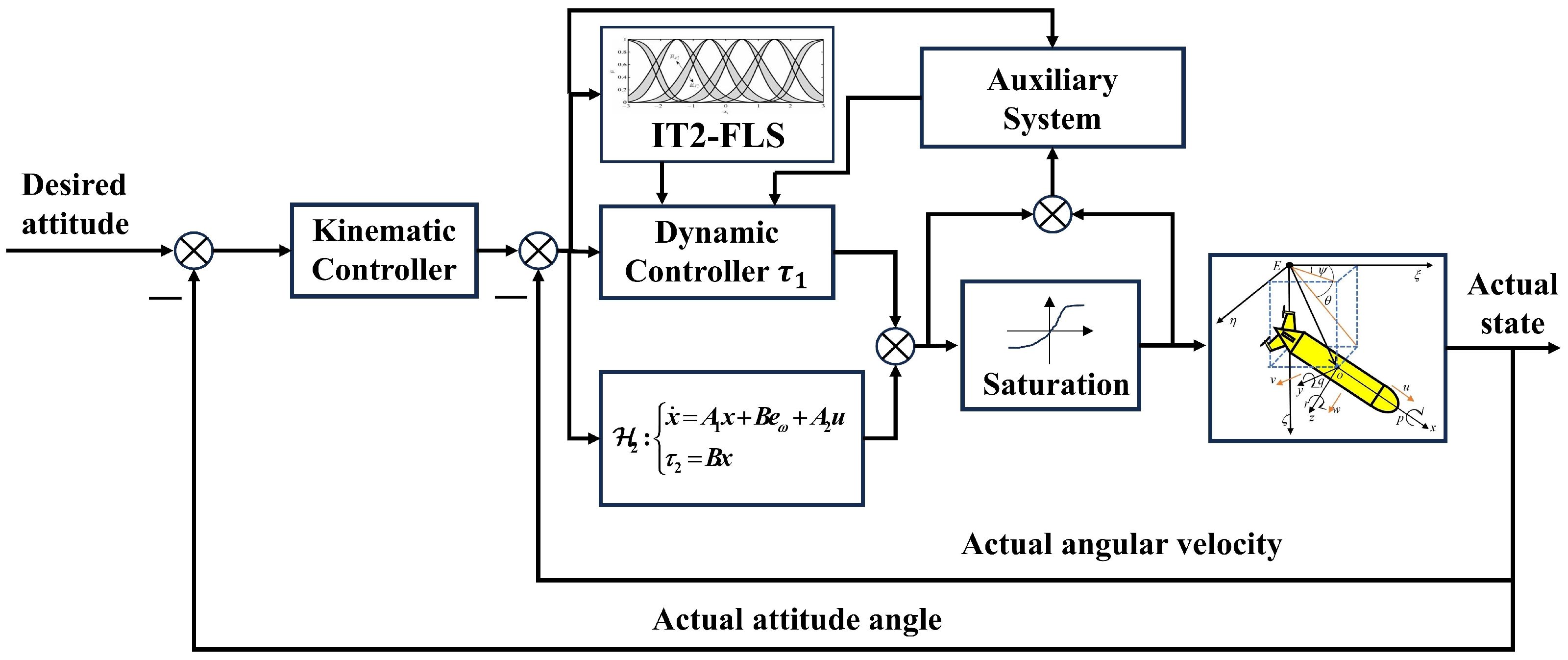
3. Controller Design and Stability Analysis

In this section, the first step is to design the kinematic controller based on transverse function. This can ensure that the attitude error is exponentially convergent. Next, the backstepping method is adopted to design the dynamic controller, and the unknown parts of the model are estimated by the IT2-FLS. The stability analysis of the attitude stabilization system is promising and is based on the small gain theorem. Finally, the saturation auxiliary system is designed to compensate for the saturation characteristics of the system control inputs. The closed-loop system diagram is shown in Figure 2.

3.1. Kinematic Controller That Is Based on the Transverse Function

The desired angle on SO(3) is defined as $R_d$; the desired angular velocity is ${\omega }_d$. The attitude error matrix can be described as $R_e=R_d^{\top }R$. The derivative of $R_e$ is taken as follows.

$${\dot{R}}_e=R_{e}S({\omega }_y{e}_2+{\omega }_z{e}_3+{\omega }_x{e}_1-R_e^{\top }{\omega }_d)$$

(12)

where ${\omega }_x$ is uncontrollable. The feasible trajectory of the attitude error equation is ${\omega }_x=e_1\left(R_e^{\top }{\omega }_d\right)$. According to [20], the transverse function of (12) is constructed as follows.

$$\begin{array}{cc}\hfill & f\left(\alpha \right)=exp(\epsilon sin\left(\alpha \right)S\left(e_2\right)+\epsilon cos\left(\alpha \right)S\left(e_3\right))\hfill \\ \hfill & =\left[\begin{array}{ccc}c\left(\epsilon \right)& -c\left(\alpha \right)s\left(\epsilon \right)& s\left(\alpha \right)s\left(\epsilon \right)\\ c\left(\alpha \right)s\left(\epsilon \right)& c^2\left(\alpha \right)c\left(\epsilon \right)+s^2\left(\alpha \right)& c\left(\alpha \right)s\left(\alpha \right)(1-c(\epsilon \left)\right)\\ -s\left(\alpha \right)s\left(\epsilon \right)& c\left(\alpha \right)s\left(\alpha \right)(1-c(\epsilon \left)\right)& s^2\left(\alpha \right)c\left(\epsilon \right)+c^2\left(\alpha \right)\end{array}\right]\hfill \end{array}$$

(13)

The transverse function is an embedded submanifold near a certain equilibrium point of the AUV attitude Lie group. Because underactuated AUVs have only two control variables, to solve the problem of three-dimensional state variables, an embedded submanifold is introduced to expand the dimension of the attitude manifold to ensure that the uncontrollable state is maintained near the equilibrium point. The transverse function $f\left(\alpha \right)$ is the matrix of rotation with $\epsilon$ angle about the unit axis ${[0,sin\left(\alpha \right),cos\left(\alpha \right)]}^{\top }$ and $\epsilon \in (0,2\pi )$. Furthermore, the derivative of $f\left(\alpha \right)$ is as follows:

$${\displaystyle \frac{df\left(\alpha \right)}{d\alpha }}=f\left(\alpha \right)S\left(\mathsf{\Omega }\right)$$

(14)

where $\mathsf{\Omega }={[1-cos\left(\epsilon \right),cos\left(\alpha \right)sin\left(\epsilon \right),sin\left(\alpha \right)sin\left(\epsilon \right)]}^{\top }$. When $f\left(\alpha \right)$ is called the transverse function of (12), the vectors $\mathsf{\Omega }$, $e_2$ and $e_3$ must be linearly independent, so $cos\left(\epsilon \right)\ne 1$. The matrix $f\left(\alpha \right)$ is invertible.

We define the new attitude error as $z=R_{e}f{\left(\alpha \right)}^{\top }f\left({\alpha }_d\right)$. Our goal is to design the desired angular velocities ${\omega }_y$, ${\omega }_z$ and $\dot{\alpha }$ to ensure that the matrix z converges to $I_{3\times 3}$, that is, let $R_e\to f{\left(\alpha \right)}^{\top }f\left({\alpha }_d\right)$. $\dot{\alpha }$ is a virtual kinematic control input. Hence, the parameter $\epsilon$ should be small enough to ensure that the attitude error meets the requirement of boundedness. The derivative of the variable z is taken as follows.

$$\begin{array}{cc}\hfill \dot{z}& =zS\left(\left(f{\left({\alpha }_d\right)}^{\top }f\left(\alpha \right)\right)({\omega }_y{e}_2+{\omega }_z{e}_3-\dot{\alpha }\mathsf{\Omega }+{\omega }_x{e}_1-R_e^{\top }{\omega }_d)\right)\hfill \\ \hfill & =zS(Eu+\mu )=zS\left(u_r\right)\hfill \end{array}$$

(15)

where the control input is denoted as $u={[{\omega }_y,{\omega }_z,\dot{\alpha }]}^{\top }$, and the unit axis vector is denoted as $E=f{\left({\alpha }_d\right)}^{\top }f\left(\alpha \right)[e_2,e_3,\mathsf{\Omega }]$ and $\mu =f{\left({\alpha }_d\right)}^{\top }f\left(\alpha \right)({\omega }_x{e}_1-R_e^{\top }{\omega }_d)$. The new input variable is denoted as $u_r=Eu+\mu$.

To avoid singularity, the exponential map is used to represent the attitude error. The rotation vector of z is defined as $\varrho$. $\widehat{\varrho }$ is the Lie algebra of z; that is, $z=exp\left(\widehat{\varrho }\right)$. The exponential format of the attitude error z is written as follows.

$$\dot{\varrho }=dex{p}^{-1}(-\varrho )u_r$$

(16)

The matrix $dex{p}^{-1}(-\varrho )$ is invertible if $\varrho$ is restricted within a ball $B_r=\left\{\varrho \in {\mathbb{R}}^3:\left|\right|\varrho \left|\right|\le \pi \right\}$. If $\varrho ={[0,0,0]}^{\top }$, we have $dex{p}^{-1}\left(\varrho \right)=I$.

Theorem 1.

For the attitude kinematic model (12) of underactuated AUVs, the kinematic control input u can be designed as $E^{-1}(-k_{1}dexp(-\varrho )\varrho -\mu )$, which can ensure the bounded exponential convergence of the attitude error.

Proof. 

We choose the Lyapunov candidate as $V_k={\displaystyle \frac{1}{2}}{\varrho }^{\top }\varrho$. The derivative of time is ${\dot{V}}_k={\varrho }^{\top }dex{p}^{-1}(-\varrho )u_r$. By substituting u into $u_r$, $u_r$ can be recast as $-dex{p}^{-1}(-\varrho )\varrho$. Therefore, the derivative of time satisfies ${\dot{V}}_k=-k_1{\varrho }^{\top }\varrho \le 0$, and the attitude error z is exponentially convergent. The actual attitude error converges to $f{\left(\alpha \right)}^{\top }f\left({\alpha }_d\right)$. Therefore, the attitude error is bounded exponential convergent. □

Remark 1.

The critical points can be calculated as $\varrho =\left\{0,\pm \pi \right\}$. It shows that $\varrho \in B_r=\left\{\varrho :\left|\right|\varrho \left|\right|\le \pi \right\}$ identify the true attitude error. Thus, the value of variable ϱ should be restricted to $[-\pi ,\pi ]$, when ${\varrho }^{\top }{u}_r>0$ and $\left|\right|\varrho \left|\right|\ge \pi +\delta$, $\varrho =\varrho -2\pi {\displaystyle \frac{\varrho }{\left|\right|\varrho \left|\right|}}$.

Remark 2.

To ensure convergence of the attitude, the selection of the parameter ε has a significant effect. By linearizing (15), the following equation can be obtained:

$$e_1^{\top }\dot{\overline{\alpha }}=-e_1^{\top }\left[S\left({\omega }_d\right)\right]\overline{\alpha }$$

(17)

where $\overline{\alpha }=\mathsf{\Omega }\left({\alpha }_d\right)(\alpha -{\alpha }_d)$. We define a new variable $y=e_1^{\top }\overline{\alpha }=(1-cos\left(\epsilon \right))(\alpha -{\alpha }_d)$, which equals zero if and only if $\alpha ={\alpha }_d$. Hence, the derivative of y is as follows:

$$\begin{array}{cc}\hfill \dot{y}& ={\displaystyle \frac{-e_1^{\top }\left[S\left({\omega }_d\right)\right]\mathsf{\Omega }\left({\alpha }_d\right)}{1-cos\left(\epsilon \right)}}y\hfill \\ \hfill & =({\omega }_{d3}cos\left({\alpha }_d\right)+{\omega }_{d2}sin\left({\alpha }_d\right))cot\left({\displaystyle \frac{\epsilon }{2}}\right)y\hfill \end{array}$$

(18)

For the convergence of the system (17), we select ${\alpha }_d={\displaystyle \frac{pi}{2}}$, so ε can be designed as follows:

$$\epsilon =-|{\epsilon }_r|sgn\left({\omega }_{d2}\right),{\epsilon }_r\in (0.2\ast pi)$$

(19)

3.2. Dynamic Controller Based on the Small Gain Theorem

In this section, we adopt the IT2-FLS to estimate the unknown parts of the model (10) and then combine the small gain theorem and the backstepping method to design a new robust attitude dynamic controller. On this basis, considering the saturation characteristic of the controller, a saturation auxiliary system is introduced to further modify the robust controller.

In Section 3.1, the kinematic control input $u\in {\mathbb{R}}^{3\times 1}$ is given. This includes the expected pitch angular velocity ${\omega }_y^d$, the expected yaw angular velocity ${\omega }_z^d$, and a virtual control input $\dot{\alpha }$. The variables ${\omega }_y^d$ and ${\omega }_z^d$ are the desired values of the model (10), that is, ${\omega }_d={[{\omega }_y^d,{\omega }_z^d]}^{\top }$. The error is defined as $e_{\omega }=\omega -{\omega }_d$. $\tau$ is divided into ${\tau }_1$ and ${\tau }_2$. ${\tau }_1$ ensures the practical stability of the underactuated AUVs’ attitudes, whereas ${\tau }_2$ is a robust compensation term used to improve the disturbance immunity of the attitude control. ${\tau }_2$ is designed as follows.

$$\left\{\begin{array}{c}\dot{x}=A_{1}x+B{e}_{\omega }+A_{2}u\hfill \\ {\tau }_2=Bx\hfill \end{array}\right.$$

(20)

where $A_1,A_2\in {\mathbb{R}}^{2\times 2}$ is a positive definite parameter matrix, $B\in {\mathbb{R}}^{2\times 2}$ is a unit matrix, and u is an auxiliary input variable.

Theorem 2.

For the underactuated AUV model (10), the controller is designed as ${\tau }_1=-k_3{e}_{\omega }-{\widehat{\mathsf{\Theta }}}^{\top }\xi +J_0{\dot{\omega }}_d$, the robust controller input ${\tau }_2$ is designed as (20), the auxiliary input $u=-2A_2^{-1}{A}_{1}x$, and the IT2-FLS updating law is designed as $\dot{\widehat{\mathsf{\Theta }}}=-2\beta \widehat{\mathsf{\Theta }}+e_{\omega }^{\top }\xi$; these can ensure that the attitude system is ISPS, where $\widehat{\mathsf{\Theta }}$ and ξ are the weight vector and the basis function of the IT2-FLS, respectively, and $k_3,\beta \in {\mathbb{R}}^{2\times 2}$ are positive definite matrices.

Proof. 

The attitude control system can be established as two interconnection systems ${\mathcal{H}}_1$ and ${\mathcal{H}}_2$ as follows:

$$\begin{array}{c}{\mathcal{H}}_1:\left\{\begin{array}{c}{\dot{e}}_{\omega }=J_0^{-1}({\tau }_1+{\tau }_2+d)-{\dot{\omega }}_d\hfill \\ y_1=e_{\omega }\hfill \end{array}\right.\hfill \\ {\mathcal{H}}_2:\left\{\begin{array}{c}\dot{x}=A_{1}x+B{e}_{\omega }+A_{2}u\hfill \\ {\tau }_2=Bx\hfill \end{array}\right.\hfill \end{array}$$

(21)

For the system ${\mathcal{H}}_1$, we choose the Lyapunov candidate as $V_1={\displaystyle \frac{1}{2}}{e}_{\omega }^{\top }{J}_0{e}_{\omega }+{\displaystyle \frac{1}{2}}{\tilde{\mathsf{\Theta }}}^{\top }\tilde{\mathsf{\Theta }}$, where $\tilde{\mathsf{\Theta }}=\mathsf{\Theta }-\widehat{\mathsf{\Theta }}$. Taking its derivative as follows.

$${\dot{V}}_1=e_{\omega }^{\top }{\tau }_1+e_{\omega }^{\top }{\tau }_2+e_{\omega }^{\top }{\mathsf{\Theta }}^{\top }\xi -e_{\omega }^{\top }{J}_0{\dot{\omega }}_d-{\tilde{\mathsf{\Theta }}}^{\top }\dot{\widehat{\mathsf{\Theta }}}$$

(22)

Substituting ${\tau }_1$ and $\dot{\widehat{\mathsf{\Theta }}}$ into (22) and $2\beta {\tilde{\mathsf{\Theta }}}^{\top }\widehat{\mathsf{\Theta }}={\beta \left|\right|\mathsf{\Theta }\left|\right|}^{ 2}-\beta \left|\right|\widehat{\mathsf{\Theta }}{\left|\right|}^2-\beta \left|\right|\tilde{\mathsf{\Theta }}{\left|\right|}^2$, the result can be recast as follows.

$${\dot{V}}_1\le -k_3\left|\right|e_{\omega }{\left|\right|}^2-\beta \left|\right|\tilde{\mathsf{\Theta }}{\left|\right|}^2+e_{\omega }^{\top }{\tau }_2+{\beta \left|\right|\mathsf{\Theta }\left|\right|}^{ 2}$$

(23)

Because ${\tau }_2=y_2$ and $\mathsf{\Theta }$ can be used as the external input, the following must hold.

$${\dot{V}}_1\le -{\lambda }_s\left(K\right)V_1+{\displaystyle \frac{1}{2\vartheta }}\left|\right|y_2{\left|\right|}^2+{\beta \left|\right|\mathsf{\Theta }\left|\right|}^{ 2}$$

(24)

where $K=diag\left\{(k_3-{\displaystyle \frac{\vartheta }{2}}),\beta \right\}$. Integrating the above equation in the interval of $[0,t]$ is easy to obtain as follows:

$$\begin{array}{cc}\hfill V_1\left(t\right)& \le e^{-2{\lambda }_s\left(K\right)t}{V}_1\left(0\right)+{\displaystyle \frac{1}{2\vartheta }}{\int }_0^t{e}^{-2{\lambda }_s\left(K\right)(t-\tau ))}\left|\right|y_2{\left|\right|}^{2}d\tau \hfill \\ \hfill & +{\int }_0^t{e}^{-2{\lambda }_s\left(K\right)(t-\tau ))}{\left|\right|\mathsf{\Theta }\left|\right|}^{ 2}d\tau \hfill \end{array}$$

(25)

The square root of the above equation is calculated to obtain

$$\left|\right|e_{\omega }\left|\right|\le e^{-{\lambda }_s\left(K\right)t}\left|\right|e_{\omega }\left(0\right)\left|\right|+{\displaystyle \frac{1}{\sqrt{2\vartheta }}}c\left|\right|y_2\left|\right|+\sqrt{k_2}c\left|\right|\mathsf{\Theta }\left|\right|$$

(26)

where $c=\sqrt{{\displaystyle \frac{1-e^{-2{\lambda }_s\left(K\right)t}}{2{\lambda }_s\left(K\right)}}}$. The ${\mathcal{H}}_1$ system is ISPS.

For system ${\mathcal{H}}_2$, we choose the Lyapunov candidate $V_2={\displaystyle \frac{1}{2}}{x}^{\top }x$. By performing derivative calculations, we can also obtain the following:

$$\left|\right|x\left|\right|\le e^{-{\lambda }_s(A_1-{\displaystyle \frac{\vartheta }{2}})}\left|\right|x\left(0\right)\left|\right|+{\displaystyle \frac{1}{\sqrt{2\vartheta }}}c\left|\right|y_1\left|\right|$$

(27)

Therefore, the following inequality must hold:

$$\left|\right|y_2\left|\right|\le {\lambda }_b\left(B\right)e^{-{\lambda }_s(A_1-{\displaystyle \frac{\vartheta }{2}})t}\left|\right|x\left(0\right)\left|\right|+{\displaystyle \frac{{\lambda }_b\left(B\right)}{\sqrt{2\vartheta }}}c\left|\right|y_1\left|\right|$$

(28)

The ${\mathcal{H}}_2$ system is ISPS(ISS). For system ${\mathcal{H}}_1$, ${\alpha }_3\left(s\right)={\lambda }_s\left(K\right)s^2$, ${\alpha }_4\left(s\right)={\displaystyle \frac{1}{2\vartheta }}{s}^2$, and there exist ${\alpha }_1\left(s\right)$ and ${\alpha }_2\left(s\right)$ that are $K_{\infty }$ functions. Its gain is ${\gamma }_{{\mathcal{H}}_1}={\alpha }_1^{-1}\circ {\alpha }_2\circ {\alpha }_3^{-1}\circ {\alpha }_4\left(s\right)$. For system ${\mathcal{H}}_2$, ${\alpha }_3\left(s\right)={\lambda }_s\left(A\right)s^2$, ${\alpha }_4\left(s\right)={\displaystyle \frac{1}{2\vartheta }}{s}^2$, and there exist ${\alpha }_1\left(s\right)$ and ${\alpha }_2\left(s\right)$ that are $K_{\infty }$ functions. Its gain is ${\gamma }_{{\mathcal{H}}_2}={\alpha }_1^{-1}\circ {\alpha }_2\circ {\alpha }_3^{-1}\circ {\alpha }_4\left(s\right)$. According to Definitions 1 and 2, when the overall control parameters satisfy $2\vartheta {\lambda }_s^2\left(K\right)\le {\lambda }_s\left(A\right)$, the entire system is ISPS. □

3.3. Dynamic Controller with Input Saturation

Considering the impact of control input saturation characteristics on system performance, this section introduces a saturation auxiliary system to compensate for this effect. The auxiliary system is designed as follows:

$$\dot{\lambda }=\left\{\begin{array}{c}-K_{\lambda }\lambda -(e_{\omega }^{\top }\Delta \tau /{\left|\right|\lambda \left|\right|}^2)\lambda +e_{\omega }|\Delta \tau |\ne 0\hfill \\ e_{\omega }|\Delta \tau |=0\hfill \end{array}\right.$$

(29)

where $\Delta \tau$ denotes the error of the control input, that is, $\Delta =sat\left(\tau \right)-\tau$, $\lambda$ represents the state variable of the auxiliary system, and $K_{\lambda }\in {\mathbb{R}}^{2\times 2}$ denotes the gain parameter.

Remark 3.

In $|\Delta \tau |\ne 0$, the denominator has no solution when $\lambda =0$. To avoid unsolvable situations, when $\left|\lambda \right|<ϵ$,$\dot{\lambda }=0$. When $\left|\lambda \right|\ge ϵ$, $\dot{\lambda }$ is still (29). ϵ is a small positive constant.

Theorem 3.

Considering the saturation characteristics of the control input, the controller is designed as ${\tau }_1=-k_3{e}_{\omega }-{\widehat{\mathsf{\Theta }}}^{\top }\xi +J_0{\dot{\omega }}_d-\lambda$, the robust controller input ${\tau }_2$ is designed as (20), the auxiliary input $u=-2A_2^{-1}{A}_{1}x$, the IT2-FLS updating law is designed as $\dot{\widehat{\mathsf{\Theta }}}=-2\beta \widehat{\mathsf{\Theta }}+e_{\omega }^{\top }\xi$, and the saturation auxiliary system is designed as (29), which can ensure that the attitude stabilization is practically asymptotically stable.

Proof. 

We choose the Lyapunov candidate as $V={\displaystyle \frac{1}{2}}{e}_{\omega }^{\top }{e}_{\omega }+{\displaystyle \frac{1}{2}}{\tilde{\mathsf{\Theta }}}^{\top }\tilde{\mathsf{\Theta }}+{\displaystyle \frac{1}{2}}{x}^{\top }x+{\displaystyle \frac{1}{2}}{\lambda }^{\top }\lambda$. The control input is $\tau ={\tau }_1+{\tau }_2$. When $\Delta \tau \ne 0$ and $\left|\lambda \right|>ϵ$, we take its derivative of time and substitute $\tau$, the updating laws, and (29) into the result, which can be written as follows:

$$\begin{array}{cc}\hfill \dot{V}& \le -k_3\left|\right|e_{\omega }{\left|\right|}^2-\beta \left|\right|\tilde{\mathsf{\Theta }}{\left|\right|}^2-{\lambda }_s\left(A_1\right){\left|\right|x\left|\right|}^2-K_{\lambda }{\left|\right|\lambda \left|\right|}^2\hfill \\ \hfill & +{\beta \left|\right|\mathsf{\Theta }\left|\right|}^{ 2}+2{\lambda }_b\left(B\right)\left|x\right||e_{\omega }|\hfill \\ \hfill & \le -(k_3-{\lambda }_s\left(B\right))\left|\right|e_{\omega }{\left|\right|}^2-\beta \left|\right|\tilde{\mathsf{\Theta }}{\left|\right|}^2-K_{\lambda }{\left|\right|\lambda \left|\right|}^2\hfill \\ \hfill & -({\lambda }_s\left(A_1\right)-{\lambda }_s\left(B\right)){\left|\right|x\left|\right|}^2+{\beta \left|\right|\mathsf{\Theta }\left|\right|}^{ 2}\hfill \end{array}$$

(30)

When $\Delta \tau =0$ and $\left|\lambda \right|>ϵ$, the derivative of the Lyapunov V is as follows:

$$\begin{array}{cc}\hfill \dot{V}& \le -(k_3-{\lambda }_s\left(B\right))\left|\right|e_{\omega }{\left|\right|}^2-({\lambda }_s\left(A_1\right)-{\lambda }_s\left(B\right)){\left|\right|x\left|\right|}^2\hfill \\ \hfill & -\beta \left|\right|\tilde{\mathsf{\Theta }}{\left|\right|}^2+{\beta \left|\right|\mathsf{\Theta }\left|\right|}^{ 2}\hfill \end{array}$$

(31)

When $\left|\lambda \right|<ϵ$, the system tends to stabilize, and $|\Delta \tau |=0$. Hence, the derivative of the Lyapunov V is as follows.

$$\begin{array}{cc}\hfill \dot{V}& \le -(k_3-{\lambda }_s\left(B\right)-{\displaystyle \frac{1}{2}})\left|\right|e_{\omega }{\left|\right|}^2-({\lambda }_s\left(A_1\right)-{\lambda }_s\left(B\right)){\left|\right|x\left|\right|}^2\hfill \\ \hfill & -\beta \left|\right|\tilde{\mathsf{\Theta }}{\left|\right|}^2+{\beta \left|\right|\mathsf{\Theta }\left|\right|}^{ 2}+{\displaystyle \frac{1}{2}}{\left|ϵ\right|}^2\hfill \end{array}$$

(32)

When the system is in the adjustment process, on the basis of (30), we define $A=diag\left((k_3-{\lambda }_s\left(B\right)),\beta ,({\lambda }_s\left(A_1\right)-{\lambda }_s\left(B\right)),K_{\lambda }\right)$ and integrate (30) from 0–t; the result can be obtained as follows:

$$\left|\right|p\left|\right|\le e^{-{\lambda }_s\left(A\right)t}\left|\right|p\left(0\right)\left|\right|+\sqrt{\beta }c\left|\right|\mathsf{\Theta }\left|\right|$$

(33)

where $c=\sqrt{{\displaystyle \frac{1-e^{-2{\lambda }_s\left(A\right)t}}{2{\lambda }_s\left(A\right)}}}$, $p={[e_{\omega },\tilde{\mathsf{\Theta }},x,\lambda ]}^{\top }$. Therefore, vector p is bounded and exhibits exponential convergence. The convergence speed is related to matrix A, and the final convergence bound is determined by the initial state and $\mathsf{\Theta }$. When $\left|\lambda \right|<ϵ$, $K_{\lambda }=0$, the system error is also bounded and satisfies

$$\left|\right|p\left|\right|\le e^{-{\lambda }_s\left(A\right)t}\left|\right|p\left(0\right)\left|\right|+\sqrt{\beta }c\left|\right|\mathsf{\Theta }\left|\right|+{\displaystyle \frac{1}{\sqrt{2}}}c\left|\right|ϵ\left|\right|$$

(34)

In summary, the system error is bounded and directly related to the initial state. The closed-loop system is ISPS. The steady-state error of the system is caused by two factors. The first factor is the introduction of the transverse function in the kinematic controller (Theorem 1), where the parameter $\epsilon$ of the transverse function cannot be zero, resulting in a small error in the attitude error z. The second factor is due to the introduction of the dynamic controller (20). By using the Lyapunov theorem to prove the stability of the system, the error inequality (34) can be obtained. The overall system error must satisfy $\left|\right|p\left|\right|\le k\left|\right|p\left(0\right)\left|\right|+\delta$, where $k=e^{-{\lambda }_s\left(A\right)t}$ and $\delta$ is a bounded small constant. □

4. Simulation Results

To verify the effectiveness and robustness of the proposed controller, simulation verification is conducted, and the results are compared with those of [21,23]. The proposed controller in [21] is called “Comparison 1”, and the proposed controller in [23] is called “Comparison 2”. The simulation object is the “REMUS100” underactuated AUV, and its hydrodynamic parameters are listed in Appendix A. The compared controllers in [21] are as follows.

$$\tau =-C\omega -D\omega -g-A^{-1}{f}_d^{\top }(k_1{u}_r+k_2{\nu }_R+f_d\mathsf{\Phi })$$

(35)

where ${\nu }_R={\displaystyle \frac{{(z-z^{\top })}^{\vee }}{2\sqrt{1+tr\left(z\right)}}}$, $\mathsf{\Phi }=2-\sqrt{1+tr\left(z\right)}$, $k_1=diag\left\{0.21,0.21,0.07\right\}$ and $k_2=diag\left\{12.4,23.5\right\}$. The simulation step is 0.1 s, and the simulation time is 800 s. The initial angle of the AUV is set as $\theta \left(0\right)=0^{\circ }$ and $\psi \left(0\right)=0^{\circ }$. The initial angular velocity is ${\omega }_y\left(0\right)=0$ rad/s, and ${\omega }_z\left(0\right)=0$ rad/s. The initial $\alpha \left(0\right)=0.15$ rad, the initial weight vectors $\mathsf{\Theta }\left(0\right)$ and the basis function vectors $\xi \left(0\right)$ are random numbers in $(0,1)$. The initial state $\lambda \left(0\right)$ of the auxiliary system is set as 1 and $x\left(0\right)=0$. ${\omega }_d={[0,0,0]}^{\top }$. The input boundary for controlling torque is $[-15,15]$ N/m. The disturbance vector dis is set as follows:

$$dis=\left[\begin{array}{c}-0.1sin\left(0.02\pi t\right)+0.2cos\left(0.02\pi t\right)\\ 0.2sin\left(0.02\pi t\right)-0.3cos\left(0.02\pi t\right)\\ -0.2sin\left(0.02\pi t\right)+0.1cos\left(0.02\pi t\right)\end{array}\right]$$

4.1. Selection of the Controller Parameters

On the basis of (19), we select ${\alpha }_d={\displaystyle \frac{\pi }{2}}$, and the parameter ${\epsilon }_r$ is selected as $0.8$. According to (33) and (34), to obtain faster response speed, the minimum eigenvalue of matrix A should be sufficiently small. However, to minimize the margin of error, the parameters c and $\beta$ should be smaller; that is, the minimum eigenvalue of matrix A should be sufficiently large. To solve the steady-state error of this method, we strive to ensure that the initial state is not significantly different from the expected state as much as possible and that the selection of controller parameter A should be as large as possible to reduce the impact of the initial state on the errors. However, excessively large parameters can slow the response speed of the system. Meanwhile, the transverse function parameter $\epsilon$ should be kept as small as possible and can be chosen to be approximately 0.01. Hence, the parameters $k_3$, $A_1$, B, and $K_{\lambda }$ should be chosen eclectically.

Table 1. The controller parameter selection in the simulation.

Parameters	Value
	Pitch Channel	Yaw Channel
$A_1$	10	10
B	1	1
$K_{\lambda }$	2	2
$k_1$	0.15	0.11
$k_3$	23.5	22.5
$\beta$	0.2	0.2
$ϵ$	0.01	0.01

shows the selection of the parameters.

The basis function of the IT2-FLS is as follows:

$$\begin{array}{cc}\hfill & {\mu }_{F_{\phi }^{UMF}}^i=exp(-{\left({\displaystyle \frac{\phi -m_{\phi 1}+m_{\phi 2}i}{m_{\phi 3}}}\right)}^2)\hfill \\ \hfill & {\mu }_{F_{\phi }^{UMF}}^i=exp(-{\left({\displaystyle \frac{\phi -m_{\phi 4}+m_{\phi 2}5}{m_{\phi 6}}}\right)}^2)\hfill \end{array}$$

where $\phi$ denotes the state of the AUV and $\phi ={[p,q,r,\varphi ,\theta ]}^{\top }$; $m_{\phi 1,4}=[1,1,0.2,2\pi ,\pi ]$, $m_{\phi 2,5}=[0.5,0.5,0.1,\pi ,\pi /2]$, and $m_{\phi 3,6}=[0.25,0.25,0.05,\pi /2,\pi /4]$.

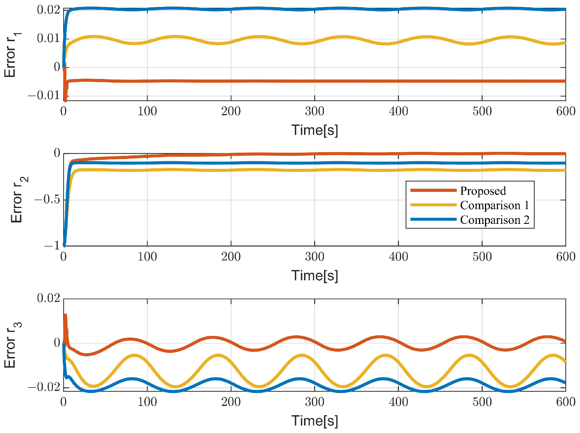
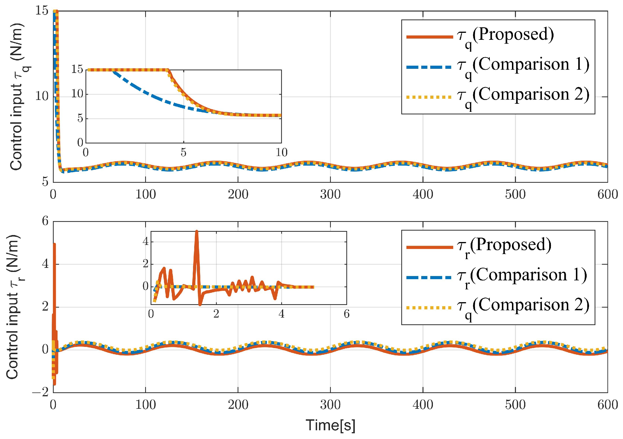
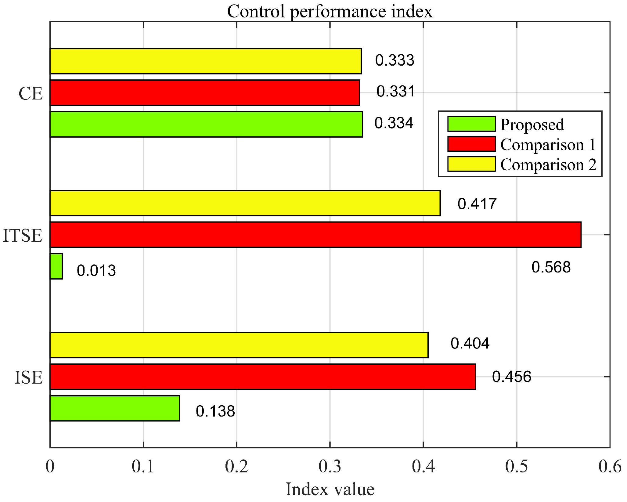
4.2. Controller Performance Verification

This section validates the performance of the proposed controller via two different underwater task scenarios. We use three metrics to evaluate the performance of the controller: the integral of square error (ISE) $J_1={\int }_0^{T}t{e}^2\left(t\right)dt$, the integral of time square error (ITSE) $J_2={\int }_0^{T}te{\left(t\right)}^{2}dt$, and the controller energy (CE) $J_3={\int }_0^{t}u{\left(t\right)}^{2}dt$. ISE is used to evaluate the response speed and stability, ITSE is used to evaluate the steady-state error, and CE is used to evaluate the control input energy consumption. However, there is a significant difference in the magnitude of the three indicators. Therefore, we normalize the results. For example, result = ISE1/(ISE1 + ISE2 + ISE3). Among them, ISE1 represents the ISE of the proposed controller, ISE2 is the ISE of the Comparison 1 method, and ISE3 is the ISE of the Comparison 2 method. Other indicators are also calculated in the same way. The smaller the performance indicators of the corresponding controllers are, the better the controller is.

4.2.1. Scenario 1

At present, the use of Euler angles for the vertical diving attitude control of AUVs exhibits singularity. The proposed controller can meet the task requirements of AUV vertical diving. Therefore, the desired attitude angle is set as ${\theta }_d={90}^{\circ }$ and ${\psi }_d=0^{\circ }$.

Our goal is to make the error attitude rotation matrix $R_e$ equal to the identity matrix $I_{3\times 3}$ and the matrix $R_e\approx I+S\left(r\right)$. When vector r is equal to zero, $R_e\approx I$. Hence, we use vector r to represent the attitude error. Figure 3 shows the attitude stabilization errors of the proposed controller and the controller in [21,23]. Although the comparison methods can converge quickly, they have larger steady-state errors. The proposed controller can converge the attitude error to a certain range in the presence of an external disturbance and an unknown model. This further proves that the controller is practically exponentially stable. Figure 4 shows the control input of the two controllers. Under the influence of disturbances, the controller is continuously adjusted. In the initial stage, the proposed controller input is only in a saturation state for 2 s, whereas the saturation state of the Comparison 1 controller lasts for 7 s.

Figure 5 compares the indicators of the three controllers. Based on the analysis of ISE, ITSE, and CE, we can conclude that the proposed controller outperforms the compared algorithms in terms of response speed, steady-state error, system stability, and robustness. In terms of energy consumption, there is not much difference between the two methods.

Figure 6 and Figure 7 show the IT2-FLS weight vectors, and the auxiliary system state $\lambda$ can quickly converge to a stable value. Figure 8 shows that the proposed controller can ensure a sufficiently small range of attitude changes near the desired attitude, that is, achieve practical attitude stabilization. Figure 9 shows the motion trajectory of the underactuated AUV in vertical diving.

4.2.2. Scenario 2

To further verify the effectiveness of the controller, an underwater operation scenario with continuous attitude changes is designed, and the desired attitude design is

$${\theta }_d=\left\{\begin{array}{c}{75}^{\circ }0\mathrm{s}\le t\le 500\mathrm{s}\hfill \\ -{75}^{\circ }200\mathrm{s}<t\le 500\mathrm{s}\hfill \end{array}\right.$$

${\psi }_d=0^{\circ }$. The simulation time is 1000 s.

Figure 10 shows the attitude stabilization error. The proposed controller can ensure that the underactuated AUV completes attitude switching smoothly and maintains a sufficiently small steady-state error. Figure 11 shows the control input curves. As the disturbance changes, the control input also constantly changes. At the moment of attitude switching, the control input undergoes a sudden change and quickly converges. Figure 12 shows the comparison results of three indicators. For ISE and ITSE, the proposed controller performs better, and its response speed, stability, and robustness are better than those of the comparison methods. In terms of the CE indicator, there is not much difference.

Figure 13 and Figure 14 show the convergence of the IT2-FLS weight vectors and auxiliary system state $\lambda$. They can achieve good convergence to a fixed value. Figure 15 shows the quaternion of the underactuated AUV. The proposed controller has a smaller steady error than the comparison method does; even for more complex attitude switching tasks, this method can still ensure practical stabilization of the AUV attitude. Figure 16 shows the motion trajectory of the underactuated AUV in this scenario.

In the subsequent experiments, our experimental subject is a 20-kilogram small AUV. It is equipped with four thrusters that can control five degrees of freedom except for roll. We first conduct controller testing on the AUV within a small pitch angle range (−45 degrees∼45 degrees) in the vertical plane, completing two consecutive small-scale continuous profiles. Afterwards, the AUV’s profile observation control capability will be tested with a large pitch angle. Like in scenario 2, the expected pitch angle is set to ±75 degrees, and two profile observation missions are completed. Finally, the control capability of vertical ascent and descent in simulation scenario 1 is tested. All the above tests analyze the stability, stability error, and robustness of the controller separately. Among them, robustness testing is conducted in the wave-making pool.

5. Conclusions

To avoid the singularity of Euler angles and the ambiguity of quaternions, this study adopts $SO\left(3\right)$ and designs the transverse function of the attitude to solve the attitude control problem of underactuated AUVs. To avoid the unsolvable phenomenon of traditional error functions, the exponential mapping of $SO\left(3\right)$ is used to design attitude kinematic controllers. IT2-FLS is used to approximate model uncertainty and ocean current disturbances. Moreover, to improve the robustness of the system, the small gain theorem is adopted to design the dynamic controller and ensure the practical input–output stability of the system. A new saturation auxiliary dynamic system is designed to compensate for the impact of actuator saturation characteristics. Finally, simulations in two different scenarios confirmed that the proposed controller can ensure the practical attitude stabilization of underactuated AUVs. However, this method has steady-state errors, and the errors are related to the initial state. In the future, we will conduct field experiments to validate this method and achieve asymptotic convergence of the system. We will also improve the transverse function (13) to make it an invertible matrix in all cases, such as when auxiliary variables are used. Moreover, the form of the dynamic controller (20) will be further modified such that its stability is no longer related to the initial error state.

References

1. Richmond, K.; Flesher, C.; Tanner, N.; Siegel, V.; Stone, W.C. Autonomous exploration and 3-D mapping of underwater caves with the human-portable SUNFISH® AUV. In Proceedings of the Global Oceans 2020: Singapore—U.S. Gulf Coast, Biloxi, MS, USA, 5–30 October 2020. [Google Scholar] [CrossRef]
2. Byron, J.; Tyce, R. Designing a vertical/horizontal AUV for deep ocean sampling. In Proceedings of the 2007 OCEANS, Vancouver, BC, Canada, 29 September–4 October 2007; pp. 1299–1308. [Google Scholar]
3. Liu, Z.; Cai, W.; Zhang, M.; Lv, S. Improved Integral Sliding Mode Control-Based Attitude Control Design and Experiment for High Maneuverable AUV. J. Mar. Sci. Eng. 2022, 10, 795. [Google Scholar] [CrossRef]
4. Xu, R.; Tang, G.; Han, L.; Huang, H.; Xie, D. Robust Finite-Time Attitude Tracking Control of a CMG-Based AUV With Unknown Disturbances and Input Saturation. IEEE Access 2019, 7, 56409–56422. [Google Scholar] [CrossRef]
5. Liu, X.; Zhang, M.; Chen, J.; Yin, B. Trajectory tracking with quaternion-based attitude representation for autonomous underwater vehicle based on terminal sliding mode control. Appl. Ocean Res. 2020, 104, 102342. [Google Scholar] [CrossRef]
6. Fjellstad, O.; Fossen, T. Position and attitude tracking of auvs—A quaternion feedback approach. IEEE J. Ocean. Eng. 1994, 19, 512–518. [Google Scholar] [CrossRef]
7. Zhu, C.; Huang, B.; Su, Y.; Zheng, Y.; Zheng, S. Finite-time rotation-matrix-based tracking control for autonomous underwater vehicle with input saturation and actuator faults. Int. J. Robust Nonlinear Control 2022, 32, 2925–2949. [Google Scholar] [CrossRef]
8. Zhang, Z.; Xu, Y.; Wan, L.; Chen, G.; Cao, Y. Rotation matrix-based finite-time trajectory tracking control of AUV with output constraints and input quantization. Ocean Eng. 2024, 293, 116570. [Google Scholar] [CrossRef]
9. Chaturvedi, N.A.; Sanyal, A.K.; McClamroch, N.H. Rigid-Body Attitude Control using rotation matrices for continuous, singularity-free control laws. IEEE Control Syst. Mag. 2011, 31, 30–51. [Google Scholar] [CrossRef]
10. Ferreira, B.M.; Jouffroy, J.; Matos, A.C.; Cruz, N.A. Control and guidance of a hovering AUV pitching up or down. In Proceedings of the 2012 OCEANS, Hampton Roads, VA, USA, 14–19 October 2012. [Google Scholar]
11. Gavrilina, E.; Chestnov, V. Singularity-Free Attitude Control of the Unmanned Underwater Vehicle. In Proceedings of the 2020 24th International Conference on System Theory, Control and Computing (ICSTCC), Sinaia, Romania, 8–10 October 2020; pp. 512–519. [Google Scholar] [CrossRef]
12. Bhat, S.; Bernstein, D. A topological obstruction to continuous global stabilization of rotational motion and the unwinding phenomenon. Syst. Control Lett. 2000, 39, 63–70. [Google Scholar] [CrossRef]
13. Huang, Z.; Su, Z.; Huang, B.; Song, S.; Li, J. Quaternion-based finite-time fault-tolerant trajectory tracking control for autonomous underwater vehicle without unwinding. ISA Trans. 2022, 131, 15–30. [Google Scholar] [CrossRef]
14. Su, Z.; Lin, X.; Huang, B.; Zhao, D.; Sun, H. Improved dynamic event-triggered anti-unwinding control for autonomous underwater vehicles. Ocean Eng. 2023, 272, 113619. [Google Scholar] [CrossRef]
15. Brockett, R.W. Asymptotic Stability and Feedback Stabilization, Differential Geometric Control Theory. Prog. Math. 1983, 27, 181–191. [Google Scholar]
16. Li, Y.; Li, Y.; Wu, Q. Design for three-dimensional stabilization control of underactuated autonomous underwater vehicles. Ocean Eng. 2018, 150, 327–336. [Google Scholar] [CrossRef]
17. Akhtar, A.; Waslander, S.L. Controller Class for Rigid Body Tracking on SO(3). IEEE Trans. Autom. Control 2021, 66, 2234–2241. [Google Scholar] [CrossRef]
18. Yu, Y.; Ding, X. A Global Tracking Controller for Underactuated Aerial Vehicles: Design, Analysis, and Experimental Tests on Quadrotor. IEEE-ASME Trans. Mechatron. 2016, 21, 2499–2511. [Google Scholar] [CrossRef]
19. Zhu, C.; Jun, L.; Huang, B.; Su, Y.; Zheng, Y. Trajectory tracking control for autonomous underwater vehicle based on rotation matrix attitude representation. Ocean Eng. 2022, 252, 111206. [Google Scholar] [CrossRef]
20. Morin, P.; Samson, C. Practical stabilization of driftless systems on Lie groups: The transverse function approach. IEEE Trans. Autom. Control 2003, 48, 1496–1508. [Google Scholar] [CrossRef]
21. Gui, H.; Vukovich, G.; Xu, S. Attitude Tracking of a Rigid Spacecraft Using Two Internal Torques. IEEE Trans. Aerosp. Electron. Syst. 2015, 51, 2900–2913. [Google Scholar] [CrossRef]
22. Sun, Y.; Liu, M.; Qin, H.; Wang, H.; Ding, Z. Full prescribed performance trajectory tracking control strategy of autonomous underwater vehicle with disturbance observer. ISA Trans. 2024, 151, 117–130. [Google Scholar] [CrossRef]
23. Wang, Y.; Li, Y.; Li, L. Trajectory tracking control of underwater vehicle considering state constraint and actuator saturation. Control Decis. 2024, 39, 1778–1786. [Google Scholar] [CrossRef]
24. Li, J.; Du, J.; Chen, C.L.P. Command-Filtered Robust Adaptive NN Control With the Prescribed Performance for the 3-D Trajectory Tracking of Underactuated AUVs. IEEE Trans. Neural Netw. Learn. Syst. 2022, 33, 6545–6557. [Google Scholar] [CrossRef]
25. Zhang, J.; Xiang, X.; Zhang, Q.; Li, W. Neural network-based adaptive trajectory tracking control of underactuated AUVs with unknown asymmetrical actuator saturation and unknown dynamics. Ocean Eng. 2020, 218, 108193. [Google Scholar] [CrossRef]
26. Yu, C.; Xiang, X.; Wilson, P.A.; Zhang, Q. Guidance-Error-Based Robust Fuzzy Adaptive Control for Bottom Following of a Flight-Style AUV With Saturated Actuator Dynamics. IEEE Trans. Cybern. 2020, 50, 1887–1899. [Google Scholar] [CrossRef] [PubMed]
27. Liang, X.; Wan, L.; Blake, J.I.R.; Shenoi, R.A.; Townsend, N. Path Following of an Underactuated AUV Based on Fuzzy Backstepping Sliding Mode Control. Int. J. Adv. Robot. Syst. 2016, 13, 122. [Google Scholar] [CrossRef]
28. Thanh, P.N.N.; Thuyen, N.A.; Anh, H.P.H. Adaptive fuzzy 3-D trajectory tracking control for autonomous underwater vehicle (AUV) using modified integral barrier lyapunov function. Ocean Eng. 2023, 283, 115027. [Google Scholar] [CrossRef]
29. Wang, H.D.; Zhai, Y.X.; Shah, U.H.; Karkoub, M.; Li, M. Adaptive fuzzy control of underwater vehicle manipulator system with dead-zone band input nonlinearities via fuzzy performance and disturbance observers. Ocean Eng. 2023, 277, 114194. [Google Scholar] [CrossRef]
30. Zadeh, L. The concept of a linguistic variable and its application to approximate reasoning. III. Inf. Sci. 1975, 9, 43–80. [Google Scholar] [CrossRef]
31. Liang, Q.; Mendel, J. Interval type-2 fuzzy logic systems: Theory and design. IEEE Trans. Fuzzy Syst. 2000, 8, 535–550. [Google Scholar] [CrossRef]
32. Sarabakha, A.; Fu, C.; Kayacan, E.; Kumbasar, T. Type-2 Fuzzy Logic Controllers Made Even Simpler: From Design to Deployment for UAVs. IEEE Trans. Ind. Electron. 2018, 65, 5069–5077. [Google Scholar] [CrossRef]
33. Xia, Y.; Xu, K.; Li, Y.; Xu, G.; Xiang, X. Improved line-of-sight trajectory tracking control of under-actuated AUV subjects to ocean currents and input saturation. Ocean Eng. 2019, 174, 14–30. [Google Scholar] [CrossRef]
34. Zhang, Y.; Liu, J.; Yu, J.; Liu, D. Single neural network-based asymptotic adaptive control for an autonomous underwater vehicle with uncertain dynamics. Ocean Eng. 2023, 286, 115553. [Google Scholar] [CrossRef]
35. Sedghi, F.; Arefi, M.M.; Abooee, A.; Kaynak, O. Adaptive Robust Finite-Time Nonlinear Control of a Typical Autonomous Underwater Vehicle With Saturated Inputs and Uncertainties. IEEE-ASME Trans. Mechatron. 2021, 26, 2517–2527. [Google Scholar] [CrossRef]
36. Sedghi, F.; Arefi, M.M.; Abooee, A. Command filtered-based neuro-adaptive robust finite-time trajectory tracking control of autonomous underwater vehicles under stochastic perturbations. Neurocomputing 2023, 519, 158–172. [Google Scholar] [CrossRef]
37. Yang, Y.; Ren, J. Adaptive fuzzy robust tracking controller design via small gain approach and its application. IEEE Trans. Fuzzy Syst. 2003, 11, 783–795. [Google Scholar] [CrossRef]
38. Teel, A. A nonlinear small gain theorem for the analysis of control systems with saturation. IEEE Trans. Autom. Control 1996, 41, 1256–1270. [Google Scholar] [CrossRef]
39. Ying, H. General interval type-2 Mamdani fuzzy systems are universal approximators. In Proceedings of the 2008 Annual Meeting of the North-American-Fuzzy-Information-Processing-Society, New York, NY, USA, 19–22 May 2008; pp. 294–299. [Google Scholar]
Figure 1. Schematic of the underactuated AUV coordinate system.
Jmse 12 01940 g001
Figure 2. The closed-loop system diagram.
Jmse 12 01940 g002
Figure 3. The attitude stabilization error.
Jmse 12 01940 g003
Figure 4. The control input.
Jmse 12 01940 g004
Figure 5. The comparison of indicators.
Jmse 12 01940 g005
Figure 6. The weight vectors of the IT2-FLS.
Jmse 12 01940 g006
Figure 7. The auxiliary system state λ .
Jmse 12 01940 g007
Figure 8. The quaternion of the underactuated AUV.
Jmse 12 01940 g008
Figure 9. The diving trajectory of the underactuated AUV in scenario 1.
Jmse 12 01940 g009
Figure 10. The attitude stabilization error.
Jmse 12 01940 g010
Figure 11. The control input.
Jmse 12 01940 g011
Figure 12. The comparison of indicators.
Jmse 12 01940 g012
Figure 13. The weight vectors of the IT2-FLS.
Jmse 12 01940 g013
Figure 14. The auxiliary system state λ .
Jmse 12 01940 g014
Figure 15. The quaternion of the underactuated AUV.
Jmse 12 01940 g015
Figure 16. The diving trajectory of the underactuated AUV in scenario 2.
Jmse 12 01940 g016