Abstract
To investigate the effect of stochastic uncertainty on the dynamic behaviors of ship propulsion shafting with misalignment, a stochastic uncertainty model of ship shafting is established based on nonparametric theory and stochastic excitation. Numerical simulation and experimental verification of the dynamic behaviors are carried out using a ship shafting test bench. The results indicate that stochastic uncertainty has a significant effect on the dynamic behaviors of shafting with misalignment. With an increase in stochastic uncertainty, the fractional frequency appears in the spectrum, and the axis trajectory becomes more complex and gradually deviates from the center orbit. Therefore, to ensure the safe navigation of ships, it is necessary to consider the stochastic uncertainty in dynamic research on the misalignment of shafting.
1. Introduction
Proper alignment of the propulsion shafting plays an important role in ensuring the safety of ship navigation. Propulsion shaft alignment is a static condition observed at the bearings supporting the propulsion shafts [1]. However, owing to the impact of dynamic factors such as hull deformation, propeller hydrodynamics, and bearing oil film, alignment of propulsion shafting is often variable during the navigation of ships, resulting in a large gap between theoretical results and experimental results, and even causing abnormal vibration, friction impact, oil film instability, and other fault behaviors [2,3]. Therefore, to ensure the safe navigation of ships, it is necessary to study the dynamic behaviors of ship propulsion shafting under misalignment conditions.
The dynamic behaviors of the shafting can be revealed using a dynamic simulation model. Xu et al. [4,5] proposed a theoretical model of an unbalanced rotor under the influence of the misalignment fault of the coupling and analyzed the unbalanced response of the misaligned rotor by simulation and experiment. They found that a misalignment excites high harmonic vibrations. Al-Hussain [6] established a two span symmetrical Jeffcott rotor misalignment dynamic model by using the Lagrange energy equation. It was found that with an increase in the angular misalignment or coupling stiffness, the stability range of the system increases as well. Taking a double rotor system as the research object, Lees [7] established a dynamic equation of the double rotor system under misalignment faults by using the Lagrange principle and concluded that the harmonic component was caused by torsion and bending vibrations. However, most of these studies were based on deterministic models, ignoring the changes in system structures, material parameters, and geometric dimensions caused by dynamic factors. Therefore, it is difficult to accurately characterize the dynamic behaviors of shafting with misalignment.
When using mathematical models to describe the propulsion shafting of ships, uncertainties in data and models are often inevitable because of the difficulty of expression [8,9]. Figure 1 illustrates the sources of uncertainty in mathematical modeling. It mainly includes data uncertainty, model uncertainty, and output uncertainty. The data uncertainty is mainly caused by the fact that the system components cannot be manufactured accurately according to the design size, the boundary conditions being fuzzy, or the material properties not being accurately expressed. The model uncertainty is caused by some irregularly shaped parts in the structural model, such as bolts, welds or overlapping parts. The model uncertainty is usually simplified approximately. These two kinds of uncertainties will lead to deviation between the established model and the actual system. In addition, propulsion shafting is inevitably affected by external stochastic excitation owing to dynamic changes in the external environment. To deal with the uncertainty of data, Zhang [10] presents a stochastic model for performing the uncertainty and sensitivity analysis of a Jeffcott rotor system with fixed-point rub-impact and multiple uncertain parameters. However, this parametric probability modeling technology cannot solve the problem of model uncertainty. Soize [11] proposed a nonparametric probability method to deal with data uncertainty and model uncertainty at the same time, in which these two kinds of uncertainties could be represented by both the “mean model” and the divergence control parameters. Then, He et al. [12] introduced the nonparametric modeling method to research the dynamic characteristics of ship shafting and found that the data and model uncertainty had a significant impact on the dynamic characteristics of the shafting. Although the nonparametric method can be applied to uncertainty analyses, this method is based on the premise that the matrix has positive definite symmetry, that is, the mean model is symmetric, leading to the inapplicability of asymmetric dynamical systems, for example, rotor dynamical systems with gyroscopic effects. To consider the uncertainty in asymmetric rotors, Murthy et al. [13,14] proposed an improved nonparametric modeling method, and proved that this method can effectively calculate the responses of the asymmetric rotor system. In addition to both data and model uncertainty, shafting excitation is often a stochastic change [15,16]. The stochastic uncertainty of excitation is an important factor that affects the dynamic behavior of shafting. Thus, when considering both data and model uncertainty, the stochastic uncertainty of excitation cannot be ignored. Unfortunately, the stochastic uncertainty of excitation is seldom involved in nonparametric dynamic modeling processes. In this study, a stochastic uncertainty model for ship propulsion shafting is proposed. The main contribution of this study is to improve the consistency between the dynamic model and the real shafting performance by taking into account the uncertainty of the data, models, and stochastic excitation during the modeling process.
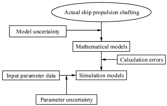
Figure 1.
Sources of uncertainty in mathematical models.
To verify the effectiveness of the method, the responses of the ship propulsion shafting from the test bed are calculated using the established stochastic uncertainty model, and then the dynamic behaviors of shafting with misalignment are investigated. Further, misalignment experiments of the shafting are carried out to verify the correctness of the established model.
2. Establishment Method of Stochastic Uncertainty Model
To better simulate the operation state of the shafting, the shafting misalignment dynamic equation is established, and based on nonparametric theory and stochastic excitation, the stochastic uncertainty model of the ship propulsion shafting is established without considering the scale/size effect. The specific process is as follows.
2.1. Dynamic Equation Under Misalignment
2.1.1. Dynamic Equation
Considering the translation and rotation of the shafting in the X- and Y- directions, the shafting is discretized into several Euler Bernoulli beam elements based on the finite element method. The shafting beam element model is shown in Figure 2.
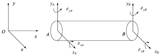
Figure 2.
The shafting beam element model.
As shown in Figure 2, the degrees of freedom of the beam element at the nodes at both ends are represented by vector us as shown in Equation (1).
Considering the influence of the gyroscopic moment of the shafting, the dynamic equation of the shafting beam element can be represented as follows:
where denotes the mass matrix of the beam element, denotes the damping matrix of the beam element, denotes the gyroscopic moment of the beam element, denotes the stiffness matrix of the beam element, and Fe denotes the force vector of the beam element. , , and can be obtained from references [17,18,19], and can be obtained from the proportional damping method [20]. Note that in the following sections, the meaning of the underline of the coefficient matrix means that uncertainty is not considered.
To better simulate the operating state of the shafting system, gravity, unbalanced force, and misalignment force are considered in the force vector. Thus, , where the gravity is , the unbalanced force is and the misalignment force is . The calculation method of the misalignment force will be described in the following subsection. It is worth noting that the unbalanced force and misalignment force only act on a certain node.
The mass matrix of the axial segment beam element comprises a translational inertia matrix and a rotational inertia matrix . Matrices , , , and are represented as follows.
where indicates the mass per unit length, l represents the length of the beam element, r specifies the radius of the beam element, E denotes the elastic modulus, and I signifies the moment of inertia of the cross-section.
Then, the beam elements are assembled, and the dynamic equation of shafting without considering stochastic uncertainty is expressed as follows.
where u denotes the nodal displacement vector of the shafting system, is the mass matrix of the shafting system, is the damping matrix of the shafting system, is the gyroscopic moment of the shafting system, and is the stiffness matrix of the shafting system.
2.1.2. Calculation of Misalignment Force
When the shafting is misaligned, the bearing centerline changes. At this point, the centerline of the shaft system is inclined at an angle α to the centerline (AB) of the rotating shaft of the driving element, as shown in Figure 3.
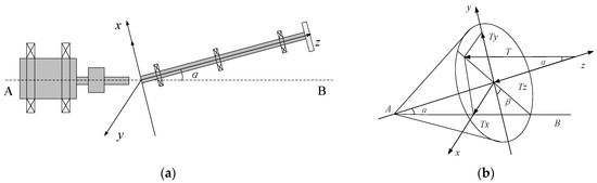
Figure 3.
Shafting system misalignment model: (a) schematic diagram of shafting misalignment; (b) decomposition diagram of misalignment force.
The shafting is driven by a driving moment T. The direction of the driving moment T is horizontal to the left and can be divided into three components Tx, Ty, and Tz, which are expressed as follows.
where Tz drives the shafting along the center of the shafting, and Tx and Ty are perpendicular to the shafting, causing a lateral vibration of the shafting.
According to reference [4], the driving torque can be obtained.
where IR is the polar moment of inertia of the rotor, is the angular velocity of the shaft system, and B2b (b = 1, 2, 3⋯) is a constant independent of the speed. The final shaft element misalignment force can be obtained, as shown in Equation (7).
where F2b = [0,⋯, E2b, G2b]T, ,.
2.2. Introduction of Uncertainties
To better simulate the operating state of the ship propulsion shafting, the shafting data uncertainty and model uncertainty based on nonparametric theory and the stochasticity of the external force of shafting based on stochastic excitation are considered in the misalignment dynamic model established above.
2.2.1. Data Uncertainty and Model Uncertainty
To consider the data uncertainty and model uncertainty of the ship propulsion shafting system, the mass, damping, gyro moment, and stiffness matrix are randomized according to the nonparametric theory [11]. Assuming that A is a symmetric positive definite stochastic matrix of n × n, its probability density function pA must satisfy the following three constraints according to the probabilistic statistical properties of the stochastic matrix proposed by Soize [11].
where is the mathematical expectation of the stochastic matrix A. The domain of integration is the set of all (n × n) real symmetric positive-definite matrices. To ensure that the probability density function of the uncertain stochastic matrix can have practical physical significance, the maximum entropy principle is used to construct the Lagrangian function under the above three basic constraints. The probability density function of the stochastic matrix is obtained by finding the optimal solution.
where cA is a positive constant, and it can be calculated from Equation (10).
where is the Gamma function. The variance of the stochastic matrix A can be expressed as
Because , where is the Frobenius norm, . The divergence parameter is given as Equation (12).
Then, the parameter in Equations (8)–(11) is expressed as Equation (13).
From Equation (13), it can be seen that for an n-dimensional deterministic dynamic system, the larger the value of , the smaller the value of the divergence parameter . When tends to infinity, variances and tend to infinity. At this point, the stochastic matrix A is infinitely close to the average matrix .
The stochastic matrix A can be simulated using the Monte Carlo method by controlling the divergence parameter . For any positive definite symmetric real matrix , it can be decomposed into the product form of a lower triangular matrix and an upper triangular matrix by Cholesky factorization, which is expressed as follows:
where LA is the upper triangular matrix in the real number field. Let , the stochastic matrix A can be further expressed as Equation (15).
where Uj is a vector composed of independent variables that satisfy the standard Gaussian normal distribution.
Thus, multiple samples with stochastic fluctuations within a certain range can be obtained using an average matrix . Therefore, the stochastic mass matrix in the dynamic model of ship propulsion shafting can be obtained, as shown in Equation (16).
The stochastic method for damping matrix Cu and stiffness matrix Ku is the same as that for generating a stochastic mass matrix Mu. However, since the gyroscopic moment is an asymmetric matrix, we use the method in reference [13], as shown below.
where is a stochastic mass matrix, LM+KT is the lower triangular matrix of the Cholesky factor of , H is the lower triangular matrix, and each element in the matrix is statistically independent of the others. The element Hii on the diagonal can be expressed as , where Yii is the gamma distribution with the parameter . Nondiagonal elements are stochastic variables with a standard deviation of a normal distribution.
2.2.2. Excitation Uncertainty
Since the operating environment of ship propulsion shafting is complex, stochastic excitation is introduced to simulate the uncertainty of the external force on the shafting. According to references [21,22,23,24], bounded noise can be used to characterize the stochastic excitation of a system. The bounded noise signal can be assumed as follows:
where Ai is the noise amplitude, Bi(t) is the unit Wiener process, is the random variable uniformly distributed on , is the central frequency, and is the intensity of the stochastic frequency disturbance. The mean value of bounded noise is zero, and its correlation function is expressed in Equation (19).
Its bilateral power spectral density is generated as Equation (20).
According to reference [25], any physically recognizable sample of bounded noise can be approximated by Equation (21).
where is a non-negative stochastic variable independently distributed in the interval , is the random phase uniformly distributed in the interval , N is a sufficiently large positive integer, and is the frequency increment.
Therefore, the stochastic excitation fran is expressed as follows:
where f0 is a constant, and is a stochastic excitation control parameter that can control the size of the stochastic excitation.
Based on the above discussion, the stochastic uncertainty model of ship propulsion shafting can be obtained as follows:
2.2.3. Newmark-β Numerical Solution
The Newmark method excels with its rapid computation speed and unconditional stability, allowing it to closely approximate the exact solutions of dynamic equations. Consequently, this study adopted the Newmark method to address the aforementioned dynamic equations. The core solving principle involves discretizing time and presuming that acceleration adheres to a specific distribution within each time step. By ensuring the time intervals are adequately small and ascertaining the initial velocity and displacement conditions, we can determine the subsequent velocity and displacement, thus enabling the derivation of dynamic responses at a sequence of future time points.
When utilizing the Newmark method for numerical calculations, the system dynamics equations are assumed to have initial conditions set as follows:
If the displacement u(t) and velocity of the system at time t are known, then the acceleration at time t can also be determined. Subsequently, the motion of the system at the next instant will adhere to the following equation.
Assume that the displacement and velocity at time t + Δt adhere to the following relationship:
where β and represent two introduced constant parameters. If , the Newmark method exhibits unconditional stability. By substituting Equations (26) and (27) into the differential equation governing the motion at the subsequent moment, the following equation can be derived:
where , , , , , .
Then, Equations (26) and (27) can be reformulated as follows:
By introducing the equivalent stiffness K* = b1M + b4C + K, the corresponding equivalent external force vector can be expressed as follows:
To summarize, Equation (28) can be derived and presented in the following form:
Given that the displacement, velocity, and acceleration at time t are known, the displacement at time t + Δt can be obtained by solving Equation (32), and then substituting it into Equations (26) and (27) to obtain the velocity and acceleration at time t + Δt.
3. Experimental System for Ship Propulsion Shafting
3.1. Test Bench
A stochastic uncertainty model of the ship propulsion shafting system is established based on the ship shafting system test bench. A schematic of the test bench is presented in Figure 4. A three-phase AC motor with a speed of 0~1000 rpm is connected to the input of the long shaft via coupling to drive the long shaft to rotate. The long shaft is supported by three oil-lubricated journal bearings, which are the intermediate bearing, front stern bearing, and aft stern bearing. The primary parameters are listed in Table 1.
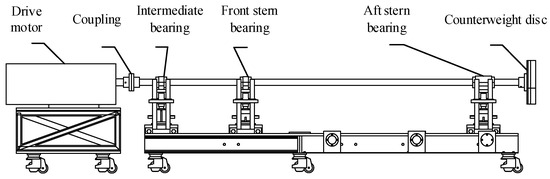
Figure 4.
Schematic diagram of ship propulsion shafting system test bench.

Table 1.
Main parameters of the propulsion shaft system test bench.
3.2. Shafting Model
According to the ship shafting test bench, the shafting is divided into 11 beam elements with a total of 12 nodes, as shown in Figure 5. The beam element between 11 and 12 is a counterweight disc used to simulate the propeller. Nodes 2, 5, and 9 are the positions of the intermediate bearing, front stern bearing, and aft stern bearing, respectively. The radius of the beam elements from number 1 to 10 is 21.5 mm, and that of the number 11 is 58 mm. The lengths of the ship propulsion shafting beam elements are presented in Table 2.
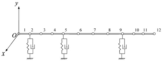
Figure 5.
Ship propulsion shafting model.
Table 2.
Beam elements length parameters of ship propulsion shafting.
4. Numerical and Experimental Investigation on Dynamic Behaviors
4.1. Numerical Study
Based on the stochastic uncertainty model of ship propulsion shafting established above, the dynamic behaviors of ship propulsion shafting with misalignment are analyzed in this section.
4.1.1. Simulation Settings
Misalignment of the shafting can be achieved by adjusting the bearing elevation. In Figure 5, the misalignment force is applied to node 9, the random excitation force is applied to node 10, and the unbalanced force is applied to node 12. The stochastic excitation force is set to be equal in the X- and Y- directions, that is, frx = fry = fran. According to reference [19,26,27], bearing stiffness value is set to 7 × 10⁷ N/m, and bearing damping value is set to 1.5 × 10³ N·s/m. Unless otherwise specified, other parameter settings are shown in Table 3
Table 3.
Parameters used for simulation.
4.1.2. Analysis of Numerical Results
Based on Equations (3) and (22), the dynamic responses of shafting with misalignment under the conditions of certainty and uncertainty can be calculated using the Newmark method [28]. When , the Newmark method exhibits unconditional stability. For the purpose of this study, and β = 0.25 have been chosen for the numerical calculation. Specifically, the dynamics response of interest is located at the stern tube bearing, which corresponds to Node 9 in Figure 4. After the calculations were completed, the results were normalized with the formula Xnorm = 2 (X − Xmin)/(Xmax − Xmin) − 1 to a range of [−1, 1] in order to streamline comparisons, facilitate analyses, and reveal underlying objective patterns. Therefore, the unit of displacement depicted in the subsequent figures is 1, which is typically omitted for simplicity.
Figure 6 shows the dynamic responses calculated for the aft stern bearing without considering the stochastic uncertainty. It can be observed that the time domain signal is a superimposed waveform as shown in Figure 6a. There is an obvious frequency doubling in the frequency spectrum as shown in Figure 6b, and the axis trajectory presents a banana shape as shown in Figure 6c. These dynamic responses indicate that the shafting has the dynamic characteristics of misalignment. Meanwhile, the axis trajectory repeated in a single orbit implies that the dynamic behavior of the shafting is stable.
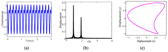
Figure 6.
Dynamic responses calculated for the aft stern bearing under the conditions of certainty: (a) time domain waveform; (b) frequency spectrum; (c) axis trajectory.
To simulate the different levels of stochastic excitation, the stochastic excitation control parameter in Equation (22) is set to 0.2 × 10⁻¹¹, 0.7 × 10⁻¹¹ and 1.2 × 10⁻¹¹, respectively, when the divergence control parameter , and the results of the dynamic response calculated for the aft stern bearing are shown in Figure 7, Figure 8 and Figure 9. Compared with Figure 6, after considering the stochastic uncertainty, it is evident that there are noticeable changes in the shape of the top and bottom peak envelopes, as shown in Figure 7a, Figure 8a, and Figure 9a. Moreover, the frequency spectrum and axis trajectory have changed significantly, i.e., the fractional frequency appears in the spectrum as shown in Figure 7b, Figure 8b, and Figure 9b, and the axis trajectory is a dispersion trajectory of banana shape with a certain width as shown in Figure 7c, Figure 8c, and Figure 9c. Meanwhile, it is worth noting that the axis trajectory becomes increasingly discrete as the stochastic excitation control parameter increases. Therefore, stochastic uncertainty can lead to a change in the dynamic behavior of ship propulsion shafting with misalignment, and it is essential to consider stochastic uncertainty in dynamic research on the misalignment of shafting.
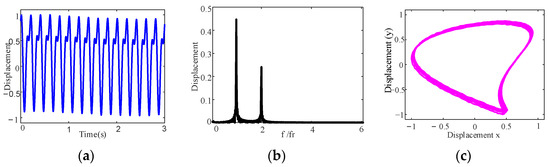
Figure 7.
Dynamic responses of the aft stern bearing under stochastic uncertainty : (a) time domain waveform; (b) frequency spectrum; (c) axis trajectory.
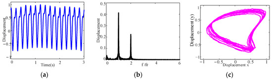
Figure 8.
Dynamic responses of the aft stern bearing under stochastic uncertainty : (a) time domain waveform; (b) frequency spectrum; (c) axis trajectory.
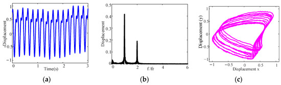
Figure 9.
Dynamic responses of the aft stern bearing under stochastic uncertainty : (a) time domain waveform; (b) frequency spectrum; (c) axis trajectory.
4.2. Experimental Study
To further verify the numerical results, an experimental investigation on the dynamic behaviors of ship propulsion shafting with misalignment under stochastic uncertainty was conducted, and the experimental results were analyzed. It should be noted that the results of the experiments were compared in trend only qualitatively with the results of the numerical simulations.
4.2.1. Experimental Setup
As shown in Figure 10a, the height of each bearing can be adjusted using a worm gear lead screw lifter. The adjustment of the bearing height of the worm gear lead screw lifter is controlled by the hand wheel. The bearing lift is 0.25 mm for each rotation of the handwheel shaft. The accuracy of the height adjustment is 0.05 mm. Two eddy current displacement sensors with a sensitivity of 2500 mv/mm and an effective range of 2 mm are installed on the aft stern bearing pedestal to monitor the bearing height change in real time. Additionally, a counterweight plate with a mass of 20 kg is installed at the output end of the long shaft. In this test, a CZF/BZF eddy current displacement sensor is used to measure the shafting vibration at the aft stern bearing, and its arrangement is shown in Figure 10b.
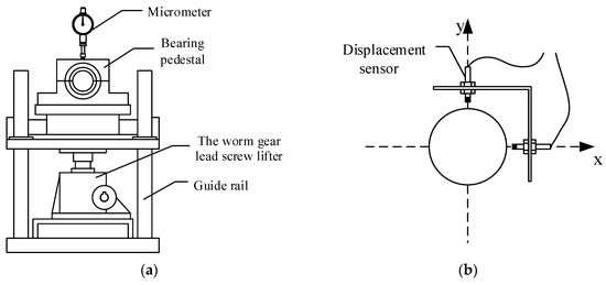
Figure 10.
Key equipment of the shafting test bench: (a) the worm gear lead screw lifter; (b) the schematic diagram of the shafting displacement response measurement.
- Experimental design: To obtain the dynamic behaviors of shafting with misalignment under stochastic uncertainty, the aft stern bearing height is set to 2 mm. Then, the uncertainty caused by hull deformation is determined by adjusting the front stern bearing height. The height fluctuation range of the front stern bearing is set to Δh1 = ±0 mm, Δh2 = ±0.05 mm, Δh3 = ±0.1 mm. Therefore, the above three groups of stochastic uncertainty experiments are conducted on the test bench. The rotating speed is set to 150 rpm, and the running time of each group of experiments is set to 10 min to maintain a stable operation.
- Dynamic response measurements: To measure the dynamic behaviors of the shafting with misalignment in the horizontal (X direction) and vertical (Y direction) directions, two CZF/BZF eddy current displacement sensors are installed near the aft stern bearing as shown in Figure 10. A data acquisition system (model: Ni pxle-1071) is used to collect the displacement signal from the eddy current displacement sensor. The sampling frequency is 1024 Hz, and the sampling time is 120 s.
4.2.2. Analysis of Experimental Results
According to the measured displacement signals in the X and Y directions, the dynamic responses from the aft stern bearing of the shafting, including the time domain waveform, frequency spectrum, and axis trajectory, are obtained under different fluctuation ranges of the front stern bearing height, as shown in Figure 11, Figure 12 and Figure 13.
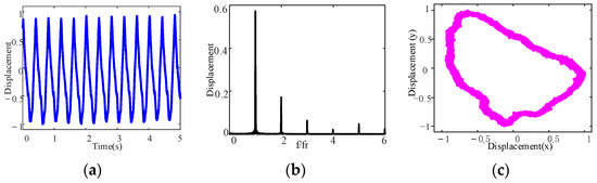
Figure 11.
Dynamic responses from the aft stern bearing under misalignment fluctuation ranges of the front stern bearing height when Δh = 0 mm: (a) time domain waveform; (b) frequency spectrum; (c) axis trajectory.
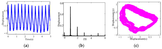
Figure 12.
Dynamic responses from the aft stern bearing under misalignment fluctuation ranges of the front stern bearing height when Δh = ±0.05 mm: (a) time domain waveform; (b) frequency spectrum; (c) axis trajectory.
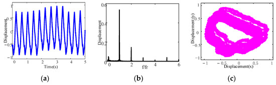
Figure 13.
Dynamic responses from the aft stern bearing under misalignment fluctuation ranges of the front stern bearing height when Δh = ±0.1 mm: (a) time domain waveform; (b) frequency spectrum; (c) axis trajectory.
From Figure 11, Figure 12 and Figure 13, it can be observed that the dynamic responses from the aft stern bearing display are different under different height fluctuation ranges. When Δh = 0 mm, the time domain signal appears as a superimposed waveform, as shown in Figure 11a. In the frequency spectrum, in addition to the first harmonic, there are also the second harmonic and high harmonic, as shown in Figure 11b. The axis trajectory exhibits a banana shape with a small width, as shown in Figure 11c, which indicates that the dispersion degree of the axis trajectory is small, i.e., there are a small number of trajectories deviating from the center of rotation. When Δh = ±0.05 mm, the time domain waveform shows no obvious change, as shown in Figure 12a. There are the first harmonic, second harmonic, high harmonic, and low harmonic in the frequency spectrum, as shown in Figure 12b. The axis trajectory exhibits a banana shape with a large width, as shown in Figure 12c, which indicates that the dispersion of the axis trajectory is large, i.e., there are a large number of trajectories deviating from the center of rotation. When Δh = ±0.10 mm, both the time domain waveform and the frequency spectrum show no obvious change compared with Δh = ±0.05 mm, as shown in Figure 13a,b. The axis trajectory presents a banana shape as well, but the dispersion of the axis trajectory increased significantly, and there are more trajectories deviating from the center of rotation as shown in Figure 13c.
Compared with the dynamic response of numerical calculation in Figure 7, Figure 8 and Figure 9, the dynamic response of the experiment in Figure 11, Figure 12 and Figure 13 has the same trend with the increase in stochastic uncertainty. In addition, the results in Figure 6 are significantly different from those in Figure 11, so the calculation results of the stochastic uncertainty model are closer to the experimental results.
5. Conclusions
To study the dynamic behaviors of propulsion shafting with misalignment under stochastic uncertainty, numerical simulations and experimental verification are performed. In the numerical simulation, the Newmark method is used to solve the dynamic equation of the shafting under stochastic uncertainty. In the experiment, the bearing height is adjusted to create the stochastic uncertainty caused by the hull deformation. Based on the dynamic response obtained by simulation and measurement, the dynamic behaviors of shafting with misalignment under stochastic uncertainty are revealed.
The numerical simulation and experimental results show that the stochastic uncertainty leads to dynamic behavior change in the propulsion shafting with misalignment. When the stochastic uncertainty is small, the displacement response changes slightly, the frequency spectrum shows the first harmonic and second harmonic, and the axis trajectory shows a repetitive trajectory in a narrow area, indicating that the axis system is in a relatively stable state. With the increase in stochastic uncertainty, the displacement response changes significantly, the frequency exhibits an obvious low harmonic, and the axis trajectory is obviously shifted, indicating that the shafting system is operating in an unstable state. Therefore, considering stochastic uncertainty can more accurately simulate and analyze the dynamic behaviors of shafting, thus, effectively guiding the design and installation of shafting, and thus, ensuring the safe navigation of ships.
The nonparametric theory and stochastic excitation simulation method are useful tools for this task. However, there are still challenges in practical applications, such as the quantitative analysis of stochastic uncertainties and their coupling effects. In addition, the influence of scale/size effect on the dynamic response of shafting has not been considered. In the next step, to further study the impact of stochastic uncertainty on ship shafting, quantitative research on stochastic uncertainty will be conducted and the influence of scale/size effect will be considered.
Author Contributions
Conceptualization, P.X., F.Z. and G.L.; methodology, F.Z. and G.L.; software, P.X., F.Z. and X.H.; validation, P.X., F.Z. and G.L.; formal analysis, P.X., F.Z. and X.H; investigation, P.X. and F.Z.; resources, P.X. and F.Z.; data curation, F.Z.; writing—original draft preparation, P.X., F.Z. and G.L.; writing—review and editing, P.X., F.Z. and G.L.; visualization, P.X. and F.Z.; supervision, G.L.; project administration, P.X.; funding acquisition, P.X. and G.L. All authors have read and agreed to the published version of the manuscript.
Funding
This research was funded by the Doctoral Start-up Foundation of Liaoning Province grant number 2024-BS-023; the China Postdoctoral Science Foundation, grant number 2024M750298; the National Natural Science Foundation of China, grant number 52471311; and the Fundamental Research Funds for the Central Universities, grant numbers 3132024215 and 3132023522.
Institutional Review Board Statement
Not applicable.
Informed Consent Statement
Not applicable.
Data Availability Statement
The data presented in this study are available on request from the corresponding author.
Acknowledgments
The authors would like to acknowledge the funders and appreciate each of the anonymous reviewers for their valuable comments and suggestions for improving the quality of this paper.
Conflicts of Interest
The authors declare that they have no known competing financial interests or personal relationships that could have appeared to influence the work reported in this paper.
References
- ABS. Guidance Notes on Propulsion Shafting Alignment; American Bureau of Shipping: Houston, TX, USA, 2019; pp. 11–12.
- Feng, G.Q.; Zhou, B.Z.; Lin, L.J.; Han, Q.K. Transverse vibration measurement and analysis of a three-Point supported dual-span rotor system with angle misaligned flexible coupling. Adv. Mater. Res. 2011, 301, 790–796. [Google Scholar] [CrossRef]
- Jin, Y.; Liu, Z.; Yang, Y.; Li, F.; Chen, Y. Nonlinear vibrations of a dual-rotor-bearing-coupling misalignment system with blade-casing rubbing. J. Sound Vib. 2021, 497, 115948. [Google Scholar] [CrossRef]
- Xu, M.; Marangoni, R. Vibration analysis of a motor-flexible coupling-rotor system subject to misalignment and unbalance-part I: Theoretical model and analysis. J. Sound Vib. 1994, 176, 663–679. [Google Scholar] [CrossRef]
- Saavedra, P.; Ramirez, D. Vibration analysis of rotors for the identification of shaft misalignment-part II: Experimental validation. Proc. Inst. Mech. Eng. Part C J. Mech. Eng. Sci. 2004, 218, 987–999. [Google Scholar] [CrossRef]
- Al-Hussain, K. Dynamic stability of two rigid rotors connected by a flexible coupling with angular misalignment. J. Sound Vib. 2003, 266, 217–234. [Google Scholar] [CrossRef]
- Lees, A. Misalignment in rigidly coupled rotors. J. Sound Vib. 2007, 305, 261–271. [Google Scholar] [CrossRef]
- Fu, C.; Sinou, J.; Zhu, W.; Lu, K.; Yang, Y. A state-of-the-art review on uncertainty analysis of rotor systems. Mech. Syst. Signal Process. 2022, 198, 67–76. [Google Scholar] [CrossRef]
- Hu, X.; Wei, X.; Zhang, H.; Xie, W.; Zhang, Q. Composite anti-disturbance dynamic positioning of vessels with modelling uncertainties and disturbances. Appl. Ocean. Res. 2020, 105, 102404. [Google Scholar] [CrossRef]
- Zhang, Z.; Ma, X.; Hua, H.; Liang, X. Nonlinear stochastic dynamics of a rub-impact rotor system with probabilistic uncertainties. Nonlinear Dyn. 2020, 102, 2229–2246. [Google Scholar] [CrossRef]
- Soize, C. A nonparametric model of random uncertainties for reduced matrix models in structural dynamics. Probabilistic Eng. Mech. 2000, 15, 277–294. [Google Scholar] [CrossRef]
- He, X.; Li, G.; Xing, P.; Lu, L.; Gao, H.; Zhang, H.; Wang, G. Experimental and numerical investigation on dynamic characteristics of ship propulsion shafting under uncertainty based on displacement response. Ocean. Eng. 2021, 237, 0029–8018. [Google Scholar] [CrossRef]
- Murthy, R.; Mignolet, M.; El-Shafei, A. Nonparametric stochastic modeling of uncertainty in rotordynamics-part I: Formulation. J. Eng. Gas Turbines Power 2010, 132, 881–899. [Google Scholar] [CrossRef]
- Murthy, R.; Mignolet, M.; El-Shafei, A. Nonparametric stochastic modeling of uncertainty in rotordynamics-part II: Applications. J. Eng. Gas Turbines Power 2010, 132, 92502. [Google Scholar] [CrossRef]
- Papanikolaou, A.; Mohammed, E.; Hirdaris, S. Stochastic uncertainty modelling for ship design loads and operational guidance. Ocean. Eng. 2014, 86, 47–57. [Google Scholar] [CrossRef]
- Guedes Soares, C. Effect of spectral shape uncertainty in the short term wave-induced ship responses. Appl. Ocean. Res. 1990, 12, 54–69. [Google Scholar] [CrossRef]
- Nelson, H.; Mcvaugh, J. The dynamics of rotor-bearing systems using finite elements. Trans. Am. Soc. Mech. Eng. J. Eng. Ind. 1976, 98, 593–600. [Google Scholar] [CrossRef]
- Nelson, H.; Meacham, W.; Fleming, D.; Kascak, A.F. Nonlinear analysis of rotor-bearing systems using component mode synthesis. J. Mech. Des. 1983, 102, 352–359. [Google Scholar] [CrossRef]
- Han, Q.; Zhang, Z.; Wen, B. Periodic motions of a dual-disc rotor system with rub-impact at fixed limiter. Proc. Inst. Mech. Eng. Part C J. Mech. Eng. Sci. 2008, 222, 1935–1946. [Google Scholar] [CrossRef]
- Volpi, L.; Ritto, T. Probabilistic model for non-proportional damping in structural dynamics. J. Sound Vib. 2021, 506, 116145. [Google Scholar] [CrossRef]
- Huang, W.; Gan, C. Bifurcation analysis and vibration signal identification for a motorized spindle with random uncertainty. Int. J. Bifurc. Chaos 2019, 29, 1950001. [Google Scholar] [CrossRef]
- Taflanidis, A.; Vetter, C.; Loukogeorgaki, E. Impact of modeling and excitation uncertainties on operational and structural reliability of tension leg platforms. Appl. Ocean. Res. 2013, 43, 131–147. [Google Scholar] [CrossRef]
- Gan, C.; Guo, S.; Lei, H.; Yang, S.-X. Random uncertainty modeling and vibration analysis of a straight pipe conveying fluid. Nonlinear Dyn. 2014, 77, 503–519. [Google Scholar] [CrossRef]
- Deng, J.; Xie, W.; Pandey, M. Stochastic stability of a fractional viscoelastic column under bounded noise excitation. J. Sound Vib. 2014, 333, 1629–1643. [Google Scholar] [CrossRef]
- Shinozuka, M.; Janc, M. Digital simulation of random processes and its applications. J. Sound Vib. 1972, 25, 111–128. [Google Scholar] [CrossRef]
- Liu, Y.; Dou, J.; Wen, B. Identification technique of misalignment-rubbing coupling fault in dual-disk rotor system supported by rolling bearing. J. Vibro Eng. 2015, 17, 287–299. [Google Scholar]
- Han, Q.; Yao, H.; Wen, B. Parameter identifications for a rotor system based on its finite element model and with varying speeds. Acta Mech. Sin. 2010, 26, 299–303. [Google Scholar] [CrossRef]
- Filippi, M.; Carrera, E. Stability and transient analyses of asymmetric rotors on anisotropic supports. J. Sound Vib. 2021, 500, 116006. [Google Scholar] [CrossRef]
Disclaimer/Publisher’s Note: The statements, opinions and data contained in all publications are solely those of the individual author(s) and contributor(s) and not of MDPI and/or the editor(s). MDPI and/or the editor(s) disclaim responsibility for any injury to people or property resulting from any ideas, methods, instructions or products referred to in the content. |
© 2024 by the authors. Licensee MDPI, Basel, Switzerland. This article is an open access article distributed under the terms and conditions of the Creative Commons Attribution (CC BY) license (https://creativecommons.org/licenses/by/4.0/).