TG-PGAT: An AIS Data-Driven Dynamic Spatiotemporal Prediction Model for Ship Traffic Flow in the Port

Abstract

Accurate prediction of ship traffic flow is essential for developing intelligent maritime transportation systems. To address the complexity of ship traffic flow data in the port and the challenges of capturing its dynamic spatiotemporal dependencies, a dynamic spatiotemporal model called Temporal convolutional network-bidirectional Gated recurrent unit-Pearson correlation coefficient-Graph Attention Network (TG-PGAT) is proposed for predicting traffic flow in port waters. This model extracts spatial features of traffic flow by combining the adjacency matrix and spatial dynamic coefficient correlation matrix within the Graph Attention Network (GAT) and captures temporal features through the concatenation of the Temporal Convolutional Network (TCN) and Bidirectional Gated Recurrent Unit (BiGRU). The proposed TG-PGAT model demonstrates higher prediction accuracy and stability than other classic traffic flow prediction methods. The experimental results from multiple angles, such as ablation experiments and robustness tests, further validate the critical role and strong noise resistance of different modules in the TG-PGAT model. The experimental results of visualization demonstrate that this model not only exhibits significant predictive advantages in densely trafficked areas of the port but also outperforms other models in surrounding areas with sparse traffic flow data.

1. Introduction

Predicting ship traffic flow is essential for optimizing ship traffic organization within the port [1]. Accurate traffic prediction results not only facilitate ship route planning at the micro level but also contribute to the enhancement of efficient navigation management for regional traffic from a macro perspective. Ports are hubs for ship entry and exit operations and key nodes in international logistics. Predicting ship traffic flow in port waters can enhance navigation efficiency and provide necessary data and information to support the planning and construction of smart waterways and ports.

Traffic flow prediction is the foundation of intelligent transportation systems and has become a research focus for scholars at home and abroad. Significant advancements have been achieved across various fields and scenarios within transportation [2,3,4,5]. In the early stages, due to limitations in the collection of maritime traffic data, ship traffic flow prediction primarily relied on classical time-series statistical models or their improved and combined versions, such as Autoregressive Integrated Moving Average (ARIMA) [6], Bayesian Estimation [7], and Kalman Filtering (KF) [1]. Time-series statistical models can yield reliable predictions for stable traffic flow. However, they exhibit significant errors when addressing complex, dynamic, nonlinear, and nonstationary maritime traffic prediction challenges, failing to meet the practical requirements of engineering applications.

Subsequently, machine learning has consistently demonstrated exceptional performance in addressing complex scenario problems, and the methods have been extensively applied to traffic flow prediction. Compared to time-series statistical models, machine learning models, such as Neural Networks [8], K-Nearest Neighbors (KNN) [9], Matrix Factorization [10], and Support Vector Machine (SVM) [11], are more effective in addressing the issue of low prediction accuracy in traffic flow prediction due to nonlinearity, nonstationarity, and other characteristics. More scholars have adopted combining or improving models to better handle the uncertainty of a single machine learning model, ultimately improving prediction accuracy and robustness. Han et al. [12] proposed a Fractional Order Gradient Descent with a Momentum method for updating the weights of the Radial Basis Function neural network (FOGDMRBF) to mitigate the oscillation phenomenon during the training of the Radial Basis Function neural network (RBF). Zhao et al. [13] employed video image extraction technology in conjunction with machine learning algorithms to accurately predict ship traffic flow speed. Chen et al. [14] proposed a method for predicting ship traffic flow by applying the whale optimization algorithm to an extreme learning machine and utilizing it for predicting ship traffic congestion.

With the advancement of technologies such as artificial intelligence and AIS, the collection of extensive ship traffic flow data has propelled the development and research of big data-driven predictive models. Traditional machine learning methods have limited capability to uncover profound and implicit spatiotemporal correlations within big data, thereby driving the gradual adoption of deep learning in ship traffic flow prediction. The fundamental deep learning methods mainly include Convolutional Neural Networks (CNNs) [15], Recurrent Neural Networks (RNNs) [16], and Long Short-Term Memory (LSTM) [17]. These methods can automatically extract temporal or spatial features from historical traffic data, thereby enabling the establishment of more accurate prediction models. Ship traffic flow has obvious spatiotemporal dependence. Scholars have integrated the features of deep learning architectures to enhance the utilization of spatiotemporal feature extraction advantages from various methods through the combination of models or the incorporation of components, including attention mechanisms, gated recurrent units, and linear superposition units. Xu and Zhang [18] developed a Gated Recurrent Unit (GRU) model based on RNN to accurately predict and analyze the spatiotemporal variation features of ship traffic flow near offshore wind farms. Li et al. [19] proposed an Improved CNN-LSTM Network with a Similarity Grouping (ICLSGNet) that integrates CNN, LSTM, and similarity grouping to effectively extract the spatiotemporal attributes of traffic flow data and the similarity features of neighboring target areas, thereby achieving accurate predictions of ship traffic flow in Chengshantou traffic separation waters. EI et al. [20] developed a speed prediction model for ships in the Vessel Traffic Service (VTS) area by integrating the Transformer attention mechanism into the RNN model, providing a reference for ship speed supervision in the VTS area. Ding et al. [21] constructed a CNN-LSTM prediction model for ship traffic flow and optimized its hyperparameters using the Gorilla Troop Optimizer (GTO), enhancing prediction accuracy. Ma et al. [22] integrated Seasonal and Trend decomposition using Loess (STL) and Multi-head Self-Attention (MSA) into an LSTM network to accurately predict the arrival time intervals of ships in the waterway.

In order to enhance the learning and training efficiency of prediction models and explore the spatiotemporal global features of ship traffic flow, prediction models based on Graph Neural Network (GNN) have been developed, establishing themselves as a mainstream direction in the field of traffic flow prediction. Li et al. [23] developed a novel fine-grained spatiotemporal graph network model based on AIS, Lloyd’s Register ship records, and port geographic spatial data, achieving traffic flow predictions for multiple ports, including Rotterdam, Shanghai, and Hong Kong. Li et al. [24] designed a Semi-Dynamic Spatial Graph network (SDSG) module that integrates LSTM and transformer temporal feature extraction components to capture spatial features and predict the traffic status of waterways. Man et al. [25] proposed a combined model that integrates GAT and LSTM to predict traffic flow in the Yangtze River inland waterway, achieving satisfactory prediction results.

GNN plays a crucial role in capturing and accurately predicting the spatiotemporal relationships of traffic flow. However, ship traffic flow in the port not only exhibits temporal autocorrelation and spatial dependence but is also influenced by periodic dynamic natural factors, such as tidal changes, presenting complex spatiotemporal dynamic features. Furthermore, the complexity of the port navigation environment, the diversity of functional water areas, and the significant differences in factors, such as ship type parameters, navigation rules, and channel water depth, all greatly impact ship traffic flow in the port. It is crucial to extract the spatiotemporal dependencies of varying durations in ship traffic flow data and identify the dynamic features for accurate prediction of ship traffic flow in port waters.

To solve the problems in predicting ship traffic flow in the port mentioned above, this paper develops a multidimensional spatiotemporal feature fusion model, TG-PGAT, that explores the spatiotemporal dependencies of ship traffic flow from local and global perspectives. Firstly, the model decomposes the historical sequence of ship traffic flow and extracts multiple traffic flow sequence features. Furthermore, the TCN and BiGRU models extract time-related information from multi-feature traffic flow at various intervals. Meanwhile, the global correlation coefficient matrix P of ship traffic flow space in port waters is calculated using the Pearson Correlation Coefficient (PCC) and fused with the ship traffic flow matrix to obtain the local dynamic spatial features of the port through GAT. The main contributions of this paper are as follows:

• Aiming at the cyclical patterns and dynamic spatiotemporal dependence features of ship traffic flow in the port, a multidimensional spatiotemporal feature fusion model is constructed to tap the spatiotemporal dynamic influence and interdependence of ship traffic flow. The model can accurately capture the spatiotemporal dependencies of different nodes in the port, enabling precise predictions of traffic flow with significant spatiotemporal changes in complex navigational environments.
• The TCN and BiGRU models are employed to extract temporal features from ship traffic flow, significantly enhancing the performance of the model in the time learning module. Based on GAT, spatial features in ship traffic flow are extracted by utilizing the spatial correlation coefficient matrix and traffic flow matrix, enhancing the model’s capability to model node relationships and features.
• Based on the historical AIS data from the port, the performance of the constructed model is evaluated comparatively. The results show that the TG-PGAT model has higher accuracy, robustness, and anti-interference capability, enabling the prediction and analysis of ship traffic flow dynamics in the port.

The rest of the paper is as follows: Section 2 describes the problem of ship traffic flow in the port and details the construction process of the TG-PGAT model; Section 3 conducts experimental evaluation and comparative analysis of the model’s performance; and Section 4 presents the conclusions of the research.

2. Materials and Methods

2.1. Problem Description

2.1.1. Construction of Ship Traffic Map in the Port

This paper investigates the traffic flow in port waters, with a specific focus on Qingdao Port as the case study. Qingdao Port is located in the central region of the Yellow Sea, adjacent to Japan and South Korea to the east. It has nearly 40 major and minor shipping routes, and the tidal patterns in the waters of Qingdao Port are significant. There are many ultra-large ships, such as oil tankers, container ships, and bulk carriers, coupled with many fishing boats and frequent sea fog, significantly impacting the traffic flow and navigation safety of ships in Qingdao Port. Therefore, it is necessary and representative to take ship traffic flow in Qingdao Port as the research object.

Considering the scope of the studied waters and the typical scale of the port functional waters, the entire study area is divided into square grids with a side length of one nautical mile, totaling 9 × 17 grids. For the identification of each grid, each grid, i, is labeled by locating it in the order of the coordinate axes (x1y1~x17y9). The gridding of Qingdao Port waters is shown in Figure 1 (35.96° N–36.10° N, 120.18° E–120.50° E).

The partitioned port ship traffic grid is represented as a graph G = (N, E, A), where grid i is a node N_i in the graph, E is a set of edges for connectivity between nodes, and $A\in {\mathit{R}}^{N\times N}$ denotes the adjacency matrix of the ship traffic graph G. Historical data of ship traffic flow can be represented on the traffic network as a time series X = (X¹, X², …, X_i^t,…, X^t), where $X_i^t\in {\mathit{R}}^{N\times d}$ represents the traffic flow information of node i of the ship traffic graph G at time step t, and d is the dimension of the traffic flow eigenvalue (traffic flow volume, traffic flow density, traffic flow speed). Then, the problem of predicting ship traffic flow in the port can be defined as the following Equation (1):

$$T_i^t=f(G,X_i^t)$$

(1)

In Equation (1), $T_i^t$ represents the traffic flow information of node i predicted by the model over the duration t, and G represents the topological structure relationship of distributed nodes.

2.1.2. Analysis of Spatiotemporal Features of Ship Traffic Flow in the Port

As shown in Figure 2, the ship flow data within each grid area are influenced by both time and space. For instance, the ship traffic flow data at the predicted moment of grid x5y5 are affected by both current and historical traffic flow variations, as well as by the correlation of adjacent waters such as grids x4y4, x5y4, x6y5, and x4y5.

Meanwhile, the navigation situation in port waters is more complex than in other waters. The influencing factors include stable surrounding waterways, anchorages, and berths, as well as the cyclical patterns of ships entering and leaving the port under tidal effects. These influencing factors cause the spatiotemporal correlation of traffic flow between each grid to change dynamically over time, with obvious temporal correlation, periodicity, and instability. Therefore, relying solely on the adjacency matrix within the graph network is insufficient for effectively extracting the spatiotemporal correlation between nodes [22].

• Temporal Feature Analysis

In order to better clarify the temporal features of ship traffic flow in the port, the traffic flow data of some areas in Figure 2 were randomly selected over a period of 30 consecutive days, with a time interval of 1 h, and decomposed using the Variational Mode Decomposition (VMD) method [26]. The results are shown in Figure 3.

In Figure 3, the horizontal axis represents the time point for collecting ship traffic flow, while the vertical axis indicates the values of ship traffic flow. This depiction reflects the fluctuations and changes in ship traffic flow over various durations. As illustrated in Figure 3, the original sequence data of ship traffic flow in the port exhibit significant nonlinear and nonstationary characteristics. After VMD decomposition, each component has its own fixed pattern, representing traffic flow data components at different time scales. The smaller frequencies (IMF1, IMF2, IMF3) have smaller fluctuations, reflecting the periodic trends of ship traffic flow in the port and representing the more stable parts of components. The higher frequencies (IMF4, IMF5) reflect the volatility of ship traffic flow in the port over varying durations, and the oscillation patterns in adjacent durations are relatively similar, with a certain correlation.

The results of the VMD time-series decomposition of ship traffic flow in the port better reflect that ship traffic flow is affected by temporal proximity and cyclical patterns caused by tidal changes. It also reflects the long-term trend presented by the inherent characteristics of the shipping industry. The implied characteristics of proximity, periodicity, and trend in the time series of ship traffic flow in the port are fully reflected.

• Spatial Feature Analysis

In order to extract the spatial correlation of ship traffic flow in the port among different nodes, PCC [27] is employed for analysis, as shown in Equation (2):

$$P_{x,y}={\displaystyle \frac{\mathrm{cov}(x,y)}{\sigma x\sigma y}}$$

(2)

In Equation (2), cov(x,y) denotes the covariance of variables x and y, while σx and σy denote the standard deviation of the two variables, respectively. The value of P_x,y ranges from [−1,1], reflecting the degree of linear correlation between the two variables, with larger values indicating a stronger correlation. Eight adjacent grid nodes (within the yellow line box in Figure 2) are randomly selected from the network map of ship traffic flow in the port. The correlation magnitude of each grid node in space is calculated using Equation (2) to extract the correlation of ship traffic flow in the port at different grid nodes. The correlation results are shown in Figure 4.

The thermal values of different colors in Figure 4 demonstrate the degree of influence on the spatial relationship of traffic flow between adjacent nodes. The traffic flow correlation coefficients between nodes vary widely due to the influence of various functional areas such as waterways, anchorages, berths, and other navigational regulations in port waters. Some grid nodes, such as x4y4, x4y5, and x5y5, are located in the critical intersection areas near the port entrance. Due to the criticality of their location, these nodes exhibit significant correlations not only with adjacent nodes but also with nonadjacent nodes. Therefore, a global spatial correlation coefficient matrix P of ship traffic flow in the port can be constructed using PCC. This helps to uncover better the hidden spatial relationships and potential features of ship traffic flow in the port, thereby improving the accuracy of traffic flow predictions.

2.2. Model Construction

Based on analyzing the spatiotemporal features of ship traffic flow in the port, the TG-PGAT model is proposed to address the complexity of ship traffic flow and the limitations of existing traffic flow prediction methods. The model employs historical data of ship traffic flow in the port as input. The input data are processed using VMD decomposition and fed into TCN and BiGRU models to construct the temporal feature extraction module designed to extract local and global traffic flow temporal features. Meanwhile, the extraction of spatial features is facilitated by the node correlation matrix P, which is determined by PCC and GAT. Finally, a dual-layer multilayer perceptron is used for the fusion of multidimensional temporal and spatial features, while a Fully Connected Layer (FC Layer) module is employed for feature mapping to output the final prediction results. The model architecture is shown in Figure 5.

2.2.1. Model Input

In order to reduce the complexity of ship traffic flow data and minimize the impact of randomness, nonlinearity, and other factors on the prediction results of the original traffic flow data, the VMD method is first employed to decompose the ship traffic flow data. The VMD method effectively mitigates the nonstationarity of time series characterized by high complexity and pronounced nonlinearity. It has been maturely applied and achieved good results in data processing across multiple research directions, such as ship traffic flow prediction [14,28,29], significantly enhancing predictive accuracy. The equations associated with the VMD method are not detailed here.

After the VMD decomposition of ship traffic flow data, K IMF feature sequences are obtained. These sequences are then input into the temporal and spatial feature modules to extract spatiotemporal characteristics pertinent to future traffic flow.

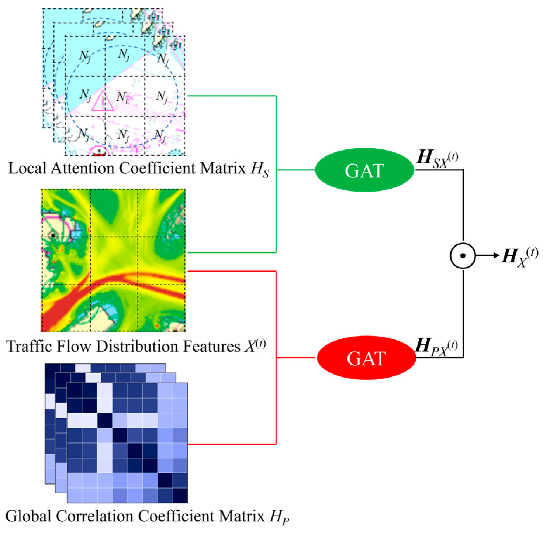
2.2.2. Spatial Feature Extraction Module

GAT is a mainstream method widely used to capture the spatial correlation of traffic flow in current traffic flow prediction problems, which can effectively extract the dynamic relationships between nodes and edges of graph networks [30]. To effectively extract the spatial features of ship traffic flow in the port, the attention matrix between neighboring nodes of the ship traffic flow graph is first computed using GAT, while simultaneous analysis is carried out by combining the correlation features between nodes.

• The Calculation of Spatial Attention Coefficient of Ship Traffic Flow in the Port

The core process of GAT computation involves dynamically assigning weights to different vertices at distinct time steps, as illustrated in Figure 6. Firstly, the spatial attention coefficient $e_{ij}^{(t)}$ is computed between the central node N_i and all nodes N_j in its neighborhood. Then, it is normalized using the softmax operation. Finally, the obtained normalized attention coefficient ${\alpha }_{ij}^{(t)}$ is aggregated as weights for weighted summation.

The specific calculation of the attention coefficient after normalization can be expressed by Equation (3):

$${\alpha }_{ij}^{(t)}=softmax(e_{ij}^{(t)})={\displaystyle \frac{\exp (e_{ij}^{(t)})}{{\displaystyle {\sum }_{N_k\in Ne(N_i)}{e}_{ik}^{(t)}}}}$$

(3)

In Equation (3), $e_{ij}^{(t)}$ denotes the importance of node N_j to node N_i at time t, and Ne(i) represents the neighborhood of node N_i. In predicting traffic flow in the port, as depicted in Figure 1, each node needs to consider the influence of neighboring nodes on its traffic flow. Equation (3) facilitates a more precise allocation of attention weights to each node, thereby enabling the comparability of weights among different nodes.

Then, Equation (4) can be employed for aggregation to obtain the new eigenvector value $x_i^{(t{)}^{\prime }}$ of the central node N_i:

$$x_i^{(t{)}^{\prime }}=f({\displaystyle {\sum }_{N_j\in Ne(N_i)}{\alpha }_{ij}^{(t)}}{W}_{x_{ij}}^{(t)})$$

(4)

In Equation (4), f(.) represents a nonlinear activation function employed to regulate the output range of new eigenvector values. After obtaining the attention weights that capture the mutual influence between nodes using Equation (3), the traffic flow of each neighboring node is multiplied by its attention weight with respect to the current node. By performing a weighted summation, the node’s feature vector $x_i^{(t{)}^{\prime }}$ can be obtained.

The impact of traffic flow in port waters must not only account for the relevant effects between adjacent nodes but also for multiple factors such as node distance and the influence of different spatial regions (referred to as multi-head attention). To ensure the stability of the learning process of GAT, the spatial attention mechanism is extended to a multi-head attention mechanism. The outputs from each attention head are subsequently fused to enhance the accuracy of local spatial feature predictions for traffic flow. The fusion process is shown in Equation (5) below:

$$x_i^{(t{)}^{\prime }}=W_o\left[{\parallel }_{j=1}^M{x}_i^{(t_j{)}^{\prime }}\right]$$

(5)

In Equation (5), M is the number of independent attention heads with respective parameters, representing the number of spatial factors within the port waters that may influence the traffic flow, such as adjacent areas, anchorages, channels, and berths. $x_i^{(t_j{)}^{\prime }}$ is the output eigenvector of the j-th attention head at time t, W_o is the corresponding learning parameter, and $\parallel$ denotes the splicing operation.

• Node Correlation Calculation of Ship Traffic Flow in the Port

The spatial feature analysis of ship traffic flow distribution in the port, as presented in Section 2.1.2, indicates that, due to the diverse functional distribution in the port, relying solely on the proximity matrix of GAT is inadequate for accurately determining the spatial relationships between nodes. Therefore, employing PCC to calculate the correlation between nodes can more accurately uncover the hidden associations between ship traffic flow nodes in port waters, facilitating the extraction of global node correlation features. The specific calculation is shown in Equation (6):

$$P_{x,y}={\displaystyle \frac{{\displaystyle \sum _{i=1}^T(x_i-\overline{x})(y_i-\overline{y})}}{\sqrt{{\displaystyle \sum _{i=1}^T{(x_i-\overline{x})}^2}}\sqrt{{\displaystyle \sum _{i=1}^T{(y_i-\overline{y})}^2}}}}$$

(6)

In Equation (6), P_x,y represents the correlation value between different nodes of the graph network, T is the length of the traffic flow time series, x_i and y_i, respectively, represent the values of the traffic flow time series x and y at time i, while $\overline{x}$ and $\overline{y}$ denote their respective averages.

• Fusion of Local Spatial Attention Features and Global Node Correlation Features

To enhance the capability of the ship traffic flow prediction model in capturing spatial features in the port, the extracted spatial attention local features are fused with the global correlation features. The specific feature fusion strategy is shown in Figure 7.

As shown in Figure 7, firstly, GAT is employed to model the nodes and their adjacent nodes of the port transportation network. This approach adaptively learns the attention weights between nodes, captures spatial local dynamic features, and derives the spatial local attention feature matrix H_SX^(t) of ship traffic flow in the port by convolving the spatial attention coefficient matrix H_S with the traffic flow distribution matrix X^(t). Secondly, the PCC coefficient H_P between the calculated nodes is nonlinearly operated with the traffic flow distribution matrix X^(t) to construct the spatial global correlation feature matrix H_PX^(t). Thirdly, H_SX^(t) and H_PX^(t) are processed in parallel, and the Hadamard product $\odot$ is used to perform element-level matrix multiplication on these two features. The nonlinear transformation is conducted using the Rectified Linear Unit (ReLU) activation function to better extract the spatial interaction features of ship traffic flow in the port. Finally, the fused feature representation H_X^(t) is obtained, as shown in Equation (7):

$$H_{X^{(t)}}=\mathrm{Re}LU(H_{S{X}^{(t)}}\odot H_{P{X}^{(t)}})$$

(7)

2.2.3. Temporal Feature Extraction Module

This module is divided into two components: local time-series feature extraction and global time-domain feature extraction, based on the periodicity, nonlinearity, and instability of the ship traffic flow time series in the port. It adopts the fusion of two branches of TCN and BiGRU models, leveraging the strengths of each model to extract both local and global temporal features of ship traffic flow.

• Local Time-series Feature Extraction of Ship Traffic Flow in the Port

The TCN model is a temporal convolutional network for solving sequence modeling problems under causal constraints. This concept was first introduced in 2016 [31]. And it was empirically evaluated in 2018 [32], demonstrating that the TCN model can efficiently address long-distance dependency problems of time-series data and has computational efficiency advantages compared to RNN and LSTM. It is extensively utilized in traffic flow prediction across various domains [33,34,35,36]. The architecture of the TCN model is shown in Figure 8.

As shown in Figure 8, the feature extraction model of the ship traffic flow sequence in the port is divided into three parts: a, b, and c. Among these components, a represents the architecture of the TCN model’s operational process, which includes the stacking of L layers of residual blocks b and the final output layer. This structure extracts abstract features from the time-series data of ship traffic flow in the port, layer by layer. b is the residual block of the TCN model, consisting of two layers of dilated causal convolution and nonlinear layers. It captures long-term dependencies in the sequence through residual connections. c is the main structure expansion causal convolution part of the TCN model. It adjusts the size of the sensory field by changing the expansion coefficient d, enabling the network to flexibly adapt and output the quantity of received historical information. The expression for the expansion convolution operation is

$$F(t)=(X_d^{*}f)(t)={\displaystyle \sum _{i=0}^{k-1}f(i)\cdot }{X}_{t-d_i}$$

(8)

Equation (8) defines the operation of the dilated convolution F on an element t of a one-dimensional sequence $x\in {\mathbb{R}}^n$ with respect to a filter r f:{0, 1,…, k − 1}→ℝ, where k is the filter size, d is the expansion coefficient, and * is the convolution operation. From F(t), it is evident that the size of the receptive field of the output sequence in the inflated causal convolution c is adjusted by k and d and is only affected by the previous historical data. This property can be effectively leveraged to extract the local time-series feature $T_{L{X}^{(t)}}$ of ship traffic flow in the sequence.

• Global Time-domain Feature Extraction of Ship Traffic Flow in the Port

By analyzing the temporal features of ship traffic flow in the port, it can be concluded that the traffic flow in a certain grid is not only related to historical traffic flow but also influenced by future traffic flow states. Using BiGRU [37,38] can effectively extract global features and dynamic changes in the traffic flow sequence from both forward and backward temporal directions. At the same time, considering the similarity of features between historical and future moments of ship traffic flow, the self-attention mechanism is further integrated to analyze the temporal features extracted by BiGRU. This enables the model to focus more specifically on important temporal features, enhancing its capability to perceive and generalize across multi-feature temporal sequences. The extraction steps are shown in Figure 9 below:

As shown in Figure 9, firstly, the traffic flow time-series feature H_K^(t), decomposed by VMD, is utilized as the input of BiGRU. The forward output feature ${\overrightarrow{\mathit{H}}}^{(t)}$ of GRU can be obtained by solving the forward equation. The specific calculation process is as follows:

$$\begin{gathered} {\mathcal{Z}}^{\left(t\right)}=\sigma \left(W_{Ɀ}\right[H^{\left(t-1\right)},H_{K^{\left(t\right)}}\left]\right) \\ {r}^{(t)}=\sigma (W_r[H^{(t-1)},H_K^{(t)}]), \\ {\tilde{H}}^{(\mathrm{t})}=tanh(W_H[r^{(t)}\odot H^{(t-1)},H_K^{(t)}), \\ {\overrightarrow{H}}^{\left(t\right)}=\left(1-{\mathcal{Z}}^{\left(t\right)}\right) ⨀ H^{\left(t-1\right)}+{\mathcal{z}}^{\left(t\right)} ⨀ {\tilde{H}}^{(t-1)} \end{gathered}$$

(9)

In Equation (9), ${\mathcal{z}}^{\left(t\right)}$, $r^{\left(t\right)}$ is the update gate introduced in GRU, determining the amount of information from the previous time step’s hidden state H^(t−1) and the current time step’s input H_K^(t) (the traffic flow features at the current time point) that needs to be retained in the hidden state H^t at the current time step. r^(t) is a reset gate introduced in GRU, which determines the amount of information that needs to be forgotten in the hidden state H^(t−1) at the previous time step to calculate the candidate hidden state ${\tilde{H}}^{(t)}$ output at the current time. ${\tilde{H}}^{(t)}$ combines the traffic flow feature H_K^(t) at the current time point with the historical traffic flow information processed by the reset gate. ${\overrightarrow{\mathit{H}}}^{(t)}$ is the final prediction of traffic flow at the current time point, and ⊙ is the Hadamard product.

Similarly, the backward calculation of the next layer GRU can also yield backward output features. Then, the BiGRU model can output the traffic flow time-domain feature ${\widehat{H}}^{(t)}$.

Secondly, to clarify the importance of the input features of ship traffic flow at various times, a self-attention mechanism is introduced into the BiGRU model. This mechanism aims to better explore the important time-domain features of traffic flow, thereby improving the accuracy of the model. The scoring process of the self-attention mechanism is shown in Equation (10) below:

$$\begin{array}{l}{\epsilon }^{(t)}=tanh(W_w{\widehat{H}}^{(t)}+b_w),\\ {\alpha }^{(t)}={\displaystyle \frac{exp(u_w^T{\epsilon }^{(t)})}{{\displaystyle {\sum }_t(exp(u_w^T{\epsilon }^{(t)}))}}},\\ H^{(t)}={\displaystyle {\sum }_t{\alpha }^{(t)}}{\widehat{H}}^{(t)}.\end{array}$$

(10)

In Equation (10), u_w corresponds to Query in the self-attention mechanism, used to inquire about the time points in the traffic flow sequence that are most relevant to the traffic volume at the current time point. ε^(t) corresponds to Key in the self-attention mechanism, representing the attention score obtained from the output feature ${\widehat{H}}^{(t)}$ in the BiGRU model at time t, reflecting the importance of traffic flow information at this time point to the current prediction. The output feature corresponds to Value in the self-attention mechanism. α^(t) represents the attention weight coefficients corresponding to ${\widehat{H}}^{(t)}$ at different time points, indicating the importance of each time point relative to other time points at all time points. W_w, b_w, and u_w are set parameters. H^(t) is the weighted sum of the hidden states at all time points and their corresponding attention weights, capturing the most important information in the global traffic flow time-domain sequence. The global time-domain feature $T_{G{X}^{(t)}}$ of traffic flow is obtained by weight allocation through the self-attention mechanism.

Finally, the local time-series feature $T_{L{X}^{(t)}}$ and the global time-domain feature $T_{G{X}^{(t)}}$ of ship traffic flow in the port are fused in series to effectively preserve the original traffic flow feature information. The tandem operation process is shown in Equation (11) below:

$$T_{X^{(t)}}=T_{L{X}^{(t)}}\oplus T_{G{X}^{(t)}}$$

(11)

In Equation (11), $\oplus$ is the tandem operation, and $T_{X^{(t)}}$ is the temporal feature of ship traffic flow in the port extracted and fused using two branches of TCN and BiGRU models.

2.2.4. Feature Fusion Module

After processing the spatial and temporal feature extraction modules, the spatiotemporal features of ship traffic flow in the port are obtained. Here, a dual-layer multilayer perceptron is employed for feature fusion, integrating the spatial and temporal features into a single eigenvector Y to better handle the spatiotemporal nonlinear features of ship traffic flow in the port. The FC Layer is a regression layer for prediction, outputting the predicted traffic flow feature sequence $\widehat{Y}$. The expression for Feature Fusion Layer (FF Layer) is shown in Equation (12) below:

$$Y=F{C}^2(F{C}^1(H_{X^{(t)}}\parallel T_{X^{(t)}})$$

(12)

3. Experiment

3.1. Experimental Data

Based on the selection of the study port and the definition of the water area scope in Section 2.1, the ship AIS data for September 2022 within the water area were extracted from the authorized Hifleet database (www.hifleet.com) as the experimental dataset. Given that the prediction model relies on time-series data for predictive mining, it is necessary to screen and process the ship traffic flow in the port from a temporal perspective. Firstly, the ship AIS data collected within the study waters range were processed, such as cleaning and interpolation. To address the data noise issue in ship AIS data, the Density-Based Spatial Clustering of Applications with Noise (DBSCAN) clustering method is used to identify and process noisy trajectories. Additionally, the mean interpolation method is employed to clean and interpolate noisy data, ensuring the structural integrity of the data. To address the issue of decreased data quality caused by missing ship trajectory data in AIS data, the Bidirectional Long Short-Term Memory (Bi-LSTM) algorithm is used to interpolate and reconstruct the identified missing segments of trajectory data. The total number of raw AIS data within the water area was 1,048,576, and 901,238 data were retained after processing. Then, the AIS data were sampled at 1 h intervals, resulting in 23,826 traffic flow sample data. Finally, the traffic flow sample data from the first 25 days of September were used as the training set, while the remaining data were used as the testing set.

3.2. Experimental Setup

3.2.1. Evaluation Indicator Setting

The evaluation indicator quantitatively reflects the performance of the proposed prediction model. Here, three commonly used indicators in prediction research, namely Mean Absolute Error (MAE), Root Mean Square Error (RMSE), and Mean Absolute Percentage Error (MAPE), are selected to analyze and compare the performance of the TG-PGAT model developed in this paper. The equations of the three indicators are shown in Equations (13)–(15) below:

$$MAE={\displaystyle \frac{1}{n}}{\displaystyle \sum _{i=1}^n\left|y_i-{\widehat{y}}_i\right|}$$

(13)

$$RMSE={\displaystyle \sum _{i=1}^n\sqrt{\frac{1}{n}{\left(y_i-{\widehat{y}}_i\right)}^2}}$$

(14)

$$MAPE={\displaystyle \frac{1}{n}}{\displaystyle \sum _{i=1}^n\left|\frac{y_i-{\widehat{y}}_i}{y_i}\right|}$$

(15)

In the above equations, y_i represents the actual value of ship traffic flow in the port, ${\widehat{y}}_i$ represents the predicted value of ship traffic flow in the port, and n is the number of samples. As can be seen from the above equations, MAE is not affected by the direction of errors; RMSE is more sensitive to larger errors and is usually larger than MAE; MAPE can address variations in traffic flow levels across different port areas and has better interpretability. Using the three evaluation indicators together provides a more comprehensive assessment of the model.

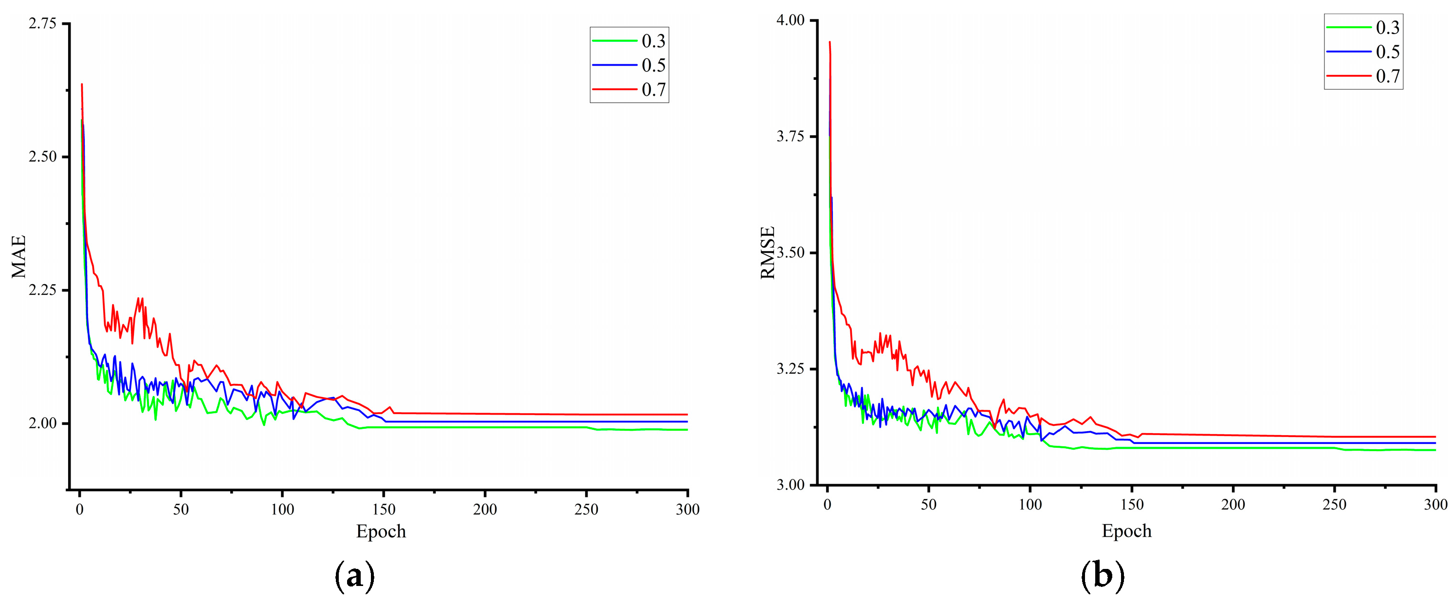
3.2.2. Model Optimization and Parameter Setting

The TG-PGAT model is optimized by incorporating elements from models such as GAT, TCN, and BiGRU. Therefore, during the TG-PGAT model experiment, it is necessary to optimize and adjust the structure parameters and training parameters. To ensure the robustness and accuracy of the model under various conditions, this paper selects or adjusts the loss function, optimizer, and random dropout. The Loss values or error comparison results for the commonly used loss functions (Mean Square Error (MSE) Loss [39], MAE Loss [40], and Huber Loss [41]), commonly used optimizers (Stochastic Gradient Descent (SGD) [42] and Admn [43]), and different random dropout parameters (0.3, 0.5, and 0.7 [44]) are shown below in Figure 10, Figure 11 and Figure 12, respectively.

The loss function is an important indicator for evaluating the training quality of machine learning models. From Figure 10, it can be seen that Huber Loss performs better in terms of final error level, robustness, and other aspects (parameter set to 1). Therefore, this paper employs Huber Loss as the loss function of the TG-PGAT traffic flow model in the port. Figure 11 shows the performance of two commonly used optimizers, SGD and Adam. It is evident that Adam converges better with increasing training iterations. In the ship traffic flow prediction model for ports, due to the complexity and nonlinearity of the data, random dropout can help the model generalize better to various traffic scenarios and conditions, thereby enhancing the accuracy and reliability of the predictions. Figure 12 shows the variations in MAE and RMSE of the model under different parameter settings. It can be seen that the overall traffic flow prediction performance is good across the three parameter values, with no significant numerical differences. The prediction effect is optimal when the parameter is set to 0.3. However, to prevent overfitting of the model and thus enhance its generalization capability, this paper chooses to set the random dropout parameter value to 0.5.

After conducting multiple experimental comparisons and optimizations, the final parameters for the TG-PGAT model training process are set as follows: the batch size of the model is 64, the maximum training times are 300, and the initial learning rate of Adam is 0.001. The main structural parameter settings of the model in the experimental process and analysis are detailed in

Table 1. Main structural parameter settings of the model.

Module	Model	Parameter	Value
Feature Decomposition	VMD	K	5
Temporal Feature Extraction	TCN	L	4
		k	5
		d	1, 2, 4, 8, 16
	BiGRU	Hidden Layer Neurons	64
Spatial Feature Extraction	GAT	Number of Layers	3
		Number of Attention Heads	4

.

3.3. Model Performance Experiment

In order to evaluate the overall prediction performance of the TG-PGAT model, the prediction effect of the model is experimentally analyzed across multi-dimensions, such as evaluation indicator errors and performance comparisons of different models.

3.3.1. Overall Prediction Effect of the Model

According to the division of the experimental dataset and the model parameter setting scheme, the training and testing set effects of the TG-PGAT model are shown in Figure 13 and Figure 14, respectively.

Figure 13 and Figure 14 reflect the overall predictive performance of the TG-PGAT model. The model fits well on both the training and testing sets, indicating its effectiveness in capturing the changing patterns of traffic flow. And the R² values of the training and testing sets are close, indicating that the model does not suffer from overfitting and has good generalization ability.

3.3.2. Comparative Analysis of Model Performance

To further demonstrate the superiority of the TG-PGAT model in predicting ship traffic flow in the port, ten classic algorithms in the field of traffic flow prediction are selected for comparative analysis across various dimensions, as shown in

Table 2. Comparison models.

Prediction Methods		Characteristics	Literature
Traditional Statistical Models	ARIMA	It has a good effect on predicting long-term traffic flow with obvious trends and seasonality but cannot handle the nonlinear characteristics of traffic flow.	[6]
	KF	It can effectively address the nonstationary characteristics of traffic flow time series and has good performance in short-term traffic flow prediction.	[1]
Classical Machine Learning Methods	SVM	It can capture the complex nonlinear relationships in traffic flow data, but the parameter settings significantly impact the prediction results.	[11]
	KNN	As a nonparametric learning method, it cannot uncover the periodic characteristics of traffic flow.	[9]
Deep Learning Models	CNN	It can capture spatial correlations by using multiple layers of convolution and nonlinear activation functions.	[15]
	TCN	It captures local temporal dependencies in time-series data through convolution operations and is sensitive to hyperparameters and data noise.	[45]
	GRU	It effectively solves the gradient vanishing or explosion problem that traditional RNNs encounter when processing long sequences, thereby being able to capture long-term dependencies in traffic flow data.	[18]
Data-Driven Spatiotemporal Fusion Models	CNN-LSTM	It can simultaneously extract the spatial and temporal features of traffic flow data, achieving a deep integration of spatiotemporal features.	[21]
	Semi-Dynamic Spatial–Temporal GNN (SDSTGNN)	It can effectively extract the spatiotemporal features of channel traffic flow by integrating GNN, LSTM, and Transformer.	[24]
	Spatial-Temporal Attention Bidirectional LSTM (STA-BiLSTM)	It can achieve spatiotemporal traffic flow prediction in inland waters by combining GAT and BiLSTM models.	[25]

.

The TG-PGAT model and ten other comparison models are analyzed using three selected evaluation indicators. At the same time, to evaluate the model’s predictive performance at various time granularities, traffic flow values are predicted for three different durations: 1 h, 2 h, and 3 h. The results of MAE, RMSE, and MAPE are shown in Figure 15.

Figure 15 shows the distribution of error indicators between TG-PGAT and ten other comparative models under different prediction durations. The prediction error indicators for all models generally increase with increasing prediction duration, suggesting that the prediction duration is a crucial factor that affects model performance. The uncertainty and complexity of long-term predictions intensify over time. The TG-PGAT model performs better than other models under different prediction durations, exhibiting relatively small errors in each indicator, particularly when contrasted with individual machine learning or deep learning models. This not only reflects the superior performance of the TG-PGAT model for traffic flow prediction in complex spatiotemporal environments in the port but also proves that the combination of temporal and spatial features is necessary for traffic flow prediction in complex navigable environments. Therefore, the results of multi-step prediction experiments validate that the TG-PGAT model can accurately capture the correlation among deep levels of spatiotemporal traffic flow features.

3.4. Ablation Experiment

Considering the periodicity and spatial correlation of ship traffic flow at various intervals in port waters, the TG-PGAT model integrates different models or methods, such as TCN, BiGRU, and GAT. To identify the importance of key factors on the prediction results and better understand the role of each module of the model, four model variants, G-PGAT (removing the local time-series feature extraction module), T-PGAT (removing the global time-domain feature extraction module), TG-GAT (removing the global spatial feature extraction module), and TG (removing the spatial feature extraction module), are designed to train using the training set. The training process is shown in Figure 16.

As can be seen from Figure 16, the loss values during the training process of both the TG-PGAT model and its variants decrease rapidly and converge promptly, but there are some differences in both the convergence speed and the convergence values. The T-PGAT model has the fastest convergence speed, followed by TG-PGAT and G-PGAT, while the TG model has the slowest convergence speed. The TG-PGPT model exhibits the lowest convergence value, followed by T-PGAT and G-PGAT. The TG model with a missing spatial feature extraction module has significantly higher errors than other models. This indicates that the addition of the graph attention mechanism can effectively capture the spatial features of ship traffic flow in the port and further reflects the importance of the in-depth extracting of spatial features for the ship traffic flow prediction in the port. It is observed that the TG-GPT model without the global spatial feature extraction module lags behind the model with the addition of this module in terms of convergence speed and value. This observation underscores the effectiveness of exploring inter-node correlation degrees through the global correlation coefficient matrix in predicting ship traffic flow in the port.

To clarify the performance of the model variants in prediction effectiveness, a comparative analysis is conducted using the quantitative values of three evaluation indicators under different durations. The results are shown in Figure 17.

As shown in Figure 17, three indicators of the model with the spatial feature extraction module are significantly lower than those of the TG variant model under different prediction durations. This reveals that spatial feature extraction is crucial for enhancing the accuracy of predicting ship traffic flow in the port. The addition of the global correlation coefficient matrix feature fusion module is also important for reducing the prediction error value, which further indicates that the module can help the model to deeply explore the hidden relationship between nodes and can better improve the spatial expression capability of the model. For the temporal feature extraction module, G-PGPT and T-PGPT perform similarly. At a predicted duration of 1 h, T-PGPT has smaller errors across all indicators than G-PGPT. However, as the prediction duration increases, the performance advantage of T-PGPT is not obvious anymore, and the errors of both models are basically similar across each indicator. This is because TCN can better capture local information in traffic flow time series, while BiGRU performs well in capturing long-term dependencies in traffic flow data. Therefore, the fusion of TCN and BiGRU temporal feature extraction modules can improve the generalization capability and adaptability of the model in traffic flow prediction.

3.5. Robustness Experiment

The above experiments mainly evaluate and compare the accuracy of the model based on evaluation indicators. For the prediction of ship traffic flow in the port, abnormal factors such as severe weather, navigation restrictions, port operation conditions, and special types of ships (such as Liquefied Natural Gas (LNG) ships) can have heterogeneous effects on the spatiotemporal features of traffic flow, resulting in significant fluctuations in traffic flow data. Therefore, validating the robustness of the prediction model is crucial to ensure its applicability in shipping practices. To this end, a set of Gaussian random noise is added to the training dataset during the model training process, with noise variances set at 0.2, 0.4, 0.6, 0.8, and 1.0. The errors in predicting durations for 1 h, 2 h, and 3 h with the added noise are then compared. The results are shown in Figure 18.

Figure 18 shows the variations in the training error indicator of the TG-PGAT model after adding Gaussian noise. Original represents the predictive effect of the model without adding noise, while 0.2, 0.4, 0.6, 0.8, and 1.0 represent the predictive effect of different noise parameter values, respectively. Overall, different noise parameter values have little influence on the model’s prediction performance. Particularly during prediction times of 1 h and 2 h, the model shows a high degree of robustness, and the evaluation indicators are almost unaffected by the fluctuation of the noise parameters. When the prediction time reaches 3 h, the cumulative effect of noise gradually manifests over time, resulting in a slight increase in the value of each evaluation indicator. While the increase is modest, the trend highlights the significance of taking noise factors into account at extended prediction time scales. This phenomenon also emphasizes the importance of incorporating the BiGRU global temporal feature extraction module into the model in this paper. Simultaneously, it also reveals the long-term impacts that unusual factors or emergencies within port waters can exert on ship traffic flow. The short-term impact may be limited, but the long-term cumulative effect may gradually evolve into significant problems, such as port congestion and ship delays, affecting the efficiency and safety of port navigation.

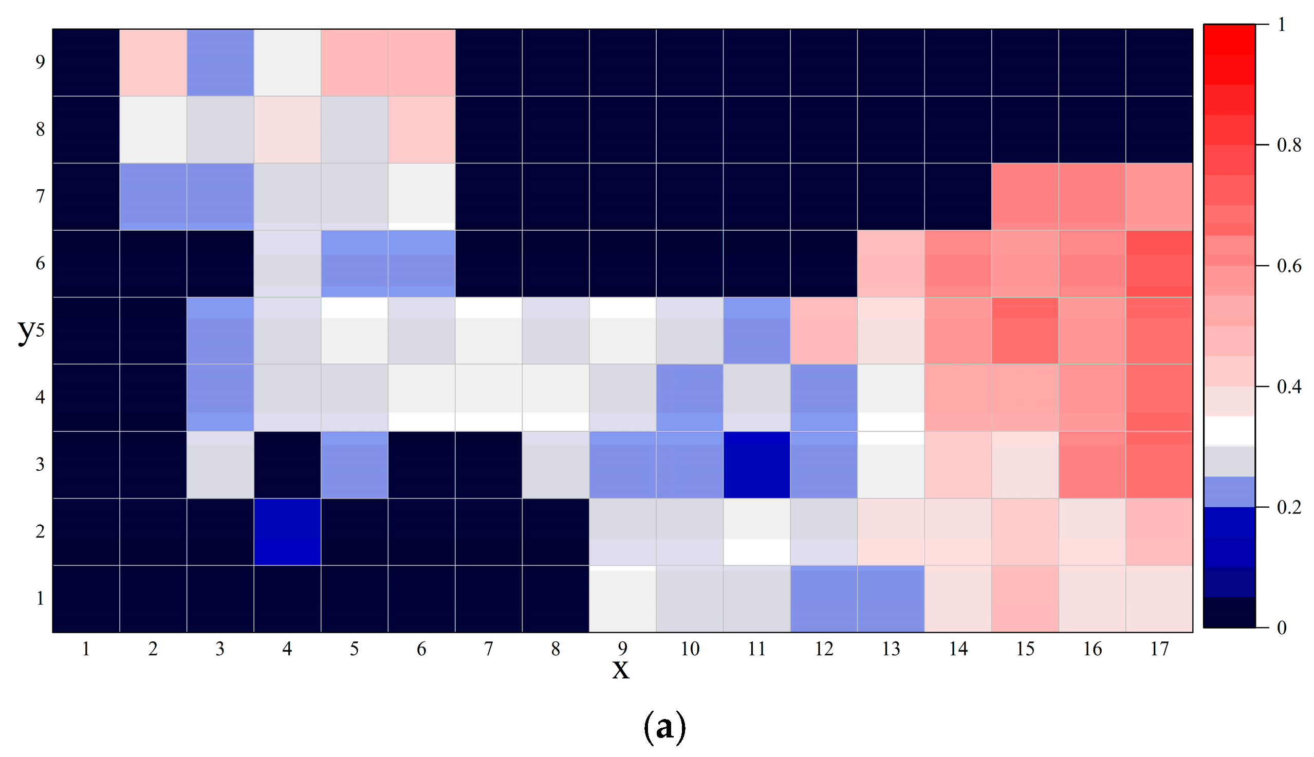
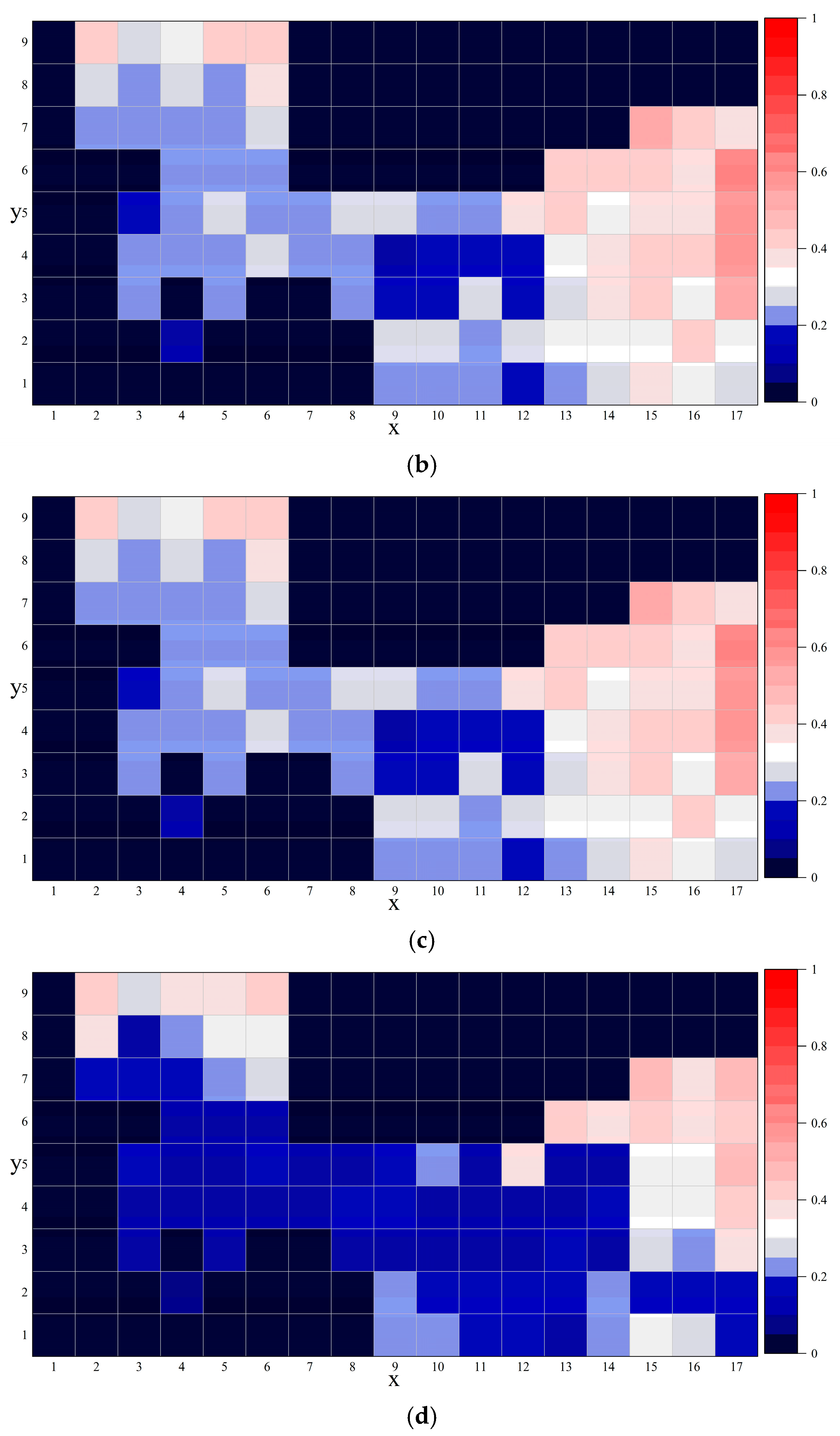
3.6. Visualization Experiment

To further validate the superiority of the TG-PGAT model in temporal and spatial traffic flow prediction and to avoid the impact of anomalies or poor performance at specific spatiotemporal nodes on the overall evaluation results of the model, several models are selected based on the characteristics of different comparative models outlined in Table 2. These models are used to visualize traffic flow variations at different time nodes within a day (taking nodes x5y5 and x10y4 in Figure 1 as examples) and the traffic flow error values at different spatial nodes in port waters, as shown in Figure 19 and Figure 20.

From Figure 19 and Figure 20, it can be observed that the ship traffic flow in the port has an obvious spatiotemporal dependence; that is, there are periodic fluctuations in traffic flow at different temporal and spatial nodes within a day. As shown in Figure 19, although the two nodes are relatively far apart and significantly differ in traffic flow, their variation trends are quite similar, both exhibiting two distinct peaks. This also demonstrates the effectiveness of incorporating the global correlation coefficient matrix into spatial feature extraction within the model. In addition, each model can fit changes in future traffic flow well. However, the prediction effect of the model integrating spatiotemporal features is obviously better than that of the single model, and the overall prediction error of node x10y4 is less than that of node x5y5.

Figure 20 compares the prediction error effects of the four models incorporating spatiotemporal features at different nodes in the port. Overall, in the key functional areas, such as port channels and anchorages, each model demonstrates a better prediction effect with error values generally below 0.3, but the error increases significantly in other peripheral areas of the port. This may be attributed to sparse data resulting from lower traffic flow in the surrounding areas. By comparison, it was found that the STA-BiLSTM and TG-PGAT models utilize the GAT-based attention mechanism to capture relevant features of spatial nodes, resulting in significantly better prediction performance in surrounding areas compared to CNN-LSTM and SDSTGNN. Additionally, the TG-PGAT model has the best predictive performance across various nodes within the port. This also proves that the model can more accurately capture the spatial dependencies of different nodes in the port after adopting the multi-head attention mechanism to establish the local features of nodes and fusing the global correlation coefficient matrices.

4. Conclusions

Accurate prediction of ship traffic flow in the port can provide forward-looking information for planning ship entry and exit routes and provide data support for more efficient and safe management of waterway resources optimization and scheduling in the port. It is an important direction for the development of maritime intelligent transportation systems. Based on the navigational characteristics of the port and the spatiotemporal features of the traffic flow, an AIS data-driven deep learning model of ship traffic flow in the port (TG-PGAT) is constructed. This model takes the GAT spatial graph model as the basis, introduces the dynamic correlation coefficient matrix, and integrates the TCN and BiGRU models. This model effectively addresses the challenges of accurately capturing long-time series data and adequately extracting dynamic spatial features in traffic flow prediction.

The TG-PGAT model innovatively constructs a module that combines GAT with the dynamic correlation coefficient matrix in the spatial feature extraction part, effectively solving the dynamic spatial features problem of ship traffic flow in the port. In the temporal feature extraction part, the combination of TCN’s efficiency in time-series processing and BiGRU’s advantage in capturing long-term dependencies enables the model to predict long-term traffic situations more accurately and efficiently. In order to demonstrate the superior performance of the TG-PGAT model, evaluation indicators are selected, and experimental analysis and comparative studies are conducted from multiple perspectives. The results show that the accuracy, robustness, and noise resistance of this model in predicting ship traffic flow in the port are significant.

The TG-PGAT model achieves traffic flow prediction based on the temporal sequence features of traffic flow and the spatial features of ports. However, the ship traffic flow in the port not only has complex and dynamic spatiotemporal dependencies but is also influenced by various external factors such as weather, channel conditions, and navigation rules. This is especially prominent in LNG-specialized ports, where the navigational rules and management requirements differ significantly. Accurately predicting traffic flow in specialized ports is, therefore, more crucial. Future research focuses on better integrating multi-source data for high-precision, long-time-step, and interpretable ship traffic flow prediction, as well as generalizing it to various types of ports.

References

1. He, W.; Zhong, C.; Sotelo, M.A.; Chu, X.; Liu, X.; Li, Z. Short-term vessel traffic flow forecasting by using an improved Kalman model. Clust. Comput. 2019, 22, 7907–7916. [Google Scholar] [CrossRef]
2. Chen, X.; Chen, H.; Yang, Y.; Wu, H.; Zhang, W.; Zhao, J.; Xiong, Y. Traffic flow prediction by an ensemble framework with data denoising and deep learning model. Phys. A 2021, 565, 125574. [Google Scholar] [CrossRef]
3. Harrou, F.; Dairi, A.; Zeroual, A.; Sun, Y. Forecasting of bicycle and pedestrian traffic using flexible and efficient hybrid deep learning approach. Appl. Sci. 2022, 12, 4482. [Google Scholar] [CrossRef]
4. Yan, Z.; Yang, H.; Guo, D.; Lin, Y. Improving airport arrival flow prediction considering heterogeneous and dynamic network dependencies. Inf. Fusion 2023, 100, 101924. [Google Scholar] [CrossRef]
5. Yan, X.; Gan, X.; Tang, J.; Zhang, D.; Wang, R. ProSTformer: Progressive space-time self-attention model for short-term traffic flow forecasting. IEEE Trans. Intell. Transp. Syst. 2024, 25, 1–15. [Google Scholar] [CrossRef]
6. Zhao, L.; Chang, D.; Zhu, Z.; Gao, Y. Port traffic volume forecast with SARIMA-BP model. Navig. China 2020, 43, 50–55. [Google Scholar]
7. Wan, J.; Li, J.; Zhang, S. Prediction model for ship traffic flow considering periodic fluctuation factors. In Proceedings of the 2018 IEEE 3rd Advanced Information Technology, Electronic and Automation Control Conference (IAEAC), Chongqing, China, 12–14 October 2018; pp. 1506–1510. [Google Scholar]
8. Zissis, D.; Xidias, E.K.; Lekkas, D. Real-time vessel behavior prediction. Evol. Syst. 2016, 7, 29–40. [Google Scholar] [CrossRef]
9. Yang, L.; Yang, Q.; Li, Y.; Feng, Y. K-nearest neighbor model based short-term traffic flow prediction method. In Proceedings of the 2019 18th International Symposium on Distributed Computing and Applications for Business Engineering and Science (DCABES), Wuhan, China, 8–10 November 2019; pp. 27–30. [Google Scholar]
10. Chen, E.Y.; Chen, R. Modeling dynamic transport network with matrix factor models: An application to international trade flow. J. Data Sci. 2023, 21, 490–507. [Google Scholar] [CrossRef]
11. Zeng, X. Ship traffic flow prediction method based on support vector machine. Ship Sci. Technol. 2023, 45, 160–163. [Google Scholar]
12. Han, X.; Liu, C.; Wang, J. Ship traffic flow prediction based on fractional order gradient descent with momentum for RBF neural network. J. Ship. Res. 2021, 65, 100–107. [Google Scholar] [CrossRef]
13. Zhao, J.; Chen, Y.; Zhou, Z.; Zhao, J.; Wang, S.; Chen, X. Extracting vessel speed based on machine learning and drone images during ship traffic flow prediction. J. Adv. Transp. 2022, 2022, 3048611. [Google Scholar] [CrossRef]
14. Chen, Y.; Huang, M.; Song, K.; Wang, T. Prediction of ship traffic flow and congestion based on extreme learning machine with whale optimization algorithm and fuzzy c-Means clustering. J. Adv. Transp. 2023, 2023, 7175863. [Google Scholar] [CrossRef]
15. Zhang, W.; Yu, Y.; Qi, Y.; Shu, F.; Wang, Y. Short-term traffic flow prediction based on spatio-temporal analysis and CNN deep learning. Transp. A Transp. Sci. 2019, 15, 1688–1711. [Google Scholar] [CrossRef]
16. Sun, Y.; Peng, X.; Ding, Z.; Zhao, J. An approach to ship behavior prediction based on AIS and RNN optimization model. Int. J. Transp. Eng. Technol. 2020, 6, 16. [Google Scholar]
17. Lee, E.; Khan, J.; Son, W.-J.; Kim, K. An efficient feature augmentation and LSTM-based method to predict maritime traffic conditions. Appl. Sci. 2023, 13, 2556. [Google Scholar] [CrossRef]
18. Xu, T.; Zhang, Q. Ship traffic flow prediction in wind farms water area based on spatiotemporal dependence. J. Mar. Sci. Eng. 2022, 10, 295. [Google Scholar] [CrossRef]
19. Li, Y.; Liang, M.; Li, H.; Yang, Z.; Du, L.; Chen, Z. Deep learning-powered vessel traffic flow prediction with spatial-temporal attributes and similarity grouping. Eng. Appl. Artif. Intell. 2023, 126, 107012. [Google Scholar] [CrossRef]
20. El Mekkaoui, S.; Benabbou, L.; Caron, S.; Berrado, A. Deep learning-based ship speed prediction for intelligent maritime traffic management. J. Mar. Sci. Eng. 2023, 11, 191. [Google Scholar] [CrossRef]
21. Ding, R.; Xie, H.; Dai, C.; Qiao, G. Research on ship traffic flow prediction based on GTO-CNN-LSTM. In Proceedings of the Seventh International Conference on Traffic Engineering and Transportation System (ICTETS 2023), Dalian, China, 22–24 September 2023; pp. 62–69. [Google Scholar]
22. Ma, Q.; Du, X.; Liu, C.; Jiang, Y.; Liu, Z.; Xiao, Z.; Zhang, M. A hybrid deep learning method for the prediction of ship time headway using automatic identification system data. Eng. Appl. Artif. Intell. 2024, 133, 108172. [Google Scholar] [CrossRef]
23. Li, Y.; Li, Z.; Mei, Q.; Wang, P.; Hu, W.; Wang, Z.; Xie, W.; Yang, Y.; Chen, Y. Research on multi-port ship traffic prediction method based on spatiotemporal graph neural networks. J. Mar. Sci. Eng. 2023, 11, 1379. [Google Scholar] [CrossRef]
24. Li, L.; Pan, M.; Liu, Z.; Sun, H.; Zhang, R. Semi-dynamic spatial–temporal graph neural network for traffic state prediction in waterways. Ocean Eng. 2024, 293, 116685. [Google Scholar] [CrossRef]
25. Man, J.; Chen, D.; Wu, B.; Wan, C.; Yan, X. An effective approach for Yangtze river vessel traffic flow forecasting: A case study of Wuhan area. Ocean Eng. 2024, 296, 116899. [Google Scholar] [CrossRef]
26. Dragomiretskiy, K.; Zosso, D. Variational mode decomposition. IEEE Trans. Signal Process. 2014, 62, 531–544. [Google Scholar] [CrossRef]
27. Okwonu, F.Z.; Asaju, B.L.; Arunaye, F.I. Breakdown analysis of pearson correlation coefficient and robust correlation methods. In Proceedings of the International Conference on Technology, Engineering and Sciences (ICTES), Penang, Malaysia, 17–18 April 2020; p. 012065. [Google Scholar]
28. Li, H.; Xing, W.; Jiao, H.; Yang, Z.; Li, Y. Deep bi-directional information-empowered ship trajectory prediction for maritime autonomous surface ships. Transp. Res. Part E Logist. Transp. Rev. 2024, 181, 103367. [Google Scholar] [CrossRef]
29. Zhang, D.; Li, X.; Wan, C.; Man, J. A novel hybrid deep-learning framework for medium-term container throughput forecasting: An application to China’s Guangzhou, Qingdao and Shanghai hub ports. Marit. Econ. Logist. 2024, 26, 44–73. [Google Scholar] [CrossRef]
30. Veličković, P.; Cucurull, G.; Casanova, A.; Romero, A.; Liò, P.; Bengio, Y. Graph attention networks. In Proceedings of the 6th International Conference on Learning Representations (ICLR 2018), Vancouver, BC, Canada, 3 May 2018; pp. 1–12. [Google Scholar]
31. Lea, C.; Vidal, R.; Reiter, A.; Hager, G.D. Temporal convolutional networks: A unified approach to action segmentation. In Proceedings of the Computer Vision–ECCV 2016 Workshops, Amsterdam, The Netherlands, 8–10 October 2016; pp. 47–54. [Google Scholar]
32. Bai, S.; Kolter, J.Z.; Koltun, V. An empirical evaluation of generic convolutional and recurrent networks for sequence modeling. arXiv 2018. [Google Scholar] [CrossRef]
33. Sun, Y.; Jiang, X.; Hu, Y.; Duan, F.; Guo, K.; Wang, B.; Gao, J.; Yin, B. Dual dynamic spatial-temporal graph convolution network for traffic prediction. IEEE Trans. Intell. Transp. Syst. 2022, 23, 23680–23693. [Google Scholar] [CrossRef]
34. Zhang, B.; Wang, S.; Deng, L.; Jia, M.; Xu, J. Ship motion attitude prediction model based on IWOA-TCN-Attention. Ocean Eng. 2023, 272, 113911. [Google Scholar] [CrossRef]
35. Luo, P.; Wang, B.; Tian, J. TTSAD: TCN-Transformer-SVDD Model for Anomaly Detection in air traffic ADS-B data. Comput. Secur. 2024, 141, 103840. [Google Scholar] [CrossRef]
36. Zhang, X.; Wen, S.; Yan, L.; Feng, J.; Xia, Y. A hybrid-convolution spatial–temporal recurrent network for traffic flow prediction. J. Comput. 2024, 67, 236–252. [Google Scholar] [CrossRef]
37. Chen, J.; Zhang, J.; Chen, H.; Zhao, Y.; Wang, H. A TDV attention-based BiGRU network for AIS-based vessel trajectory prediction. iScience 2023, 26, 106383. [Google Scholar] [CrossRef] [PubMed]
38. Li, Z.; Liu, T.; Peng, X.; Ren, J.; Liang, S. An AIS-based deep learning model for multi-task in the marine industry. Ocean Eng. 2024, 293, 116694. [Google Scholar] [CrossRef]
39. Allen, D.M. Mean square error of prediction as a criterion for selecting variables. Technometrics 1971, 13, 469–475. [Google Scholar] [CrossRef]
40. Chai, T.; Draxler, R.R. Root mean square error (RMSE) or mean absolute error (MAE)?—Arguments against avoiding RMSE in the literature. Geosci. Model Dev. 2014, 7, 1247–1250. [Google Scholar] [CrossRef]
41. Meyer, G.P. An alternative probabilistic interpretation of the huber loss. In Proceedings of the IEEE/CVF Conference on Computer Vision and Pattern Recognition (CVPR), Nashville, TN, USA, 19–25 June 2021; pp. 5261–5269. [Google Scholar]
42. Bottou, L. Large-scale machine learning with stochastic gradient descent. In Proceedings of the 19th International Conference on Computational Statistics (COMPSTAT), Paris, France, 22–27 August 2010; pp. 177–186. [Google Scholar]
43. Kingma, D.P.; Ba, J. Adam: A Method for Stochastic Optimization. arXiv 2015. [Google Scholar] [CrossRef]
44. Hinton, G.E.; Srivastava, N.; Krizhevsky, A.; Sutskever, I.; Salakhutdinov, R. Improving neural networks by preventing co-adaptation of feature detectors. arXiv 2012. [Google Scholar] [CrossRef]
45. Zhao, W.; Gao, Y.; Ji, T.; Wan, X.; Ye, F.; Bai, G. Deep temporal convolutional networks for short-term traffic flow forecasting. IEEE Access 2019, 7, 114496–114507. [Google Scholar] [CrossRef]
Figure 1. Gridded results of the study waters.
Jmse 12 01875 g001
Figure 2. Spatial influencing factors of ship traffic flow in port waters.
Jmse 12 01875 g002
Figure 3. VMD time-series decomposition of ship traffic flow in the port.
Jmse 12 01875 g003
Figure 4. Thermal map of spatial nodes related to ship traffic flow in the port.
Jmse 12 01875 g004
Figure 5. Architecture of the TG-PGAT model.
Jmse 12 01875 g005
Figure 6. The calculation of the spatial attention coefficient of ship traffic flow in the port using GAT.
Jmse 12 01875 g006
Figure 7. Fusion strategy for spatial features of ship traffic flow in the port.
Jmse 12 01875 g007
Figure 8. The architecture of the TCN model for extracting time-series features of ship traffic flow in the port (a represents the TCN neural network architecture, b represents the residual block, and c represents the dilated causal convolution).
Jmse 12 01875 g008
Figure 9. Extraction steps of temporal features of ship traffic flow in the port using BiGRU.
Jmse 12 01875 g009
Figure 10. Loss values of different loss functions.
Jmse 12 01875 g010
Figure 11. Loss values of different optimizers.
Jmse 12 01875 g011
Figure 12. Error values of different random dropout parameters. (a) MAE; (b) RMSE.
Jmse 12 01875 g012
Figure 13. Training set effect of the TG-PGAT model.
Jmse 12 01875 g013
Figure 14. Testing set effect of the TG-PGAT model.
Jmse 12 01875 g014
Figure 15. Distribution of error indicators for each model under different prediction durations. (a) prediction duration of 1 h; (b) prediction duration of 2 h; (c) prediction duration of 3 h.
Jmse 12 01875 g015
Figure 16. The training process of ablation experiment.
Jmse 12 01875 g016
Figure 17. Comparison of error indicators for prediction effects in ablation experiments. (a) MAE error; (b) RMSE error; (c) MAPE error.
Jmse 12 01875 g017aJmse 12 01875 g017b
Figure 18. Variations in evaluation indicators after adding Gaussian noise for different prediction durations.
Jmse 12 01875 g018
Figure 19. Comparison of traffic flow prediction by different models at various temporal nodes within a day. (a) node x5y5; (b) node x10y4.
Jmse 12 01875 g019
Figure 20. Distribution of traffic flow prediction error values by different models at various spatial nodes in port waters. (a) CNN-LSTM; (b) SDSTGNN; (c) STA-BiLSTM; (d) TG-PGAT.
Jmse 12 01875 g020aJmse 12 01875 g020b