Fault Tolerant Control in Underwater Vehicles

Abstract

The article discusses the problem of adaptive system synthesis to provide the detection, estimation, and elimination of the negative consequences of faults in the thrusters of underwater robots and deviations of their parameters. For this purpose, an approach consisting of three stages is proposed. At the first stage, based on a bank of diagnostic observers, deviations of the thruster parameters from their nominal values or the occurrence of errors in the readings of its sensors are detected. At the second stage, the magnitudes of the detected deviations and errors are estimated using sliding mode observers. To estimate not only single but also multiple faults, the additional sliding mode observers are used. At the third stage, a control signal is generated to retain the basic dynamic properties of the thruster based on the estimated magnitudes of deviations and errors. Thus, the main contribution of this paper is designing the systems compensating for the consequences of faults occurring in the thrusters of the UR and errors in the readings of the angular velocity sensors. This avoids reducing the accuracy of movement along specified trajectories, as well as preventing accidents that could lead to the loss of the vehicle. The operability and efficiency of the proposed systems were tested using computer simulations and experimental studies on an electro-mechanical stand.

1. Introduction

Currently, the areas of use for underwater robots (URs) and the complexity of their operations are significantly expanding [1,2,3]. The occurrence of faults that result in the deviation of the UR thrusters’ parameters from their nominal values can lead to a significant decrease in the quality of the underwater missions and operations and to various emergency situations, as well as to the loss of the expensive robots.

A general idea of ways to improve the reliability of robotic systems is suggested in [4,5,6]. One promising approach to solve this problem is the use of fault diagnosis methods for rapid fault detection and estimation followed by the generation of special control allowing the automatic preservation of the most important characteristics of the UR during its operation.

The traditional way to increase the survivability of technical systems is to increase the reliability of individual elements of these systems [7,8]. However, the use of this method applied to modern systems, operating for a long time in an aggressive marine environment, does not always give the required positive effect. In addition, the reason for failures and accidents in UR operation is often the human factor, as they are caused by personnel errors.

These errors can be identified by conducting various pre-launch tests. However, these tests provide only the most general verification of the operability of individual elements and subsystems of the UR before diving and do not identify faults that occur during the operation of the UR.

Another traditional approach to improve the reliability and survivability of responsible systems is the use of hardware redundancy when the additional elements are included in the technical systems. Such elements perform the same functions as the main elements and allow the maintenance of normal operation in case of failure. In [9], an approach to adaptive systems design that neutralizes the negative effects of faults in the thrusters of the UR is considered. It involves the shutdown of a faulty thruster with the subsequent distribution of its thrust among other additional thrusters. The disadvantage of this approach is the need to use an excessive number of thrusters in the UR. Furthermore, the addition of backup elements is limited by the maximum permissible design and operational (weight, size, energy, etc.) characteristics of the device.

An alternative approach that does not require complicating the control system is the use of diagnostic systems that allow the timely detection of emerging malfunctions in the process of the direct execution of the prescribed missions and technological operations performed by robots. Currently, the URs are equipped by control and emergency systems to assess the technical condition and identify possible malfunctions of on-board equipment. But these systems, as a rule, provide only general monitoring of the operability of the UR subsystems and when a malfunction is detected, they assume an emergency stop of the missions being performed and an ascent to the surface. In addition, these systems do not guarantee the verification of the correct functioning of individual elements of the control system, and therefore cannot detect errors in sensor readings and deviations in the parameters of robot thrusters.

To overcome these drawbacks, different fault diagnosis methods can be used which can detect the facts of the improper operation of individual elements of the UR when the faults occur. The process of fault diagnosis contains two stages: the generation of a residual and decision making. The residual is the difference between the transformed output of the actual object and the output of the diagnostic system.

There exist two main methods to generate a residual: Kalman filters [10,11,12] and asymptotically stable observers (Luenberger observers) [13,14,15]. In [16,17]. The methods of fault diagnosis in various robotic systems using extended Kalman filters are described. They are mainly focused on detecting and estimating single slowly changing faults or errors in sensor readings. In [18,19], Kalman filters are used for fault diagnosis in dynamic systems described by nonlinear differential equations. These methods use a preliminary local linearization as well as an approximate solution of the covariance equation to determine the covariance matrix of errors and the feedback matrix. For these reasons, they cannot guarantee not only the optimality, but also the stability of the filter.

In addition to Kalman filters, diagnostic observers (DOs) based on Luenberger observers [13,14,15] have been widely used in the last decades. Their main advantage is that they design the DO for systems described by nonlinear differential equations. There are methods of designing the DO for nonlinear systems; these include differential geometry [20,21,22,23] and the algebra of functions [23]. These methods make it possible to obtain an optimal solution to the diagnostic problem and minimize the dimension of the DO. However, they require rather complex analytical transformations which makes it difficult to apply them in practice.

In contrast, there exists the so-called logic-dynamic approach suggested in [24] which does not guarantee the minimum dimension of the DO but produces a simple procedure based on the methods of linear algebra.

To solve the problem of fault isolation, a bank of the DO should be used. In this situation, the determination of a malfunction is achieved through the use of a matrix of symptoms $S$ [24]. Columns of this matrix correspond to possible faults and the rows correspond to the residuals generated by the observers.

Currently, a common approach to fault estimation is the use of neural networks [25,26,27,28], including adaptive networks and networks with fuzzy logic [29,30,31]. These methods make it possible to determine the parameters of nonlinear dynamic systems in the presence of faults, as well as to compensate the detected changes. The disadvantage of these approaches is the need for preliminary complex and long-term training of neural networks, as well as the use of special test modes of their movement [32], which are not always acceptable.

Another approach for estimating the faults is the use of sliding mode observers (SMOs) [33,34,35]. These SMOs are effectively used in practice to estimate faults, as well as to design fault-tolerant systems [36,37,38]. Their disadvantage is that a number of restrictions are imposed on the mathematical model of the object of diagnosis. In particular, it is required that the so-called matching condition be fulfilled that assumes that all phase coordinates of the object must be measured by appropriate sensors, and this is not always possible in the modern UR. In addition, it is necessary that the systems under diagnosis be minimal phase.

Furthermore, SMOs in the known papers are designed on the basis of the full models of the objects under diagnosis. Therefore, SMOs have a dimension no less than the dimension of these objects, which makes it difficult to implement them in practice on on-board computers. Known approaches to determining the magnitude of errors in sensor readings using SMOs provide only an approximate solution or require observers of an increased dimension for their implementation.

The well-known least squares method [39,40,41] and algorithms based on simplified linearized models of the UR motion can be used to estimate the values of the parameters of the UR thrusters but they are effective only for linear models.

The analysis shows that the methods to design control systems for the UR can be combined into two groups. The methods of the first group ensure insensitivity to emerging faults without measuring the deviations of parameters caused by them. But the systems designed by these methods have a complex practical implementation. In addition, they are applicable and effective only for a small number of faults.

The methods of the second group are based on generating special control signals. These indicators guarantee their continued functioning and maintain the stability of the critical features of these systems even in the face of faults. These methods are often quite applicable and effective for many faults that can occur in the UR.

To compensate for the consequences of faults arising in the UR, several types of robust control systems are used. The first type includes self-adjusting systems with a reference model. The main feature of these systems is the presence of a model that has specified the dynamic properties of a faulty system. Such systems are used in both terrestrial and underwater robotics, providing high-quality control of robots using fairly simple means without identifying faulty parameters. The disadvantage of such systems is the presence of high-frequency oscillations in the self-tuning circuit that often significantly reduces the quality of compensation. In addition, during the operation of such systems, deviations in parameters from their nominal values are not evaluated, which does not allow the timely termination of the UR mission when critical faults appear. These systems do not take into account the errors that occur in the readings of the sensors.

The second type includes optimally robust adaptive systems, the advantage of which is their sufficiently high robustness to uncertain parameters of the control objects. But to design such systems, linearized models should be used, which limits their application in the spatial movement of objects.

The third type of fault-tolerant control systems includes systems with a variable structure [37,38]. The disadvantage of these systems is that, in order to ensure the operability of systems with a variable structure over the entire range of changes in the parameters, they are designed taking into account the “worst case” when their parameters reduce the system performance. As a result, even in the absence of faults, additional control signals are generated, increasing the amplitude of the control signals and energy consumption and reducing the battery life of the device.

To stabilize the dynamic properties of thrusters when their parameters change, the well-known method of the synthesis of adaptive control systems can be used [24]. However, the current control systems that employ this approach do not account for potential malfunctions in the thrusters or inaccuracies in the readings of the angular velocity sensors.

As a result, the analysis shows that due to the high complexity of the implementation of the obtained control laws or low speed, most of the considered methods cannot be used to design the systems compensating for the consequences of faults occurring in the thrusters and sensors.

The main contribution of this paper is designing the systems compensating for the consequences of faults occurring in the thrusters of the UR and errors in the readings of the angular velocity sensors. The components of such systems are diagnostic and sliding mode observers for detecting, isolating, and estimating the faults and errors followed by compensating for the consequences of their appearance. These observers are of minimal dimension, which allows them to be used in on-boat computers.

The article will be organized as follows. In Section 2.1, a mathematical model of the propulsion system is described, taking into account possible faults. Section 2.2 provides a method for creating a DO bank to isolate faults. Section 2.3 describes a method for constructing SMOs to identify the values of previously isolated faults. In Section 2.4, the construction of additional observers is described, which makes it possible to simultaneously identify the values of two faults that have occurred. In Section 2.5, a synthesis of the compensation system for previously isolated and identified faults is presented, as well as the verification of its operation using computer modeling. In Section 3, the results of an experimental study of the developed systems on a special electromechanical stand is presented. Section 4 concludes the paper.

2. Methods

2.1. Mathematical Model of the UR Thruster and Its Faults

The operation of the URs shows that the occurrence of faults in their thrusters as well as errors in the angular velocity sensors, can lead to a significant decrease in UR movement accuracy along spatial trajectories or emergency situations (in exceptional cases, to a loss of the expensive robots). To develop a method of fault diagnosis, it is firstly necessary to create adequate mathematical models of thrusters, taking into account all frequently occurring faults.

UR thrusters usually use DC electric motors or motors with permanent magnets which are equipped with angular velocity sensors for their output shafts and armature circuit current sensors [24]. A full mathematical model of the underwater vehicle’s dynamics is described in [42]. It is known [24] that each individual thruster with possible faults can be described by a system of differential equations of the form

$${\dot{x}}_1\left(t\right)=-{\displaystyle \frac{k_v}{J_{\mathrm{m}}}}{x}_1\left(t\right)+{\displaystyle \frac{k_m}{J_m}}{x}_2\left(t\right)-{\displaystyle \frac{M_e\left(x_1\left(t\right), t\right)+{\widehat{M}}_e\left(t\right)}{J_m}},$$

(1)

$${\dot{x}}_2\left(t\right)=-{\displaystyle \frac{k_{\mathsf{\omega }}}{L_m}}{x}_1\left(t\right)-{\displaystyle \frac{R_m+{\widehat{R}}_m(t)}{L_m}}{x}_2\left(t\right)+{\displaystyle \frac{k_u}{L_m}}u\left(t\right),$$

with the measurements

$$y_1\left(t\right)=x_1\left(t\right)+\widehat{\omega }\left(t\right),\hspace{1em}{y}_2(t)=x_2(t),$$

where $x_1=\omega (t)$ is the angular velocity for their output shafts and $x_2=I_m(t)$ is the armature circuit current; $u\left(t\right)$ is the input voltage; $L_m$ and $R_m$ are the inductance and electrical resistance the of the armature circuit, respectively; $k_{\mathsf{\omega }}$ is back-emf coefficient; $k_u$ is the power amplifier gain; $k_m$ is the torque coefficient; $k_v$ is the coefficient of viscous friction; $M_e(x_1(t),t)$ is the moment on the propeller shaft from the interaction of the propeller with a viscous environment; and $p_{\tau }, q_{\tau }$, and ${\upsilon }_p$ are auxiliary variables.

$$M_e\left(x_1\left(t\right), t\right)=F_m\left(s_{\tau }+H_H{C}_r{x}_1\left(t\right)\right)\left|x_1\left(t\right)\right|-C_m{\displaystyle \frac{S_d\rho \left|\upsilon \left(t\right)\right|\upsilon \left(t\right)}{2\left(1+C_{\omega }{x}_1^2\left(t\right)\right)}},$$

$$s_{\tau }=p_{\tau }-sign\left(x_1\left(t\right)\right)\sqrt{{p_{\tau }}^2-q_{\tau }}, p_{\tau }=H_H{x}_1\left(t\right)-{\displaystyle \frac{{\upsilon }_p}{2}}+{\displaystyle \frac{F_{\tau }{x}_1\left(t\right)}{4\rho S_d}},$$

(2)

$$q_{\tau }=H_{\mathrm{H}}{x}_1\left(t\right)\left(H_H{x}_1\left(t\right)-{\upsilon }_p\right), H_H=H_G+{\delta }_{H}sign(x_1\left(t\right)),$$

$${\upsilon }_p=\left\{\begin{array}{c}\upsilon \left(t\right),\hspace{0.33em}\mathrm{i}\mathrm{f} sign\left(x_1\left(t\right)\right)=sign\left(\upsilon \left(t\right)\right),\\ 0, \mathrm{i}\mathrm{f} sign\left(x_1\left(t\right)\right)\ne sign\left(\upsilon \left(t\right)\right),\end{array}\right.$$

$\upsilon (t)$ is the speed of the movement of the surrounding fluid along the propeller axis relative to the UR; $H_H$ and $H_G$ are hydrodynamic and geometric pitches of the propeller; ${\delta }_H$ is the hydrodynamic correction for propeller pitch; $F_m$ is the generalized torque coefficient; $C_f$ and $C_m$ are coefficients of lift and propeller torque at $\omega (t)=0$; $C_{\omega }$ is the coefficient characterizing the decrease in lift and propeller torque at $\omega (t)\ne 0$; $C_r$ is the propeller profile loss coefficient; $\rho$ is a density of the surrounding liquid; $S_d$ is the area of the propeller disk; $J_m$ is the moment of the inertia of the rotating parts of the thruster taking into account the added moment of the inertia of the liquid; and $s_{\tau }$ is the absolute slip of the propeller.

The following typical faults can occur in the thruster:

(1)

Errors in readings of angular velocity sensors resulting in the errors $\widehat{\omega }(t)$;

(2)

A deviation ${\widehat{R}}_m(t)$ of the active resistance of the motor armature circuit from its nominal value due to the excessive heating of the motor or a short circuit of the winding turns;

(3)

The unknown external moment ${\widehat{M}}_e(t)$ on the output shafts of the propellers.

The block diagram of the thruster described by the system of Equations (1) and (2) is shown in Figure 1.

To develop the method to design DOs, rewrite (1) in the matrix form as follows:

$$\dot{x}\left(t\right)=Ax\left(t\right)+Bu\left(t\right)+\varphi \left(x\left(t\right),t\right)+Dd\left(t\right),$$

(3)

$$y(t)=\mathrm{C}x(t)+D_s\widehat{\omega }(t)$$

where $A\in R^{2\times 2}$ is the matrix of dynamic properties of the thruster; $x(t)\in R^{2\times 1}$ is the state vector; $B\in R^{2\times 1}$ is the matrix-column of gain coefficients; $y(t)\in R^{2\times 1}$ are state variables measured by sensors; $D\in R^{2\times 2}$ is the faults matrix indicating the location of faults; $d(t)\in R^{2\times 1}$ is a vector characterizing faults (in the absence of faults, all elements of the vector $d(t)$ are equal to zero, and when they appear, a specific element becomes non-zero); $C\in R^{2\times 2}$ is the output matrix; $\varphi (x\left(t\right),t)\in R^2$ is the vector function that takes into account the nonlinearities of the electric drive; and $D_s\in R^{2\times 1}$ is the vector of faults in sensors of the thruster, indicating the sensor in which the fault occurred.

Recorded in (3), the matrices and vectors have the following form:

$$\begin{array}{c}A=\left[\begin{array}{cc}-{\displaystyle \frac{k_v}{J_m}}& {\displaystyle \frac{k_m}{J_m}}\\ -{\displaystyle \frac{k_{\mathsf{\omega }}}{L_m}}& -{\displaystyle \frac{R_m}{L_m}}\end{array}\right], B=\left[\begin{array}{c}0\\ {\displaystyle \frac{k_u}{L_m}}\end{array}\right], C=\left[\begin{array}{cc}1& 0\\ 0& 1\end{array}\right], D=\left[\begin{array}{cc}1& 0\\ 0& 1\end{array}\right],\\ D_s=\left[\begin{array}{c}1\\ 0\end{array}\right],\end{array}$$

$$\varphi (x\left(t\right),t)=\left[\begin{array}{c}-{\displaystyle \frac{M_e\left(x_1\left(t\right), t\right)}{J_m}}\\ 0\end{array}\right], x(t)=\left[\begin{array}{c}\omega (t)\\ I_m(t)\end{array}\right], y(t)=\left[\begin{array}{c}{y}_1(t)\\ y_2(t)\end{array}\right]=\left[\begin{array}{c}\omega \left(t\right)+\widehat{\omega }(t)\\ I_m(t)\end{array}\right]$$

$$d\left(t\right)=\left[\begin{array}{c}{d}_1(t)\\ d_2(t)\end{array}\right]$$

where $d_1\left(t\right)=-{\displaystyle \frac{{\widehat{M}}_e\left(t\right)}{J_m}}, d_2(t)=-{\displaystyle \frac{{\widehat{R}}_m}{L_m}}{I}_m(t)$.

The model (3) will be used to synthesize a bank of DOs and to solve the problem of fault diagnosis. Each observer of the bank must be synthesized in such a way that the generated residuals are sensitive to the occurrence of various combinations of non-zero functions $d_1(t){, d}_2(t)$, and $\widehat{\omega }(t)$.

2.2. Bank of DO Design for Fault Isolation in Thrusters

To isolate faults in thrusters described by nonlinear differential Equation (3), the bank of DOs should be used. To design DOs in such a bank, we will use the logical-dynamic approach [24], which allows the study of nonlinear systems only by linear methods. In contrast to the typical logical-dynamic approach that provides the sensitivity of the DO to strictly specified faults only, a new algorithm is developed which enables the design of observers sensitive to various sets of faults.

The logical-dynamic approach consists of the following three stages:

(1)

The transformation of the original nonlinear dynamic model (3) into a linear one by discarding the nonlinear term $\varphi (x\left(t\right), t)$;

(2)

Solving (using a special algorithm) the problem of designing a bank of linear DOs, which should ensure the rapid detection of the appearance in (3) of the specific non-zero functions $d_1(t)$, $d_2(t)$, and $\widehat{\omega }(t)$;

(3)

The calculation of the additional nonlinear components by algebraic methods and their addition to the linear DO designed at the second stage.

After discarding the component $\varphi (x\left(t\right),t)$, the system (3) takes the form

$$\dot{x}\left(t\right)=Ax\left(t\right)+Bu\left(t\right)+Dd\left(t\right),$$

(4)

$$y(t)=\mathrm{C}x(t)+D_s\widehat{\omega }(t).$$

At the second stage, the linear DO are designed. Every DO is described as follows:

$${\dot{x}}_{*}\left(t\right)=A_{*}{x}_{*}\left(t\right)+B_{*}u\left(t\right)+J_{*}y\left(t\right)+K_{*}{e}_y\left(t\right),$$

(5)

$$y_{*}(t)=C_{*}{x}_{*}(t),$$

where $x_{*}(t)\in R^{k\times 1}$ is the state vector; $y_{*}(t)\in R^1$ is the output signal; $A_{*}\in R^{k\times k}$, $B_{*}(t)\in R^{k\times 1}$, $C_{*}\in R^{1\times k}$, and $J_{*}\in R^{k\times 2}$ are matrices to be determined; $K_{*}\in R^{k\times 1}$ is the matrix of the observer’s feedback coefficients; $e_y\left(t\right) \in R^1$ is the residual generated by the DO; and $k\le 2$ is the dimension of the DO.

The residual $e_y\left(t\right)$ should be sensitive to one or more non-zero functions $d_1(t)$, $d_2(t)$, and $\widehat{\omega }\left(t\right)$. If all of these functions are equal to zero, $e_y\left(t\right)=0$, otherwise $e_y\left(t\right)\ne 0$. The residual is determined as follows:

$$e_y\left(t\right)=R_{*}y(t)-y_{*}(t)$$

(6)

with the matrix $R_{*}\in R^{1\times 2}$ to be determined.

Introduce the matrix ${\mathsf{\Phi }}_{*}$ satisfying the condition

$${\mathsf{\Phi }}_{*}x\left(t\right)=x_{*}\left(t\right)$$

(7)

when $d_1\left(t\right)=0$, $d_2\left(t\right)=0$, and $\widehat{\omega }\left(t\right)=0$. It is known that the matrices describing the system and the DO satisfy the conditions

$${\mathsf{\Phi }}_{*}A=A_{*}{\mathsf{\Phi }}_{*}+J_{*}\mathrm{C}, B_{*}={\mathsf{\Phi }}_{*}B,$$

(8)

$$R_{*}C=C_{*}{\mathsf{\Phi }}_{*}.$$

According to the proposed method, each specific DO should be constructed in such a way that the appropriate residual $e_y\left(t\right)$ is sensitive to the appearance of non-zero functions $d_1(t)$, $d_2(t)$, and $\widehat{\omega }\left(t\right)$. That is, the obtained relations must be supplemented with the conditions of the sensitivity and insensitivity of the DO to these functions. To do this, rewrite expression (6) taking into account (3), (5), (7), and (8):

$$e_y\left(t\right)=R_{*}{D}_s\widehat{\omega }\left(t\right)+C_{*}({\mathsf{\Phi }}_{*}x(t)-x_{*}(t)).$$

(9)

Differentiating (9) with respect to time and taking into account (3), (5), and (8), one obtains

$${\dot{e}}_y\left(t\right)=R_{*}{D}_s\dot{\widehat{\omega }}\left(t\right)+{\mathrm{C}}_{*}(A_{*}e(t)+{\mathsf{\Phi }}_{*}Dd(t)-$$

(10)

$$-J_{*}{D}_s\widehat{\omega }\left(t\right)-K_{*}{e}_y\left(t\right)),$$

where

$$e\left(t\right)={\mathsf{\Phi }}_{*}x\left(t\right)-x_{*}\left(t\right)\in R^{k\times 1}.$$

(11)

From (10) and (11), one obtains the conditions of the sensitivity and insensitivity of the residual as follows:

• The residual $e_y(t)$ is sensitive to $d_{i_{*}}(t)$ if

$${\mathsf{\Phi }}_{*}{D}_{i_{*}}\ne 0;$$

(12)

• It is insensitive to $d_{i_{*}}(t)$ if

$${\mathsf{\Phi }}_{*}{D}_{i_{*}}=0;$$

(13)

• It is sensitive to $\widehat{\omega }\left(t\right)$ if

$$R_{*}{D}_s\ne 0 \mathrm{or} J_{*}{D}_s\ne 0;$$

(14)

• It is insensitive to $\widehat{\omega }\left(t\right)$ if

$$R_{*}{D}_s=0 \mathrm{and} J_{*}{D}_s=0.$$

(15)

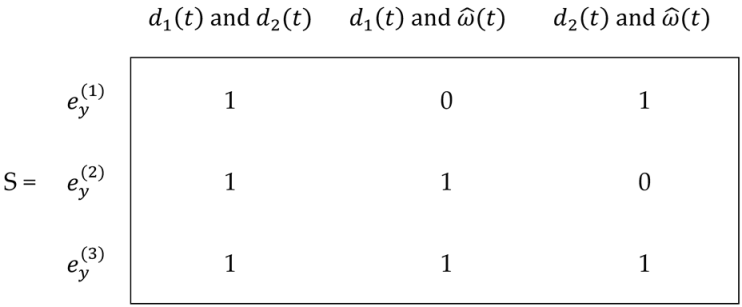
The decision on the appearance of a specific fault is made on the basis of the matrix of syndromes $S$. If the $i$-th DO is sensitive to the $j$-th fault, then $S_{i,j}=1$, otherwise $S_{i,j}=0$. If columns of the matrix $S$ are different, the faults can be isolated.

It is known [24] that the linear DO (5) design is performed easily if these observers are specified in the canonical form when

$$A_{*}=\left[\begin{array}{ccccc}0& 1& 0& \cdots & 0\\ 0& 0& 1& \cdots & 0\\ ⋮& ⋮& ⋮& \ddots & ⋮\\ 0& 0& 0& \cdots & 0\end{array}\right]{, C}_{*}=\left[\begin{array}{ccccc}1& 0& 0& \cdots & 0\end{array}\right]$$

(16)

In this case, Equation (8) can be represented as a set of $k$ equations as follows:

$${\mathsf{\Phi }}_{\ast 1}A\left(t\right)={\mathsf{\Phi }}_{\ast 2}+J_{\ast 1}\mathrm{C}$$

$${\mathsf{\Phi }}_{\ast i}A={\mathsf{\Phi }}_{\ast i+1}+J_{\ast i}\mathrm{C}, i=\overline{2,\dots ,k-1}$$

(17)

$${\mathsf{\Phi }}_{\ast k}A=J_{\ast k}\mathrm{C}$$

where ${\mathsf{\Phi }}_{\ast i}$ and $J_{\ast i}$ are the $i$th rows of the matrices ${\mathsf{\Phi }}_{*}$ and $J_{*}$, respectively. It is known that these equations can be transformed into the single one as follows:

$$R_{*}C{A}^k=J_{\ast 1}C{A}^{k-1}+J_{\ast 2}C{A}^{k-2}+\cdots +J_{\ast k}C$$

(18)

To determine the elements of the vector $K_{*}$, the Equation (10) can be written taking into account (8) under $d_1\left(t\right)=0$, $d_2\left(t\right)=0$, and $\widehat{\omega }\left(t\right)=0$ as follows:

$$\dot{e}\left(t\right)=(A_{*}-K_{*}{\mathrm{C}}_{*})e\left(t\right).$$

(19)

It follows from (19) that to obtain a stabile linear DO, the matrix $A_{*}-K_{*}{\mathrm{C}}_{*}$ must have eigenvalues with negative real parts. Let $k_{\ast 1}, k_{\ast 2}, \dots , k_{\ast k}$ be the components of the feedback matrix $K_{*}$, then

$$A_{*}-K_{*}{\mathrm{C}}_{*}=\left[\begin{array}{ccccc}-k_{\ast 1}& 1& 0& \dots & 0\\ -k_{\ast 2}& 0& 1& \dots & 0\\ ⋮& ⋮& ⋮& \dots & ⋮\\ -k_{\ast k}& 0& 0& \dots & 0\end{array}\right].$$

The coefficients $k_{\ast 1}, k_{\ast 2}, \dots , k_{\ast k}$ related to the prescribed eigenvalues ${\lambda }_1,{ \lambda }_2, \dots , {\lambda }_k$ are given by

$$k_{\ast 1}={-(\lambda }_1+{\lambda }_2+\cdots +{\lambda }_k),$$

$$k_{\ast 2}={\lambda }_1{\lambda }_2+{\lambda }_1{\lambda }_3+\cdots +{\lambda }_{k-1}{\lambda }_k,$$

(20)

$$\dots$$

$$k_{\ast k}=(-1{)}^k{\lambda }_1{\lambda }_2\dots {\lambda }_k$$

To solve Equation (18), the following new algorithm is proposed (Algorithm 1).

Algorithm 1: New algorithm To solve Equation (18)
1:	$\mathrm{Take} k=1$.
2:	If (18) has a solution, find the matrices $J_{*}$ and $R_{*}$. Otherwise, go to step 3. If the number of equations in (18) is smaller than the number of variables of the matrices $J_{*}$ and $R_{*}$, then some of these elements can be taken as free variables, and the rest of the elements express through them; go to step 4.
3:	Take $k=k+1$ and go to step 2.
4:	Find the rows of the matrix ${\mathsf{\Phi }}_{*}$ according to the following relations obtained from (8) and (16): $$\begin{array}{c}{\mathsf{\Phi }}_{\ast 1}=R_{*}C,\\ {\mathsf{\Phi }}_{\ast 2}={\mathsf{\Phi }}_{\ast 1}A-J_{\ast 1}\mathrm{C}=R_{*}\mathrm{C}A-J_{\ast 1}\mathrm{C},\\ {\mathsf{\Phi }}_{\ast 3}=R_{*}\mathrm{C}{A}^2-J_{\ast 1}\mathrm{C}A-J_{\ast 2}\mathrm{C},\\ \dots \\ {\mathsf{\Phi }}_{\ast k}=R_{*}\mathrm{C}{A}^{k-1}-J_{\ast 1}\mathrm{C}{A}^{k-2}\dots -J_{\ast k-1}\mathrm{C}.\end{array}$$
	The elements of ${\mathsf{\Phi }}_{*}$ may depend on previously accepted free variables.
5:	Check the obtained matrices ${\mathsf{\Phi }}_{*}$, $J_{*}$, and $R_{*}$ for sensitivity or insensitivity to various combinations of non-zero functions $d_1(t)$, $d_2(t)$, and $\widehat{\omega }\left(t\right)$ using criteria (12)–(15). The values of all free variables should be selected in such a way that the vector $R_{*}$ is non-zero. If it is not possible to fulfill these criteria, return to step 3.
6:	Calculate the matrix $B_{*}$ using (8).

As a result, the linear DO (5) sensitive to the combinations of non-zero functions $d_1(t)$, $d_2(t)$, and $\widehat{\omega }\left(t\right)$ has been constructed.

At the third stage of the proposed approach, the nonlinear component ${\varphi }_{*}(x_{*}\left(t\right), y\left(t\right), t)$ is added to the designed linear DO which is calculated using expression [24]

$${\varphi }_{*}\left(x_{*}\left(t\right), y\left(t\right), t\right)={\mathsf{\Phi }}_{*}\varphi (x\left(t\right), t)$$

(21)

The final description of each DO has the following form:

$${\dot{x}}_{*}\left(t\right)=A_{*}{x}_{*}\left(t\right)+B_{*}u\left(t\right)+J_{*}y\left(t\right)+{\varphi }_{*}(x_{*}\left(t\right),y\left(t\right),t)+K_{*}{e}_y\left(t\right),$$

(22)

$$y_{*}(t)=C_{*}{x}_{*}(t).$$

If ${\varphi }_{*}(x_{*}\left(t\right), y\left(t\right), t)$ = 0, the elements of the feedback matrix $K_{*}$ are calculated using (20). Otherwise, the matrix $K_{*}$ can be found based on [43].

Based on the algorithm, one can construct a bank of DOs which are sensitive only to a certain set of functions $d_1\left(t\right),d_2\left(t\right)$, and $\widehat{\omega }\left(t\right)$. The implementation of the above procedure to design a bank for isolating faults in thrusters provides the following results.

DO-1 of the first order is sensitive to the non-zero functions $d_2(t)$ and $\widehat{\omega }\left(t\right)$, but insensitive to $d_1(t)$ as follows:

$${\dot{x}}_{*}^{\left(1\right)}\left(t\right)=-{\displaystyle \frac{k_{\mathsf{\omega }}}{L_m}}{y}_1\left(t\right)-{\displaystyle \frac{R_m}{L_m}}{y}_2\left(t\right)+{\displaystyle \frac{k_u}{L_m}}u\left(t\right)+e_y^{\left(1\right)}\left(t\right),$$

(23)

$$y_{*}^{\left(1\right)}\left(t\right)=x_{*}^{\left(1\right)}\left(t\right),\hspace{1em} e_y^{(1)}(t)=y_2(t)-y_{*}^{(1)}(t).$$

DO-2 of the first order is sensitive to $d_1(t)$ and $\widehat{\omega }\left(t\right)$, but is insensitive to $d_2(t)$ as follows:

$${\dot{x}}_{*}^{\left(2\right)}\left(t\right)=-{\displaystyle \frac{k_v}{J_m}}{y}_1\left(t\right)+{\displaystyle \frac{k_m}{J_m}}{y}_2\left(t\right)-{\displaystyle \frac{M_e\left(t\right)}{J_m}}+e_y^{\left(2\right)}\left(t\right),$$

(24)

$$y_{*}^{\left(2\right)}\left(t\right)=x_{*}^{\left(2\right)}\left(t\right), \hspace{1em}{e}_y^{(2)}(t)=y_1(t)-y_{*}^{(2)}(t).$$

DO-3 of the second order is sensitive to $d_1(t)$ and $d_2(t)$, but is insensitive to $\widehat{\omega }\left(t\right)$ as follows:

$${\dot{x}}_{\ast 1}^{\left(3\right)}\left(t\right)=x_{\ast 2}^{\left(3\right)}\left(t\right)+\left(-{\displaystyle \frac{k_v}{J_m}}-{\displaystyle \frac{R_m}{L_m}}\right)y_2\left(t\right)+{\displaystyle \frac{k_u}{L_m}}u\left(t\right)+2e_y^{(3)}\left(t\right),$$

$${\dot{x}}_{\ast 2}^{\left(3\right)}\left(t\right)=\left(-{\displaystyle \frac{k_m{k}_{\mathsf{\omega }}}{J_m{L}_m}}-{\displaystyle \frac{k_v{R}_m}{J_m{L}_m}}\right)y_2\left(t\right)+{\displaystyle \frac{k_v{k}_u}{J_m{L}_m}}u\left(t\right)+{\displaystyle \frac{M_e\left(x_{*}\left(t\right),t\right)k_{\mathsf{\omega }}}{J_m{L}_m}}+e_y^{(3)}\left(t\right),$$

(25)

$$y_{*}^{\left(3\right)}\left(t\right)=x_{\ast 1}^{\left(3\right)}\left(t\right),\hspace{1em}{e}_y^{\left(3\right)}\left(t\right)=y_2\left(t\right)-y_{*}^{\left(3\right)}\left(t\right).$$

It can be shown that the matrix ${\mathsf{\Phi }}_{*}$ for DO-3 is given by

$${\mathsf{\Phi }}_{*}^{(3)}=\left[\begin{array}{cc}0& 1\\ -{\displaystyle \frac{k_{\mathsf{\omega }}}{L_m}}& {\displaystyle \frac{k_v}{J_m}}\end{array}\right]$$

(26)

The bank of DOs (23)–(25) makes it possible to determine the fact of the appearance of non-zero functions ${\widehat{M}}_e(t)$, ${\widehat{R}}_m(t)$ (or the functions $d_1(t)$ and $d_2(t)$ dependent on them), and $\widehat{\omega }\left(t\right)$ caused by the occurrence of the corresponding faults in the thrusters of the UR. For this bank, the matrix of syndromes S is given by

$$S=\left(\begin{array}{ccc}0& 1& 1\\ 1& 0& 1\\ 1& 1& 0\end{array}\right).$$

(27)

DOs (24)–(25) allow the timely detection and isolation of single faults appearing in the UR thrusters. However, they do not identify the magnitude of faults, which is necessary for further compensation of the negative consequences of their occurrence.

2.3. Bank of SMO Design for Fault Estimation

To solve the problem of fault estimation, SMOs are traditionally used. The theory for such observer design is described in many works [44]. SMOs in these papers, as a rule, are designed on the basis of full models of the object under diagnosis which makes their practical implementation difficult when using standard onboard computers of underwater robots.

Using the DOs obtained in the previous section, it is possible to modify them in order to design the SMOs. In particular, one can see from (23) and (24) that the synthesized DO-1 and DO-2 are described by simple first-order differential equations, and the generated residuals are sensitive to different functions $d_1(t)$, $d_2(t)$, or $\widehat{\omega }\left(t\right)$.

Since the functions $d_1(t)$ and $d_2(t)$ correspond to ${\widehat{M}}_e(t)$ and ${\widehat{R}}_m$ by the relations $d_1\left(t\right)=-{\displaystyle \frac{{\widehat{M}}_e\left(t\right)}{J_{\mathrm{m}}}}, d_2(t)=-{\displaystyle \frac{{\widehat{R}}_m}{L_m}}{I}_m(t)$, it is possible to obtain the values for the external torque ${\widehat{M}}_e(t)$ and the deviation of the active resistance ${\widehat{R}}_m$ from its nominal value.

To design the SMO, supplement (5) with the nonlinear term and fault:

$${\dot{x}}_{*}(t)=A_{*}{x}_{*}(t)+B_{*}u(t)+J_{*}y(t)+{\varphi }_{*}(x_{*}\left(t\right),y\left(t\right),t)+D_{*}d(t),$$

(28)

$$y_{*}(t)=C_{*}{x}_{*}(t),\hspace{1em}{D}_{*}={\mathsf{\Phi }}_{*}D.$$

Unlike DO (23), the SMO contains the discontinuous function $z(t)$:

$${\dot{\widehat{x}}}_{*}\left(t\right)=A_{*}{\widehat{x}}_{*}(t)+B_{*}u\left(t\right)+J_{*}y\left(t\right)+{\varphi }_{*}\left(x_{*}\left(t\right),y\left(t\right),t\right)-Lz\left(t\right)-K_{*}{e}_y\left(t\right),$$

(29)

$${\widehat{y}}_{*}\left(t\right)=C_{*}{\widehat{x}}_{*}\left(t\right),{{\hspace{1em}e}_y\left(t\right)=\widehat{y}}_{*}\left(t\right)-R_{*}y(t),$$

where $z\left(t\right)=g sign\left(e_y\left(t\right)\right)$ is a discontinuous function, and $L$ and $g>0$ are constant coefficients.

Using (28) and (29) for $k=1$, $A_{*}=0$, and $C_{*}=1$, one obtains

$$\dot{e}\left(t\right)={\dot{\widehat{x}}}_{*}\left(t\right)-{\dot{x}}_{*}\left(t\right)$$

(30)

$$=-K_{*}e\left(t\right)+{\Delta \varphi }_{*}\left(x_{*}\left(t\right),y\left(t\right),t\right)-Lz\left(t\right)-D_{*}d\left(t\right),$$

where $\Delta {\varphi }_{*}\left(x_{*}\left(t\right),y\left(t\right),t\right)={\varphi }_{*}\left({\widehat{x}}_{*}\left(t\right),y\left(t\right),t\right)-{\varphi }_{*}\left(x_{*}\left(t\right),y\left(t\right),t\right)$. Since the maximum value of the torque on the propeller shaft from the interaction of the screw with a viscous medium is bounded ($\left|M_e\left(t\right)\right|\le M_{max}$), then the functions ${\varphi }_{*}\left({\widehat{x}}_{*}\left(t\right),y\left(t\right),t\right)$ and ${\varphi }_{*}\left(x_{*}\left(t\right),y\left(t\right),t\right)$ are also bounded and the function $\Delta {\phi }_{*}$ is bounded as well: $\Delta {\varphi }_{*}\left(x_{*}\left(t\right),y\left(t\right),t\right)\le \Delta {\varphi }_{\ast max}$. The elements of the vector $d(t)$ associated with the values ${\widehat{M}}_e(t)$ and ${\widehat{R}}_m$ are assumed to be also bounded: $\left|d\left(t\right)\right|\le d_{max}$.

Introduce into consideration the Lyapunov function $V=0.5e^2(t)$. As is known, the equilibrium position $e\left(t\right)=0$ will be stable if the condition $\dot{V}<0$ is met. Differentiating the function $V$ with respect to time and taking into account (30), one obtains

$$\begin{gathered} \dot{V}=e\left(t\right)\dot{e}\left(t\right) \\ =e\left(t\right)\left(-K_{*}e\left(t\right)+\Delta {\varphi }_{*}\left({\widehat{x}}_{*}\left(t\right),y\left(t\right),t\right)-Lz\left(t\right)-D_{*}d\left(t\right)\right) \\ \le -K_{*}{e}^2\left(t\right)+e\left(t\right)(\Delta {\varphi }_{\ast max}-Lg sign\left(e\left(t\right)\right)+|\left|D_{*}\right|{|d}_{max}) \end{gathered}$$

Obviously, when the inequalities for $K_{*}$, $L$, and $g$ are satisfied

$$K_{*}>0,$$

(31)

$$Lg>\Delta {\varphi }_{\ast max}+\left|\left|D_{*}\right|\right|d_{max},$$

the inequality $\dot{V}<0$ will always be satisfied. Really, if $e(t)>0$, then $\dot{V}<0$ due to (31); if $e(t)<0$, then $\Delta {\phi }_{\ast max}+Lg+\left|\left|D_{*}\right|\right|d_{max}>0$ and $\dot{V}<0$ as well.

If conditions (31) are met, the relations $e\left(t\right)\to 0$ and $\dot{e}\left(t\right)\to 0$ will be fulfilled for the first-order SMOs in a finite amount of time. Thus, the expression ${\widehat{x}}_{*}\left(t\right)=x_{*}\left(t\right)$ is valid, and therefore ${\Delta \varphi }_{*}\left(x_{*}\left(t\right),y\left(t\right),t\right)={\varphi }_{*}\left({\widehat{x}}_{*}\left(t\right),y\left(t\right),t\right)-{\varphi }_{*}\left(x_{*}\left(t\right),y\left(t\right),t\right)=0$. In this case, (31) can be written as $d(t)=-z_{eq}(t)$, where $z_{eq}(t)$ is a signal $z(t)$ passed through a low-pass filter.

Taking into account (23)–(25) and (29) for the UR thrusters, one obtains the following:

SMO-1, used to obtain an estimate ${\widehat{M}}_e^{*} (t)$ of the function ${\widehat{M}}_e\left(t\right),$ is described by the following equations:

$${\dot{\widehat{x}}}_{*}^{\left(1\right)}\left(t\right)=-{\displaystyle \frac{k_v}{J_m}}{y}_1\left(t\right)+{\displaystyle \frac{k_m}{J_m}}{y}_2\left(t\right)-{\displaystyle \frac{M_e\left(t\right)}{J_m}}-e_y^{\left(1\right)}\left(t\right)-L^{\left(1\right)}{z}^{\left(1\right)}\left(t\right),$$

$${\widehat{y}}_{*}^{\left(1\right)}\left(t\right)={\widehat{x}}_{*}^{\left(1\right)}\left(t\right),\hspace{1em}{e}_y^{\left(1\right)}\left(t\right)={\widehat{y}}_{*}^{\left(1\right)}\left(t\right)-y_1\left(t\right), {\widehat{M}}_e^{*}(t)=-z_{eq}^{\left(1\right)}\left(t\right)J_m;$$

(32)

SMO-2, used to obtain an estimate ${\widehat{R}}_m^{*}(t)$ of the function ${\widehat{R}}_m(t)$, has the following form:

$${\dot{\widehat{x}}}_{*}^{\left(2\right)}\left(t\right)=-{\displaystyle \frac{k_{\omega }}{L_m}}{y}_1\left(t\right)-{\displaystyle \frac{R_m}{L_m}}{y}_2\left(t\right)+{\displaystyle \frac{k_u}{L_m}}u\left(t\right)-e_y^{\left(2\right)}\left(t\right)-L^{\left(2\right)}{z}^{\left(2\right)}\left(t\right),$$

$${\widehat{y}}_{*}^{\left(2\right)}\left(t\right)={\widehat{x}}_{*}^{\left(2\right)}\left(t\right),\hspace{1em}{e}_y^{\left(2\right)}\left(t\right)={\widehat{y}}_{*}^{\left(2\right)}\left(t\right)-y_2\left(t\right), {\widehat{R}}_m^{*}\left(t\right)=-z_{eq}^{\left(2\right)}\left(t\right)L_m/I_m\left(t\right).$$

(33)

SMO-3, to obtain an estimate ${\widehat{\omega }}^{*}\left(t\right)$ of the function $\widehat{\omega }\left(t\right)$, is given by the following:

$${\dot{\widehat{x}}}_{*}^{\left(3\right)}\left(t\right)=-{\displaystyle \frac{k_{\omega }}{L_m}}{y}_1\left(t\right)-{\displaystyle \frac{R_m}{L_m}}{y}_2\left(t\right)+{\displaystyle \frac{k_u}{L_m}}u\left(t\right)-e_y^{\left(3\right)}\left(t\right)-L^{\left(3\right)}{z}^{\left(3\right)}\left(t\right),$$

$${\widehat{y}}_{*}^{\left(3\right)}\left(t\right)={\widehat{x}}_{*}^{\left(3\right)}\left(t\right),\hspace{1em}{e}_y^{\left(3\right)}\left(t\right)={\widehat{y}}_{*}^{\left(3\right)}\left(t\right){-y}_2\left(t\right), {\widehat{\omega }}^{*}\left(t\right)=z_{eq}^{(3)}(t).$$

(34)

Thus, SMOs (32)–(34) make it possible to estimate single faults in the UR thrusters. However, if two faults occur simultaneously, then their estimation using the considered SMOs is impossible. A solution to this problem is discussed below.

2.4. Additional SMO Design for the Multiple Fault Estimation

To solve the problem of the multiple fault estimation, the DOs (23)–(25) and SMOs (32)–(34) should be modified. This can be done by using the additional SMO-4 and SMO-5 described below. SMO-4 is given by

$${\dot{x}}_{\ast 1}^{\left(4\right)}\left(t\right)=x_{\ast 2}^{\left(4\right)}\left(t\right)+\left(-{\displaystyle \frac{k_v}{J_m}}-{\displaystyle \frac{R_m}{L_m}}\right)y_2\left(t\right)+{\displaystyle \frac{k_u}{L_m}}u\left(t\right)-2e_y^{\left(4\right)}\left(t\right),$$

$${\dot{x}}_{\ast 2}^{\left(4\right)}\left(t\right)=\left(-{\displaystyle \frac{k_m{k}_{\omega }}{J_m{L}_m}}-{\displaystyle \frac{k_v{R}_m}{J_m{L}_m}}\right)y_2\left(t\right)+{\displaystyle \frac{k_v{k}_u}{J_m{L}_m}}u\left(t\right)+{\displaystyle \frac{M_e\left(t\right)k_{\omega }}{J_m{L}_m}}-e_y^{\left(4\right)}\left(t\right)-{\displaystyle \frac{k_{\mathsf{\omega }}}{L_m}}{z}^{\left(4\right)}\left(t\right),$$

(35)

$$y_{*}^{\left(4\right)}\left(t\right)=x_{\ast 1}^{\left(4\right)}\left(t\right),\hspace{1em}{e}_y^{\left(4\right)}\left(t\right)=y_2\left(t\right)-y_{*}^{\left(4\right)}\left(t\right).$$

SMO-5 is described as

$${\dot{x}}_{\ast 1}^{\left(5\right)}\left(t\right)=x_{\ast 2}^{\left(5\right)}\left(t\right)+\left(-{\displaystyle \frac{k_v}{J_m}}-{\displaystyle \frac{R_m}{L_m}}\right)y_2\left(t\right)+{\displaystyle \frac{k_u}{L_m}}u\left(t\right)-2e_y^{\left(5\right)}\left(t\right)+z^{(5)}(t),$$

$${\dot{x}}_{\ast 2}^{\left(5\right)}\left(t\right)=\left(-{\displaystyle \frac{k_m{k}_{\omega }}{J_m{L}_m}}-{\displaystyle \frac{k_v{R}_m}{J_m{L}_m}}\right)y_2\left(t\right)+{\displaystyle \frac{k_v{k}_u}{J_m{L}_m}}u\left(t\right)+{\displaystyle \frac{M_e\left(t\right)k_{\omega }}{J_m{L}_m}}-e_y^{\left(5\right)}\left(t\right)+{\displaystyle \frac{k_v}{J_m}}{z}^{\left(5\right)}\left(t\right).$$

(36)

$$y_{*}^{\left(5\right)}\left(t\right)=x_{\ast 1}^{\left(5\right)}\left(t\right),\hspace{1em}{e}_y^{\left(5\right)}\left(t\right)=y_2\left(t\right)-y_{*}^{\left(5\right)}\left(t\right).$$

To explain these SMOs, note that they are based on DO-3 (25) being insensitive to $\widehat{\omega }(t)$; remember that the matrix ${\mathsf{\Phi }}_{*}$ for DO-3 is

$${\mathsf{\Phi }}_{*}^{(3)}=\left[\begin{array}{cc}0& 1\\ -{\displaystyle \frac{k_{\mathsf{\omega }}}{L_m}}& {\displaystyle \frac{k_v}{J_m}}\end{array}\right]$$

and

$$x_{\ast 2}^{(3)}=-{\displaystyle \frac{k_{\omega }}{L_m}}{x}_1\left(t\right)+{\displaystyle \frac{k_v}{J_m}}{x}_2\left(t\right)=-{\displaystyle \frac{k_{\omega }}{L_m}}\omega \left(t\right)+{\displaystyle \frac{k_v}{J_m}}{y}_2\left(t\right).$$

This relation allows an estimation of the variable $\omega (t)$. Based on the SMO-4, one obtains

$${\widehat{\omega }}^{\left(4\right)}\left(t\right)=-\left(x_{\ast 2}^{\left(4\right)}-{\displaystyle \frac{k_v}{J_m}}{y}_2\left(t\right)\right)/\left({\displaystyle \frac{k_{\omega }}{L_m}}\right);$$

by analogy, SMO-5 yields

$${\widehat{\omega }}^{\left(5\right)}\left(t\right)=-\left(x_{\ast 2}^{\left(5\right)}-{\displaystyle \frac{k_v}{J_m}}{y}_2\left(t\right)\right)/\left({\displaystyle \frac{k_{\omega }}{L_m}}\right).$$

Due to the discontinuous function $(k_{\omega }/L_m)z^{(4)}(t)$ in (35), the estimate ${\widehat{\omega }}^{(4)}(t)$ is independent of ${\widehat{M}}_e\left(t\right)$, and by construction it is independent of $\widehat{\omega }(t)$. By analogy, the estimate ${\widehat{\omega }}^{(5)}(t)$ is independent of ${\widehat{R}}_m(t)$, and $\widehat{\omega }(t)$.

Since $y_1\left(t\right)=\omega (t)+\widehat{\omega }(t)$, to modify the Dos (23) and (24), one should replace the variable $y_1(t)$ in (23) and (24) by estimates ${\widehat{\omega }}^{(4)}(t)$ and ${\widehat{\omega }}^{(5)}(t)$, respectively. As a result, the matrix of syndromes $S$ (27) becomes

(37)

Really, since ${\widehat{\omega }}^{(4)}(t)$ is independent of ${\widehat{M}}_e\left(t\right)$ and $\widehat{\omega }(t)$, and it is used instead of $y_1(t)$ in (23), then $e_y^{(1)}(t)$ is insensitive to $d_1(t)$ and $\widehat{\omega }(t)$. The rest of the errors can be explained by analogy.

Equation (37) can reveal which pair of faults occurred. Consider four cases.

(1)

If ${\widehat{M}}_e(t)$ and ${\widehat{R}}_m\left(t\right)$ attain a value other than zero, and $\widehat{\omega }\left(t\right)$ continues to be zero, the values of ${\widehat{M}}_e(t)$ and ${\widehat{R}}_m\left(t\right)$ can be estimated with the help of the previously built SMO-1 (32) and SMO-2 (33), respectively.

(2)

If ${\widehat{M}}_e(t)\ne 0$ and $\widehat{\omega }\left(t\right)\ne 0$ but ${\widehat{R}}_m\left(t\right)=0$, then ${\widehat{M}}_e(t)$ can be found using the modified version of SMO-1 (32). Namely, the variable $y_1(t)$ in (32) distorted by $\widehat{\omega }\left(t\right)$ should be replaced by ${\widehat{\omega }}^{(4)}(t)$. The value $\widehat{\omega }\left(t\right)$ is estimated as $\widehat{\omega }(t)=y_1(t)-{\widehat{\omega }}^{(4)}(t)$.

(3)

If ${\widehat{R}}_m\left(t\right)\ne 0$ and $\widehat{\omega }\left(t\right)\ne 0$ and ${\widehat{M}}_e(t)=0$, then ${\widehat{R}}_m\left(t\right)$ can be estimated using the modified version of SMO-2 (33) where the variable $y_1(t)$ is replaced by ${\widehat{\omega }}^{(5)}(t)$. The value $\widehat{\omega }\left(t\right)$ is estimated as $\widehat{\mathsf{\omega }}(\mathrm{t})={\mathrm{y}}_1(\mathrm{t})-{\widehat{\mathsf{\omega }}}^{(5)}(\mathrm{t})$.

(4)

If all functions ${\widehat{M}}_e(t)$, ${\widehat{R}}_m\left(t\right)$, and $\widehat{\omega }\left(t\right)$ attain a non-zero value., the estimation of their values is impossible.

2.5. Design of Systems to Compensate the Negative Consequences of Identified Faults in the Thrusters of Underwater Robots

The motion of the UR in three-dimensional space is achieved through the application of force generated by its propulsion systems. There are in place efficient control systems [45,46] that guarantee the precise movement of the UR along predetermined smooth trajectories. In these systems, the dynamic characteristics of the UR thrusters are assumed to be represented by linear differential equations with constant parameters [46]

$$T_d\dot{T}\left(t\right)+T\left(t\right)=T_{*}(t),$$

(38)

where $T(t)$ is the thrust of the UR thruster, $T_{*}$(t) is the desired thrust, and $T_d$ is the time constant.

Nevertheless, as demonstrated in [46], the dynamic characteristics of the UR thrusters are defined by nonlinear equations with fluctuating parameters, rendering the application of conventional high-performance control systems impractical. To solve this problem, it is essential to simplify the intricate nonlinear representation of the propulsion systems into the form (38). To achieve this, one can employ the approach outlined in [46]. However, this method does not consider the possible changes of the thruster parameters due to the faults. Therefore, it is suggested to develop a new adaptive control system based on the approach outlined in [46], which incorporates the consideration of faults resulting in the non-zero functions $\widehat{\mathsf{\omega }}(\mathrm{t})$, ${\widehat{M}}_e\left(t\right)$, and ${\widehat{R}}_m(t)$.

To develop a new adaptive UR thruster control system, one has to perform the following steps:

(1)

Consider the initial differential equation that governs the relationship between the thrust $T\left(t\right)$ of the thruster and its control $u$;

(2)

Synthesize the control law for the implementation of the adaptive nonlinear controller by solving the system of the original equation and Equation (38).

According to [46], to derive a differential equation that captures the relationship between thrust and signal, $u$, one should supplement (1) and (2) with

$$T\left(t\right)=F_{\tau }\left|\omega \right|s_{\tau },$$

(39)

where $F_{\tau }$ is the coefficient of thruster force. Then Equations (1), (2), and (39) should be transformed into a single equation. To do this, differentiate (39) with respect to time as follows:

$$\dot{T}\left(t\right)=F_{\tau }\left(\dot{\omega }{s}_{\tau }sign \omega +\left|\omega \right|{\dot{s}}_{\tau }\right),$$

(40)

Since according to [46]

$${\dot{s}}_{\tau }=\dot{\omega }\left(K_s+H_H-{\displaystyle \frac{K_s\left(\left(K_s+2H_H\right)\omega -\frac{v_p}{2}\right)sign \omega }{\sqrt{{\left(K_s\omega -\frac{v_p}{2}\right)}^2+2H_H{K}_s{\omega }^2}}}\right),K_s={\displaystyle \frac{F_{\tau }}{4\rho S_d}},$$

expression (40) can be rewritten as

$$\dot{T}\left(t\right)=F_{\tau }\dot{\omega }\left(\begin{array}{c}\\ s_{\tau }sign \omega \\ \end{array}+\left|\omega \right|\left(\begin{array}{c}\\ K_s+H_H\\ \end{array}\right.\right.\left.\left.-{\displaystyle \frac{K_s\left((K_s+2H_H)\omega -v_p/2\right)sign \omega }{\sqrt{{\left(K_s\omega -v_p/2\right)}^2+2H_H{K}_s{\omega }^2}}}\right)\right),$$

(41)

Substituting $\dot{\omega }$ in (41) by the right-hand side of the first equation in (1) and taking into account the replacement of functions ${\widehat{M}}_e$ and ${\widehat{R}}_m$ with their identified values ${\widehat{M}}_e^{*}$ and ${\widehat{R}}_m^{*}$, one obtains

$$\dot{T}\left(t\right)=F_{\tau }\left(\left.-{\displaystyle \frac{k_v}{J_m}}\omega +{\displaystyle \frac{k_{\mathrm{M}}}{J_m}}I-{\displaystyle \frac{M_e+{\widehat{M}}_e^{*}}{J_m}}\right)N\right..$$

(42)

where $N=s_{\tau }sign\omega +\left|\omega \right|\left(K_s+H_{\mathrm{H}}-{\displaystyle \frac{K_s\left((K_s+2H_{\mathrm{H}})\omega -v_p/2\right)sign\omega }{\sqrt{{\left(K_s\omega -v_p/2\right)}^2+2H_{\mathrm{H}}{K}_s{\omega }^2}}}\right).$

In contemporary DC motors, the inductance of the armature windings is negligible, so it can be disregarded. Consequently, the armature current of the electric motor, as calculated from the second equation in (1), is determined by

$$I={\displaystyle \frac{k_{u}u-k_{\omega }\omega }{R_m+{\widehat{R}}_m^{*}}}.$$

(43)

Similar to [46], it is assumed that the expression for the moment $M_e$ in (2) can be simplified by removing the second addend; as a result,

$$M_e=F_m\left(s_{\tau }+H_H{C}_r\omega \right)\left|\omega \right|.$$

(44)

The final description of the dynamics of the thruster is reduced to a single first-order differential equation where possible faults are taken into account as follows:

$$\dot{T}\left(t\right)=F_{\tau }\left({\displaystyle \frac{k_m{k}_{u}u-\left(k_v{\left(R_m+{\widehat{R}}_m^{*}\right)+k}_m{k}_{\omega }\right)\omega }{\left(R_m+{\widehat{R}}_m^{*}\right)J_m}}\right.$$

$$\left.+{\displaystyle \frac{-\left(R_m+{\widehat{R}}_m^{*}\right)\left(F_m\left(s_{\tau }+H_H{C}_r\omega \right)\left|\omega \right|+{\widehat{M}}_e^{*}\right)}{\left(R_m+{\widehat{R}}_m^{*}\right)J_m}}\right)N.$$

(45)

To stabilize the dynamic properties of UR thrusters under the faults, it is necessary to change the control signal $u$. For this, it is necessary to find the control $u$ from (45), and replace $\dot{T}(t)$ from (45) by the $\dot{T}(t)$ expressed in (38). As a result, the final form of the desired control that ensures the creation of a given thrust by the thruster is given by

$$u=\left(J_m\right.{\displaystyle \frac{T_{*}-F_{\tau }\left|\omega \right|s_{\tau }}{T_d{F}_{\tau }N}}+\left(k_v+{\displaystyle \frac{k_m{k}_{\omega }}{R_m+{\widehat{R}}_m^{*}}}\right)\omega$$

$$+\left.F_m\left|\omega \right|\left(s_{\tau }+H_H{C}_r\omega \right)+{\widehat{M}}_e^{*}\right){\displaystyle \frac{R_m+{\widehat{R}}_m^{*}}{k_m{k}_u}},$$

(46)

Obviously, (46) takes into account the errors ${\widehat{M}}_e^{*}(t)$ and ${\widehat{R}}_m^{*}\left(t\right)$; the error $\widehat{\omega }(t)$ is accounted for according to $\omega (t)=y_1\left(t\right)-{\widehat{\omega }}^{*}\left(t\right)$.

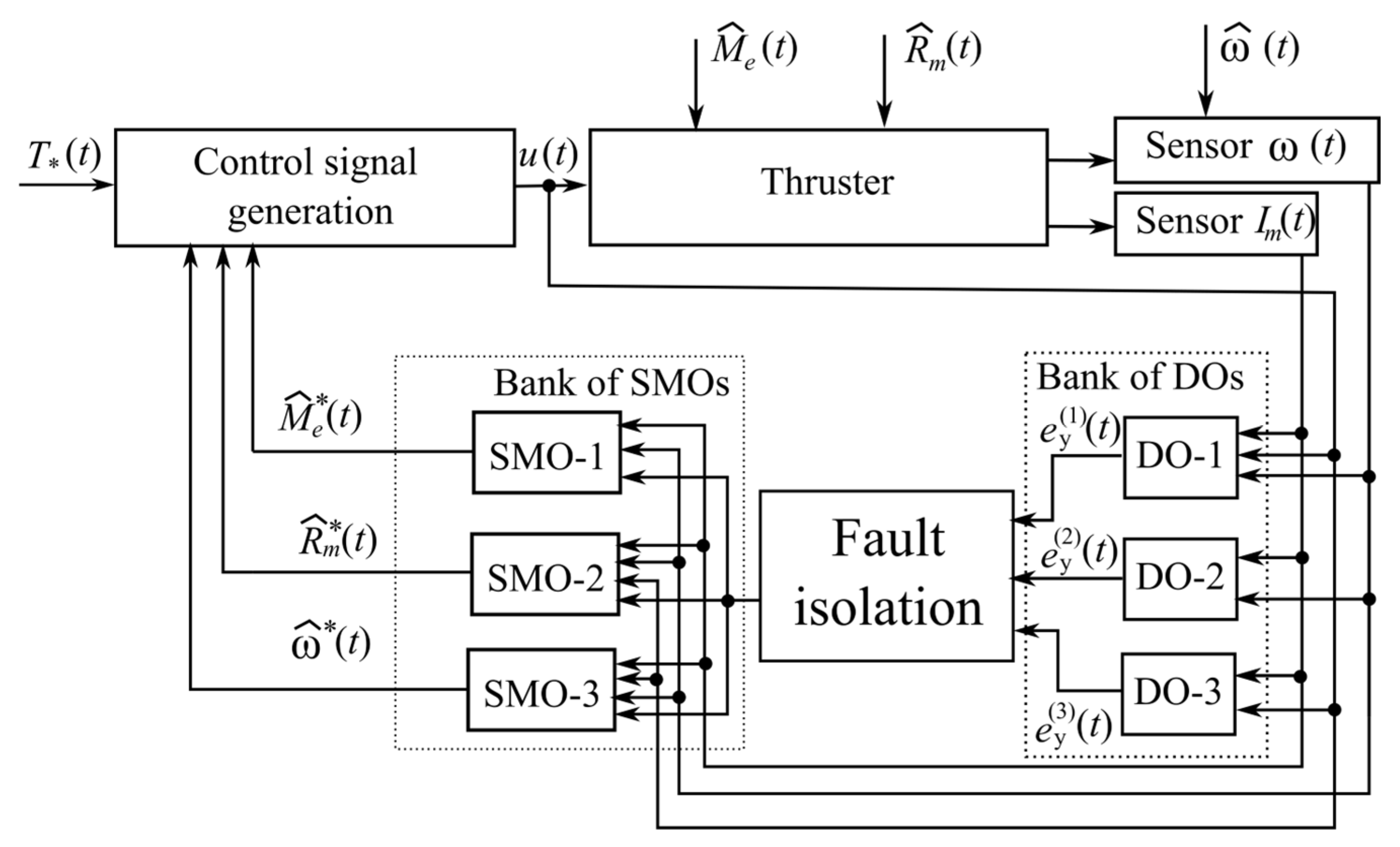
A schematic representation of the system for compensating for the consequences of single faults is depicted in Figure 2. Residual signals $e_y^{(1)}(t)$, $e_y^{\left(2\right)}\left(t\right)$, and $e_y^{(3)}(t)$ are generated by a bank of three DOs (23)–(25) and then the fault is isolated. Then, the values of ${\widehat{M}}_e^{*}(t)$, ${\widehat{R}}_m^{*}\left(t\right)$, or ${\widehat{\omega }}^{*}\left(t\right)$ are estimated by the corresponding SMO, (32), (33), or (34). Finally, these values are used for generating the control signals $u$ (46) for UR thrusters, as described by (1).

When the paired faults are detected and isolated, the appropriate compensating system shown in Figure 3 is used. Here, instead of SMO-3 (34), SMO-4 (35) and SMO-5 (36) are used. In addition, unlike Figure 2, the signals ${\omega }^4\left(t\right)$ and ${\omega }^5\left(t\right)$ are employed instead of the readings from the angular velocity sensor in DO-1 (23), DO-2 (24), SMO-1 (32), and SMO-2 (33).

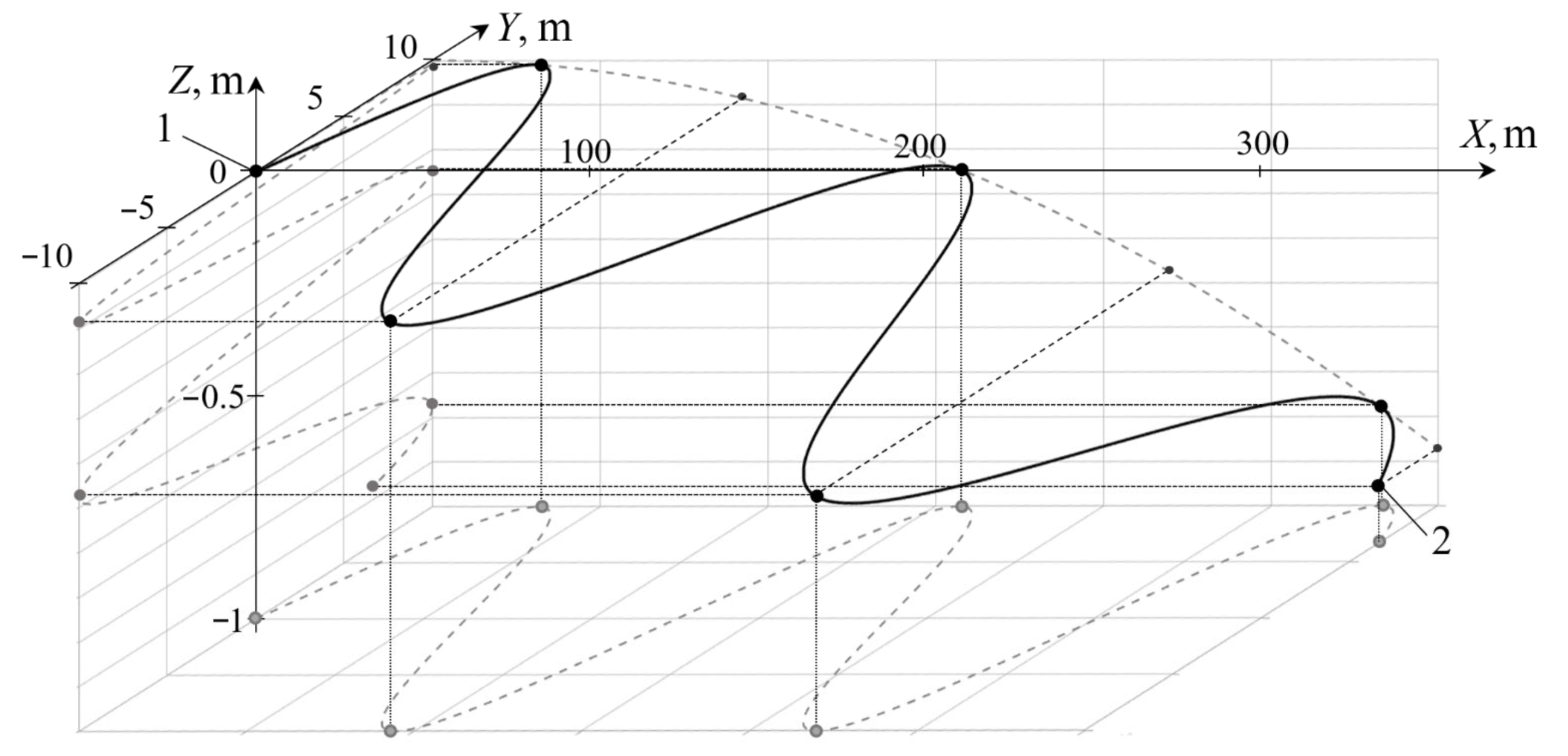
To check the effectiveness of the compensating system shown in Figure 2, computational simulating is carried out. For simulation, the UR with six thrusters (Figure 4) moving along the program trajectory $x(t)=t$ m, $y\left(t\right)=10sin\left(0.02t\right)$ m, $z\left(t\right)=5\cos \left(0.002t\right)-5$ m (see Figure 5) is considered. The beginning of the trajectory is indicated by the number 1 and the end by 2. Faults occur in the UR thruster creating the thrust $T_1$. The parameters of the UR are consistent with those outlined in [45].

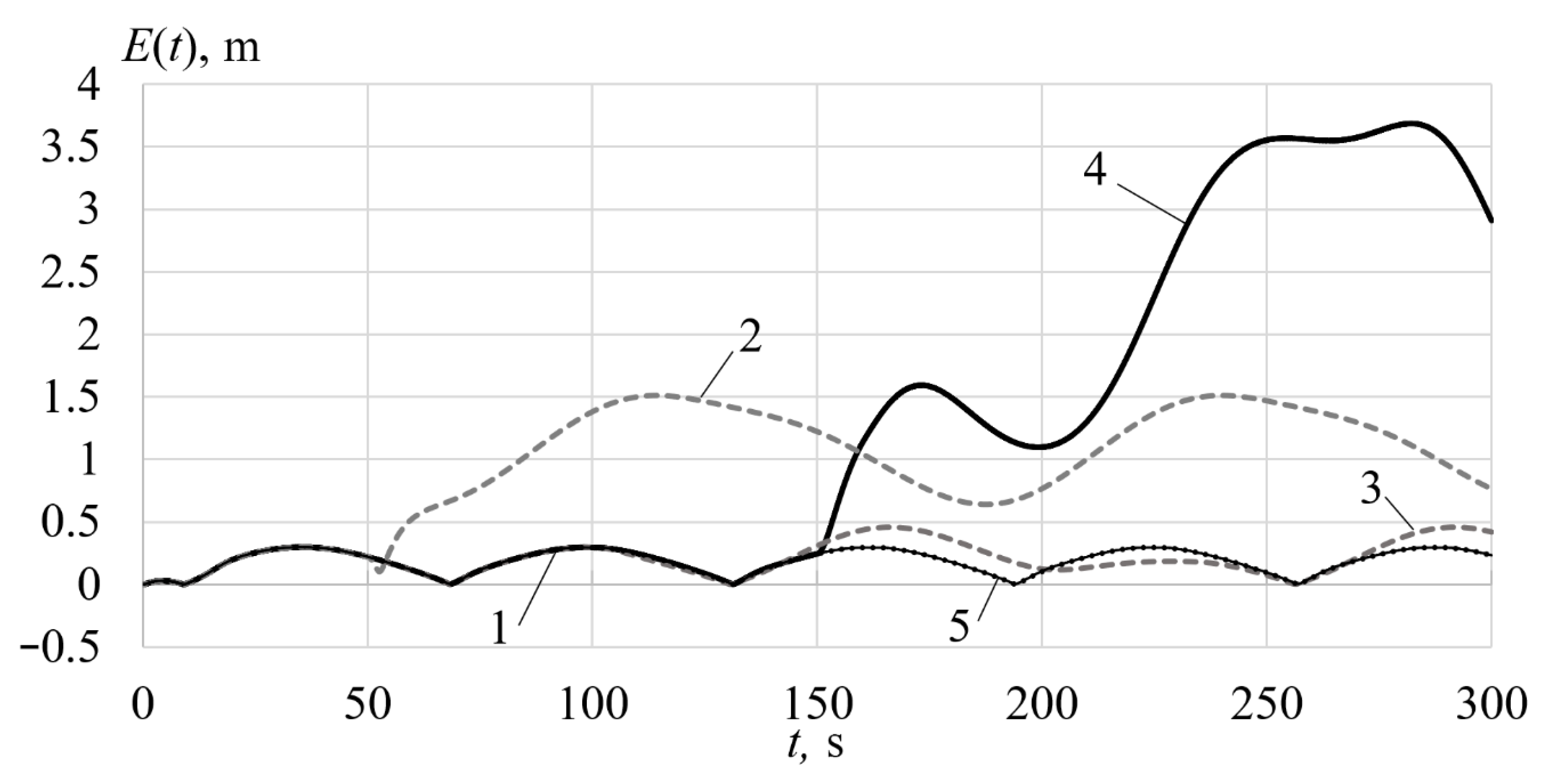
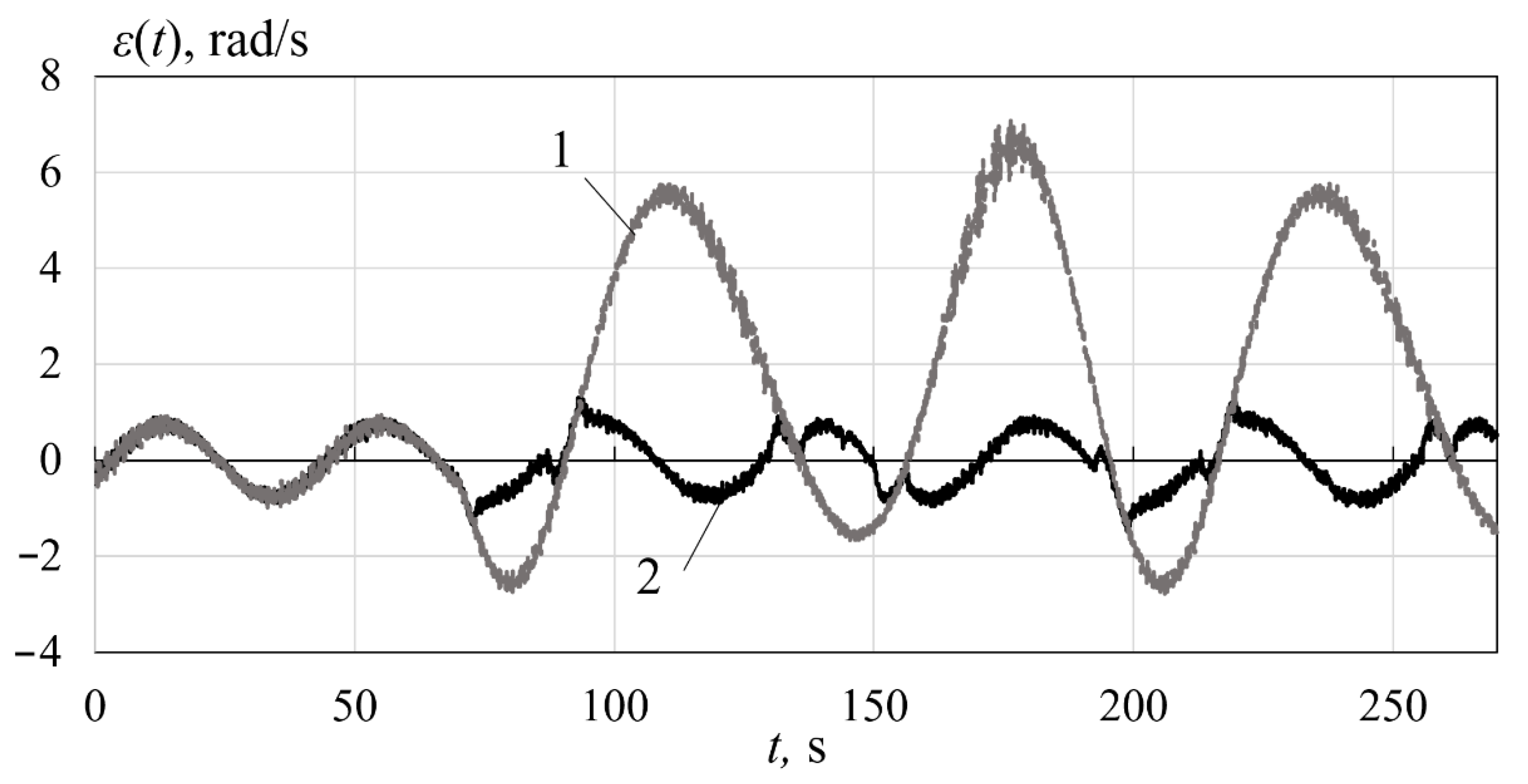
Simulation results in the form of the tracking errors of the UR with and without the compensating systems are shown in Figure 6. If there are no faults, the tracking error $E(t)$ of the UR does not exceed 0.3 m (see the curve 1 in Figure 6). But when the faults occur and the compensating system is not used, the accuracy of the UR movement decreases significantly.

Curve 2 in Figure 6 represents the graph of the tracking error when the error $\widehat{\omega }(t)=10$ rad/s occurs at $t=50$ s, which is about 30% of the average rotational speed of the propeller shaft. The tracking error grows to 1.51 m (in 5.03 times).

Curve 3 shows the tracking error where the active resistance of the propulsion armature increases by 30% (${\widehat{R}}_m(t)=0.6$ Ω) at $t=100$ s. The error increases to 0.46 m (by 53.3%).

Curve 4 indicates the error when an additional external torque ${\widehat{M}}_e(t)=0.5M_e(t)$ appears on the shaft of the specified thruster at $t=150$ s. This fault leads to an increase in the tracking error to 3.68 m (in 12.27 times).

Curve 5 shows the tracking error with any single faults where the proposed compensating system is used. In this case, the maximum deviation of the UR from the specified trajectory does not exceed 0.302 m. It should be added that the information about the non-zero function ${\widehat{R}}_m(t)$ can serve as an indicator for the overheating of the thruster and for a possible change in the mode (speed) of UR movement or for the complete termination of its mission.

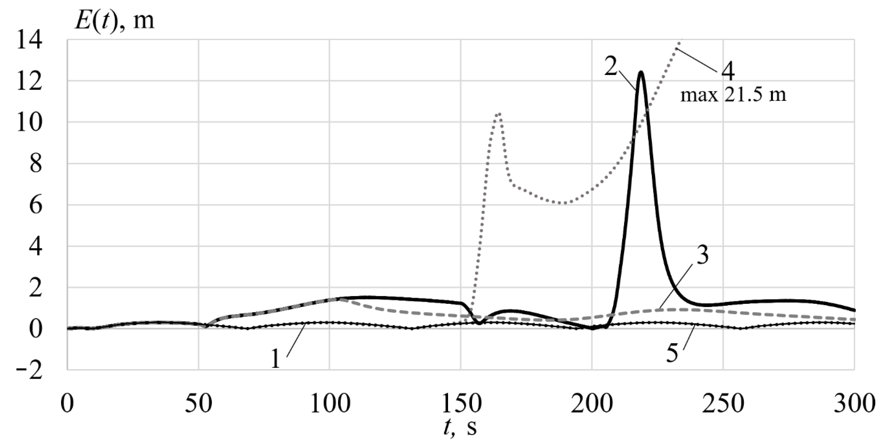
The results of computational simulation to verify the effectiveness of the system designed to compensate for the consequences of paired faults (see Figure 3) are shown in Figure 7. The magnitudes and time of appearance of faults are chosen to be the same as in the case with the single faults.

Curve 1 in Figure 7 shows the tracking error without any faults. Curve 2 shows the tracking errors when the errors ${\widehat{M}}_e(t)$ and $\widehat{\omega }(t)$ appear without compensating. In this situation, the tracking inaccuracy increases to 12.3 m (in 41.6 times). Curve 3 shows the graph of the tracking error when functions ${\widehat{R}}_m\left(t\right)$ and $\widehat{\omega }(t)$ appear. Here, the tracking error increases to 1.4 m (in 4.66 times). Curve 4 indicates the tracking error exceeds 21 m (in more than 70 times) when non-zero functions ${\widehat{M}}_e(t)$ and ${\widehat{R}}_m\left(t\right)$ appear. Curve 5 indicates the error when any combinations of the paired faults occur but the compensating system shown on Figure 3 is used. Obviously, this system stabilizes the tracking error at the nominal value for any set of the paired faults.

Thus, the simulation results show that the use of the compensating systems shown in Figure 2 and Figure 3 maintains the initial accuracy of the UR trajectory movement with the occurrence of single and paired faults. Similar results are obtained when the faults occur in the other thrusters of the UR.

3. Experimental Research

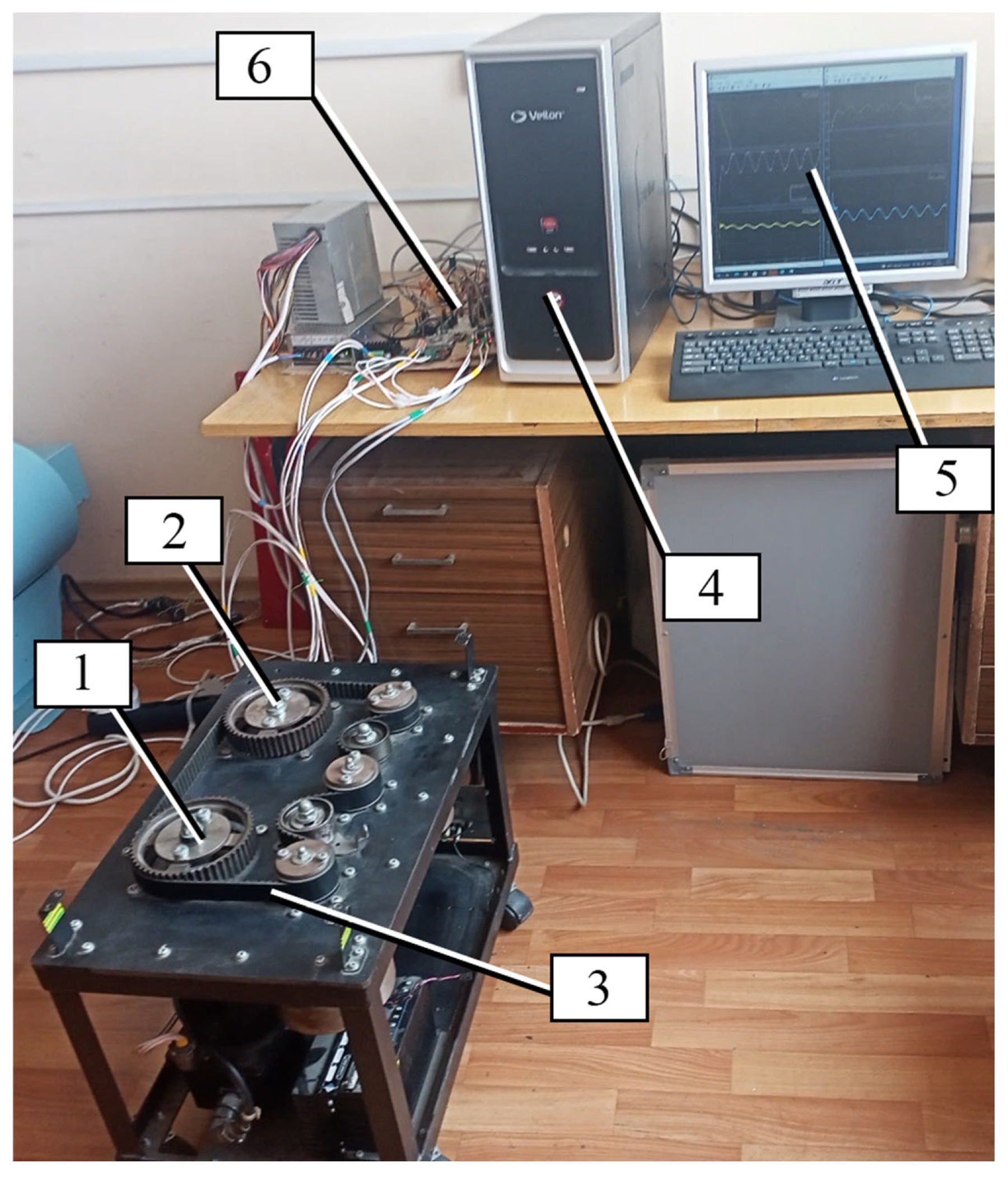
To verify the functionality of the proposed compensating system, in addition to computational simulation, a series of full-scale experiments were carried out using an electromechanical stand shown in Figure 8. It contains two DC electric motors with toothed pulleys on their output shafts (see Figure 8, numbers 1 and 2), connected by a belt drive (Figure 8, number 3). The sensors in the stand are a tachogenerator for measuring the speed of the rotation of the motor shafts and current sensors installed on both electric motors. A PC with Matlab 2021b software (Figure 8, number 4) was used to control the stand and display the appropriate information (Figure 8, number 5). The digital control of the stand was carried out using the ESP-32 microcontroller (Figure 8, number 6).

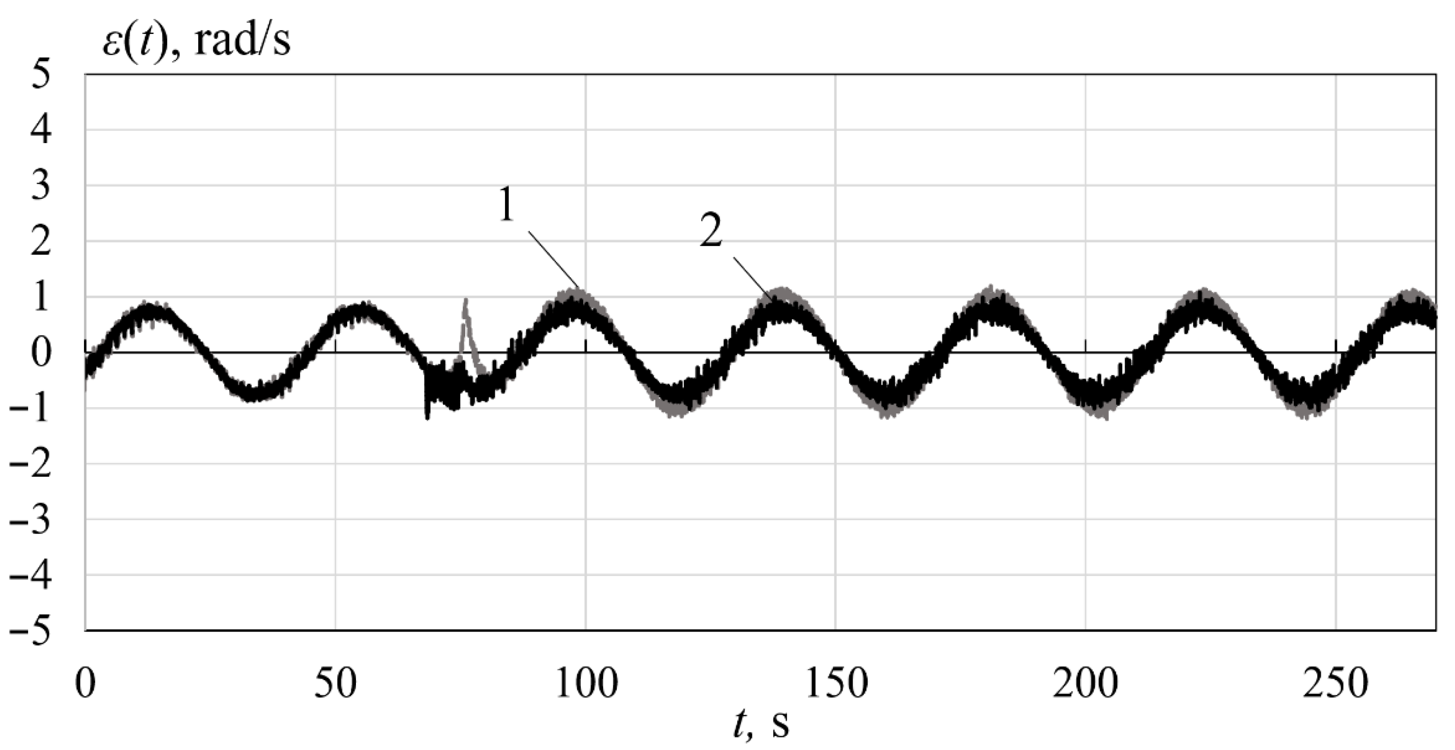
The appearance of an external load torque ${\widehat{M}}_e\left(t\right)$ is modeled by applying a constant $u_2=7$ V or alternating $u_2(t)=3.5\sin \left(0.4t\right)+3.5$ V voltage to the second electric drive of the stand preventing the rotation of the first electric motor. The appearance of the error $\widehat{\omega }\left(t\right)$ in the angular velocity sensor is modeled by software adding constant ($\widehat{\omega }=$5 rad/s) or variable ($\widehat{\omega }\left(t\right)=4\sin \left(0.1t\right)+2$ rad/s) signals to the real sensor readings.

During the experiment, the compensating system (see Figure 2 and Figure 3) ensures the rotation of the first electric motor with the angular velocity ${\omega }^{*}\left(t\right)=4\sin \left(0.15t\right)+16$ rad/s. It is assumed, for simplicity, that the error $\widehat{R}(t)=0$. This results in reducing the complex control law (51), and the simplified law compensating the influence of the load torque ${\widehat{M}}_e\left(t\right)$ is as follows:

$$u\left(t\right)=\tilde{U}\left(t\right)+{\displaystyle \frac{R_m}{k_u{k}_m}}{\widehat{M}}_e^{*}\left(t\right),$$

(47)

where $\tilde{U}\left(t\right)$ is the control signal generated by a standard PID controller.

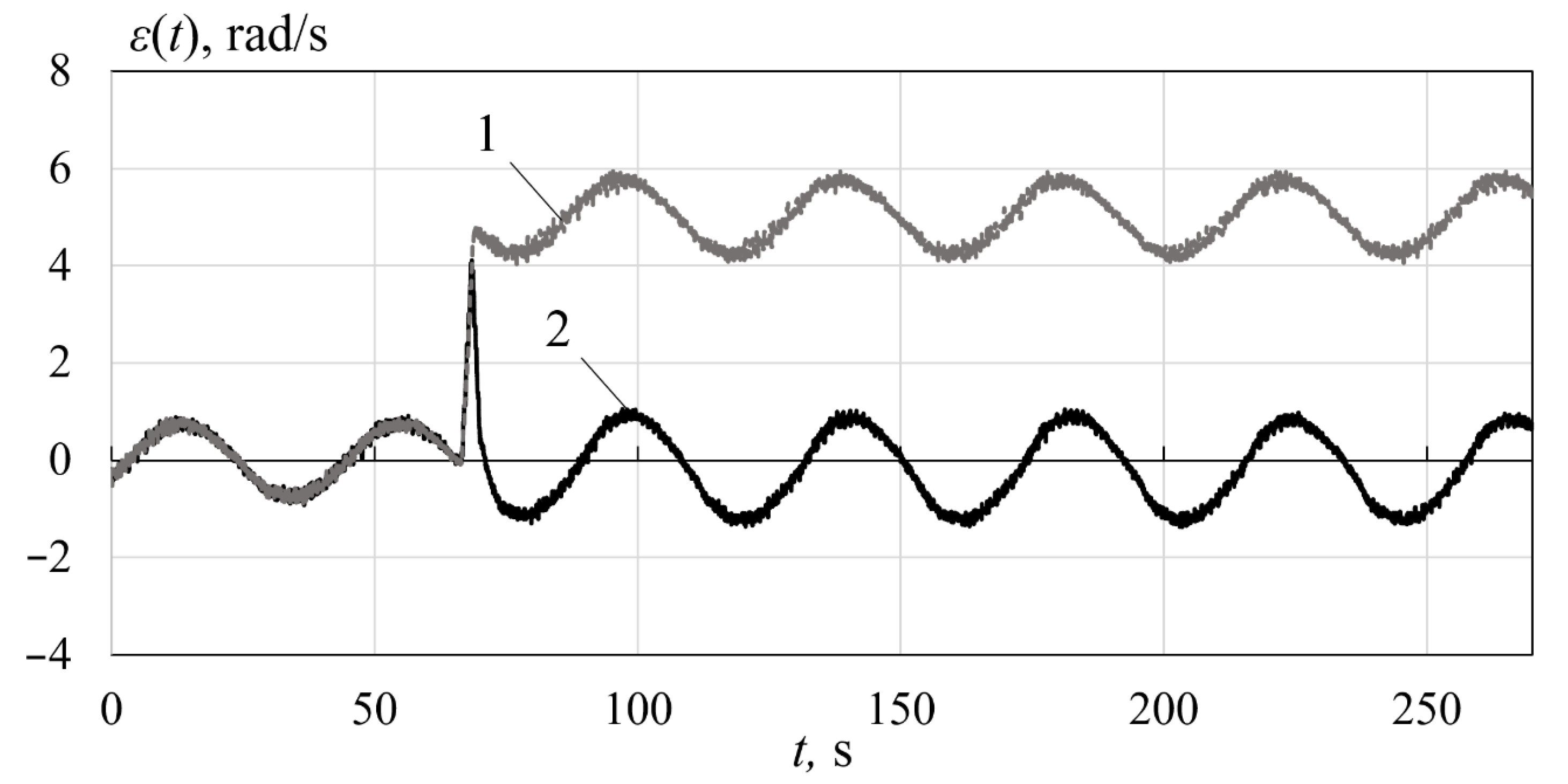
In Figure 9 and Figure 10, the errors $\epsilon (t)$ of the angular velocity of the electric motor when constant fault $\widehat{\omega }$ and variable $\widehat{\omega } \left(t\right)$ errors, respectively, occur at time $t=70$ s are shown. In these figures, curves 1 and 2 show the error $\epsilon (t)$ when only a standard PID controller and the compensating system are used, respectively.

As it follows from Figure 9, the appearance of the constant error $\widehat{\omega }$ increases the maximum errors $\epsilon (t)$ from 0.8 rad/s to 5.8 rad/s, i.e., 7.25 times. However, when the compensating system is used, the error $\epsilon (t)$ is only 1.1 rad/s, i.e., it is decreased 5.27 times.

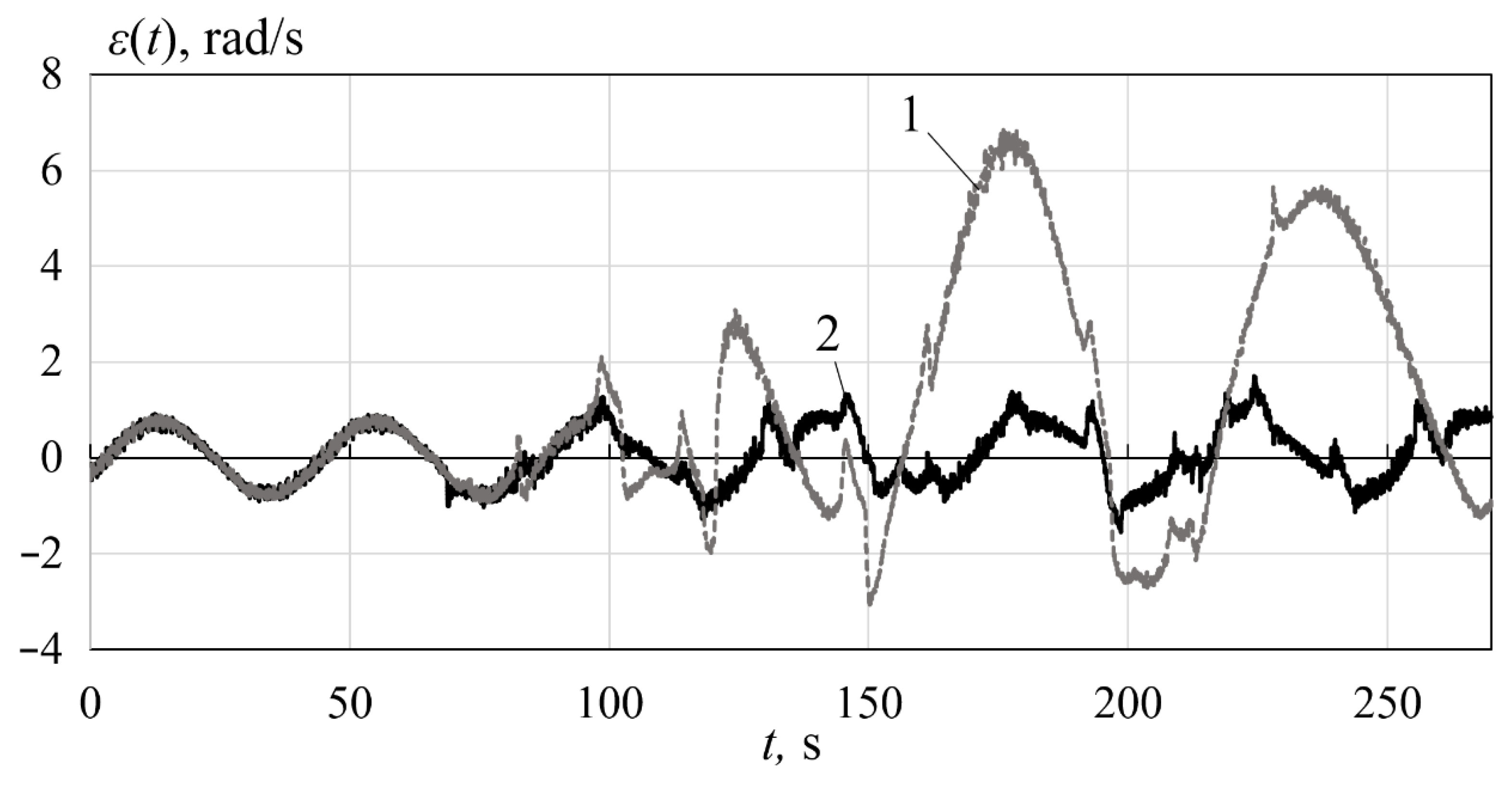
If a variable error $\widehat{\omega }(t)$ appears in the angular velocity sensor readings (see Figure 10), the maximum error $\epsilon (t)$ increases from 0.8 rad/s to 7.1 rad/s (8.87 times). The use of the compensating system reduces this error to 1.3 rad/s (6.82 times).

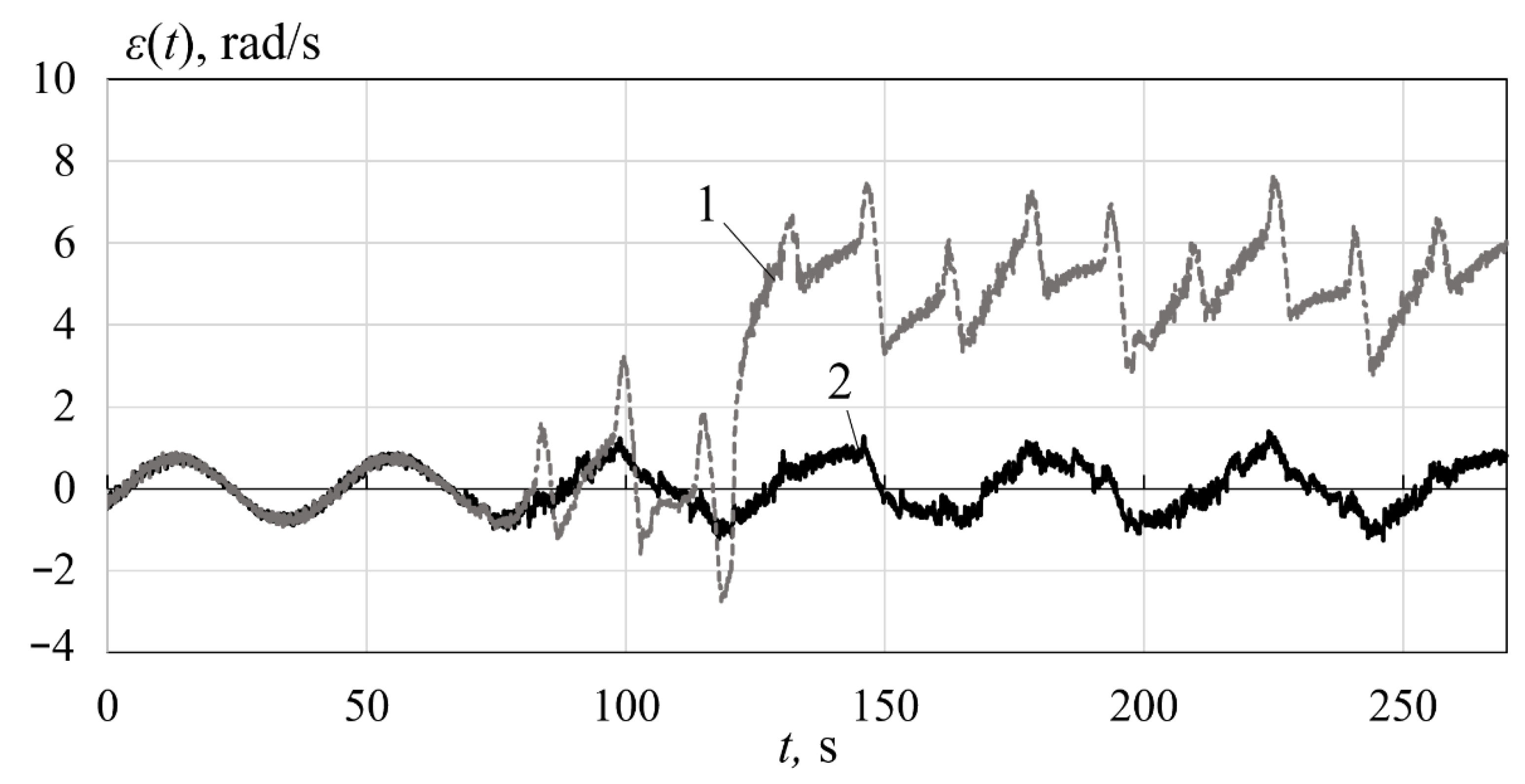
The errors of the angular velocity $\epsilon (t)$ of the first electric motor when the constant ${\widehat{M}}_e$ or variable ${\widehat{M}}_e\left(t\right)$ load torque is applied to its output shaft are shown in Figure 11 and Figure 12, respectively. One can see from these figures that under the constant load the maximum error $\epsilon (t)$ increases to 1.1 rad/s (by 37.5%) and under the variable load it increases to 3.2 rad/s (4 times). When the compensating system is used, the maximum errors $\epsilon (t)$ are 1 rad/s and 1.3 rad/s for the constant and variable load torque, respectively. Thus, the use of the compensating system reduces the errors $\epsilon (t)$ by 9% in the first case and 2.4 times in the second.

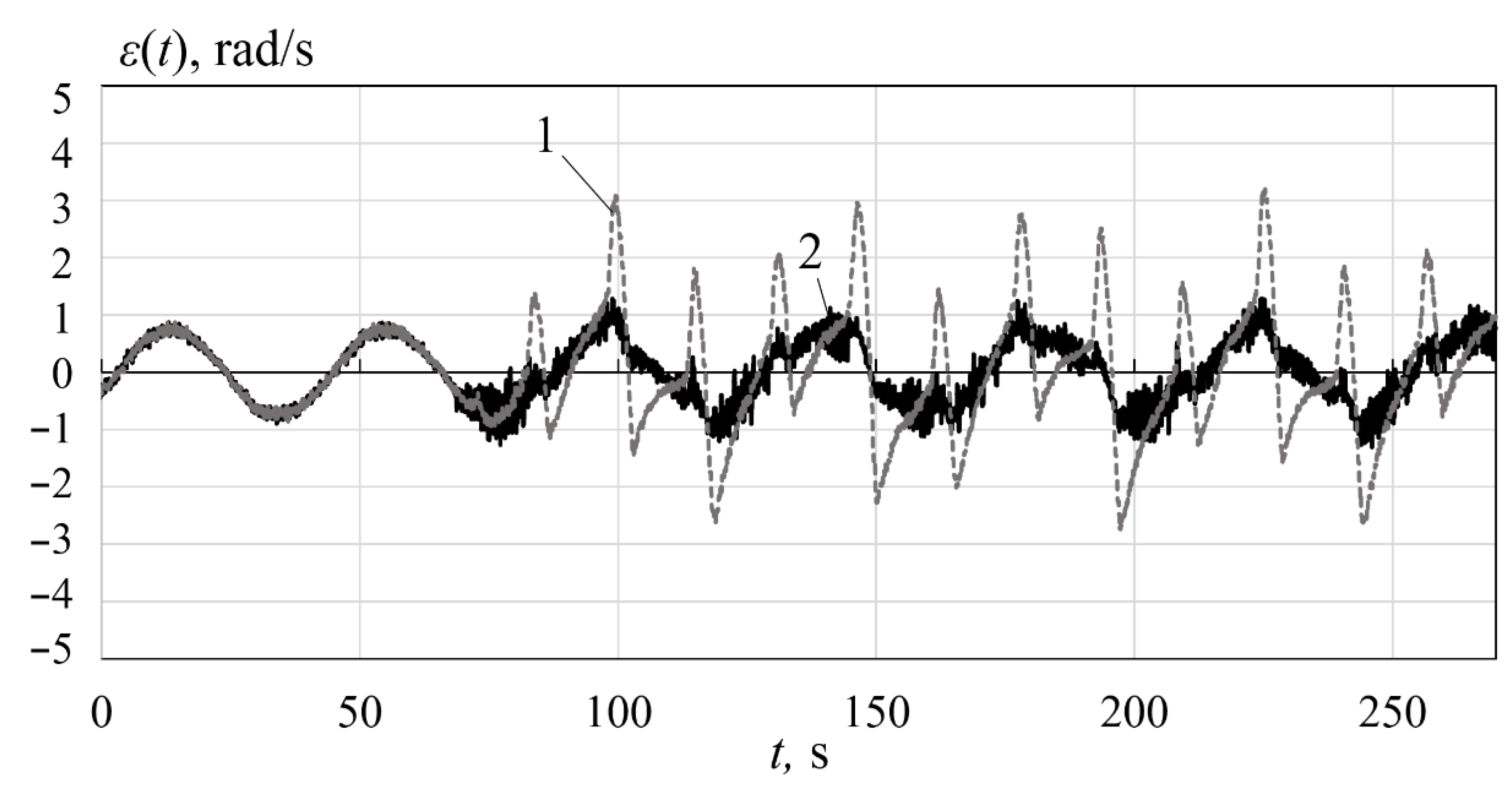
In Figure 13 and Figure 14, the error $\epsilon (t)$ under the paired fault is shown. Figure 13 shows the graph of this error when the variable load moment ${\widehat{M}}_e\left(t\right)$ and the constant error $\widehat{\omega }$ occur at $t=70$ and $t=120$, respectively. On the other hand, in Figure 14, the variable error $\widehat{\omega }(t)$ is used. From these figures it is clear that the indicated paired fault leads to an increase in the maximum error $\epsilon (t)$ to 7.5 rad/s (9.37 times) in the first case and to 6.9 rad/s (8.62 times) in the second. The compensating system shown in Figure 3 reduces this error to 1.6 rad/s (4.68 times) and to 1.7 rad/s (4.05 times), respectively.

Thus, the results of full-scale experiments fully confirm the high efficiency of the suggested compensating system when various single and paired faults occur.

4. Conclusions

This article has developed a method of designing the systems for detecting, estimating, and compensating for the consequences of faults. These systems provide an accurate estimation of the values of single and paired changes for all parameters in the UR thrusters from their nominal values and inaccuracies in the readings of their angular velocity sensors. Based on the well-known method of nonlinear controller design, these systems have been developed to compensate for the effects of single and paired faults. These systems enable the continued functioning and stabilization of the critical parameters of these propulsion systems in the event of unforeseen faults. The performance and operability of the proposed system was verified through computational simulation and full-scale experiments using the electromechanical stand.